Time variations of rainfall erosivity factor in the Czech Republic

In the first half of the 20th _{century in the USA,}

a need emerged for the calculation of the soil loss caused by water erosion. For this purpose Cook (1936) identified 3 main factors determining the processes of water erosion: susceptibility (soil erodibility), the potential erosivity of rainfall and runoff, and the soil protection afforded by plant cover. Zingg (1940) published the first empirical model of the erosion process for evaluating average annual losses of soil due to water erosion which he derived from the results of an extensive research into the influence of the steepness and length of a slope on this process. The initial research into the forecasting methods for calculating soil loss due to erosion has been carried out in USA by the following authors: Smith (1941), Musgrave (1947), Browning et al. (1948), Smith and Whitt (1948), and others.

Until today, the best description of the quantita-tive influence of the main factors of water erosion caused by storm rainfall (USLE) was given by Wisch- meier (1959). The Universal Soil Loss Equation

(USLE) describes the soil loss caused by water (G) as a product of six factors: rainfall-runoff erosiv-ity (R), soil erodibilerosiv-ity (K), slope length (L), slope steepness (S), cover and management practices (C), and supporting conservation practices (P).

G = R × K × L × S × C × P

This relatively simple method enables the cal-culation of the hypothetical long term average annual soil loss caused by water erosion in any given area. It has the advantage of being easily available and simple in the access.

Since its publication in the Agriculture Hand-book No. 282 (Wichmeier & Smith 1965) and its revised version published in the Agriculture Handbook No. 537 (Wichmeier & Smith 1978) USLE has become the main planning instrument for the soil protection in the USA and around the world.

By integrating new findings, experiences and a large amount of digitally processed data acquired

Supported by the Ministry of Agriculture of the Czech Republic, Project No. QH72085

Time Variations of Rainfall Erosivity Factor

in the Czech Republic

Eliška KUBÁTOVÁ, Miloslav JANEČEK and Dominika KOBZOVÁ

Department of Land Use and Improvement, Faculty of Environmental Sciences, Czech University of Life Sciences in Prague, Prague, Czech Republic

Abstract: The ombrographic data have been selected from 24 meteorological stations of the Czech Hydro Meteoro-logical Institute (CHMI), according to the terms of the Universal Soil Loss Equation for calculating the long term loss of soil through water erosion, erosion hazard rains and their occurrence, with their relative amounts and erosiveness, R-factors determined for each month. By comparing the value of the time division of the R-factor in the area of the Czech Republic and in the selected areas of the USA, it has been demonstrated that this division may be applied in the conditions of the Czech Republic.

since 1978, which manifested itself also by changes in the calculations of each factor, the so called RUSLE “Revised Universal Soil Loss Equation“ was created by Renard et al. (1997) and Toy et al. (1999), and which uses the same algorithm as USLE.

Aims

The purpose of this study is to compare the occurrence of erosion rainfall, characterised by the R-factor values of each month in the Czech Republic, with the data acquired from the selected meteorological stations in the USA, and to dem-onstrate the validity of the calculation procedure

of the R-factor according to USLE also in our country. The issue has also been dealt with in other European countries, i.e. by Schwertmann

et al. (1987), Boardman and Poesen (2006), in Bavaria, Austria and Belgium.

The rainfall factor – R, i.e. its erosivity, was formulated in the USA (Wischmeier & Smith 1965). The aforementioned had the largest amount of the necessary data accessible at that time, ac-quired from a network of meteorological survey stations situated throughout the USA. The rainfall factor used for determining the average annual loss of soil includes the influence of exceptional precipitation events (intensive rainfall) as well as average intensive rains.

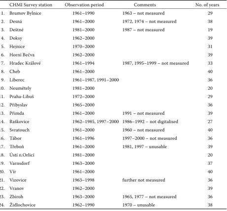
Table 1. List of CHMI ombrographic survey stations used in the calculation of the R-factors

CHMI Survey station Observation period Comments No. of years

1. Brumov Bylnice 1961–1990 1963 – not measured 29

2. Desná 1961–2000 1972, 1974 – not measured 38

3. Deštné 1981–2000 1987 – not measured 19

4. Doksy 1962–2000 39

5. Hejnice 1970–2000 31

6. Horní Bečva 1962–2000 39

7. Hradec Králové 1961–1994 1987, 1995–1999 – not measured 33

8. Cheb 1961–2000 40

9. Liberec 1961–1987, 1991–2000 36

10. Neumětely 1981–2000 20

11. Praha-Libuš 1972–2000 29

12. Přibyslav 1965–2000 36

13. Přimda 1961–2000 1991 – not measured 39

14. Raškovice 1962–1985, 1997–2000 1986–1992 – not digitalised 27

15. Svratouch 1961–2000 1960 – not measured 40

16. Tábor 1961–1996 1997–2000 – not measured 36

17. Třeboň 1961–2000 1981, 1997 – unusable 39

18. Ústí n.Orlicí 1981–2000 20

19. Varnsdorf 1963–2000 37

20. Vír 1961–2000 40

21. Vizovice 1963–1998 further not measured 36

22. Vranov 1962–2000 39

23. Zbiroh 1963–2000 1965, 1977 – not measured 36

The data indicate that, when the factors other then rainfall are held constant, the soil losses in an area are directly proportional to the rainstorm parameter: total storm energy (E) times the maxi-mum 30-min intensity (i₃₀):

R = E × i₃₀/100 where:

R – rainfall erosivity factor (MJ/ha × cm/h) E – total storm energy (cm/h)

i₃₀ – maximum 30-min intensity (cm/h)

The total storm energy is: _n

E = ∑ E_i

i=1

where:

E_i – kinetic energy of rain in the i-section (n – number

of rain sections):

E_i = (206 + 87 log i_si) × H_si

where:

i_si – intensity of rain in the i-section (cm/h)

H_si – rain fall in the i-section (cm)

The annual value of the R-factor is determined from long term data records of precipitations and represents the aggregate of the erosion impact of

each storm rainfall occurring in the given year. Rain showers of less then 12.5 mm (0.5 inch) were omit-ted from the erosion index, unless at least 6.25 mm (0.25 inch) of rain fell in 15 min. The delay between the rainfalls must be longer then 6 hours in order to consider them as individual rainfalls.

Therefore, the rainfall erosivity factor R depends on the frequency of occurrence, kinetic energy, intensity and amount of rain which fell. In the USA, the values of the R-factor were statistically assessed and presented in the form of an isoero-dent maps.

METhodoLoGY

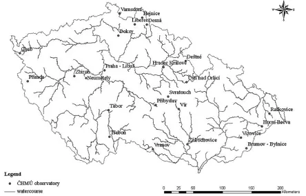
During the calculation of the R-factor for the region of the Czech Republic, the ombrographic data were available, collected from 24 selected sur-vey stations of the CHMI; the method of Wisch- meier and Smith (1978) was systematically im-plemented. Preference was given to the survey stations producing long term ombrographic servation data (Table 1 and Figure 1). The ob-servations were carried out only in the growing season, since most ombrographs are not equipped with heating.

The data records were fed into a text editor in the digital form at time intervals of 1 min, and were adapted from the text document to the Excel chart processor, where R-factor values were sub-sequently calculated. Prior to that, the calculated data were screened (screening out the precipita-tion events which did not comply with the above mentioned criteria) and adapted from the text to the Excel chart processor, where R-factor values were subsequently calculated.

RESULTS

Calculations of the R-factors were carried out in 2 variants:

V1. variant – comprised rains which met 1 of the 2 requirements, i.e. when the rainfall was more than 12.5 mm, or when 6 mm fell within a period of 15 min.

V2. variant – comprised rains meeting both require-ments, i.e. the rainfall above 12.5 mm and with an intensity above 6 mm in 15 min.

The following data were determined by the survey stations, as indicated in Table 1 and Figure 1: (a) – relative number of erosion rains which

oc-curred each month, including their aggregate expression,

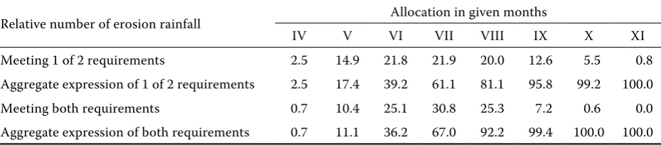
(b) – R-factors value expressed in the percentage of occurrence in each month and on aggregate. The number of occurrences of erosion rainfall and their long term variations during the given Table 2. Average number of erosion hazard precipitations in the given months

Relative number of erosion rainfall Allocation in given months

IV V VI VII VIII IX X XI

Meeting 1 of 2 requirements 2.5 14.9 21.8 21.9 20.0 12.6 5.5 0.8

Aggregate expression of 1 of 2 requirements 2.5 17.4 39.2 61.1 81.1 95.8 99.2 100.0

Meeting both requirements 0.7 10.4 25.1 30.8 25.3 7.2 0.6 0.0

Aggregate expression of both requirements 0.7 11.1 36.2 67.0 92.2 99.4 100.0 100.0

0 10 20 30 40 50 60 70 80 90 100

IV V VI VII VIII IX X XI

Month

(%

)

Relative number of ranifall for 1 of 2 requirements

Relative number of rainfall for 1 of 2 requirements - mass curve Relative number of rainfall for both requirements

Relative number of rainfall for both requirements - mass curve

Figure 2. Record of the average occur-rence of erosion rainfall during the year

–

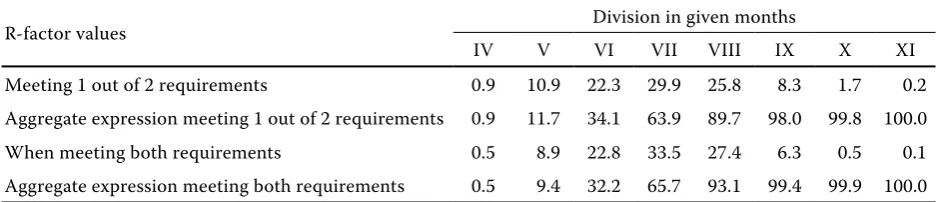
Table 3. R-factor values in the given months

R-factor values Division in given months

IV V VI VII VIII IX X XI

Meeting 1 out of 2 requirements 0.9 10.9 22.3 29.9 25.8 8.3 1.7 0.2

Aggregate expression meeting 1 out of 2 requirements 0.9 11.7 34.1 63.9 89.7 98.0 99.8 100.0

When meeting both requirements 0.5 8.9 22.8 33.5 27.4 6.3 0.5 0.1

Aggregate expression meeting both requirements 0.5 9.4 32.2 65.7 93.1 99.4 99.9 100.0

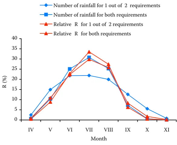
Table 4. Comparing the number of erosion rainfall with R-factor values

Division in given months

IV V VI VII VIII IX X XI

Number of rainfall for 1 out 2 requirements 2.5 14.9 21.8 21.9 20.0 12.6 5.5 0.8

Relative R for out of 2 requirements 0.7 10.4 25.1 30.8 25.3 7.2 0.6 0.0

Number of rainfall for both requirements 0.9 10.9 22.3 29.9 25.8 8.3 1.7 0.2

Relative R for both requirements 0.5 8.9 22.8 33.5 27.4 6.3 0.5 0.1

Figure 3. Evolution of R-factor average divisions during one year

months were determined from the processed data – see Table 2 and Figure 2.

On the basis of the observed variations in the ero-sion rainfall during each month, it was confirmed that their highest occurrence took place during the summer months (June–August), see Tables 3, 4, 5 and Figures 3, 4, 5. Significantly increased and decreased numbers of erosion rainfalls occurred

during the indicated months in the form of rains meeting both requirements. A similar change was determined in the R-factor division while the difference between both groups was not very significant (up to 2%).

Comparing the respective values of the R-factor division over a year in each month surveyed, as recommended for the practical use in the regions 0

10 20 30 40 50 60 70 80 90 100

IV V VI VII VIII IX X XI

Month

(%

)

Relative "R" for 1 of 2 requirements

Relative "R" for 1 of 2 requirements - mass curve Relative "R" both requirements

Relative "R" both requirements - mass curve

–

–

0 5 10 15 20 25 30 35 40

IV V VI VII VIII IX X XI

Month

(%

)

Number of rainfall for 1 out of 2 requirements Number of rainfall for both requirements Relative "R" for 1 out of 2 requirements Relative "R" for both requirements

0 10 20 30 40 50 60 70 80 90 100

IV V VI VII VIII IX X XI

Month

(%

)

Relative number of rainfall for 1 out of 2 requirements - mass curve Relative number of rainfall for both requirements - mass curve Relative "R" for 1 out of 2 requirements - mass curve

Relative "R" for both requirements - mass curve

Table 5. Aggregate expression of the number of rainfall with R-factor values

Division in given months

IV V VI VII VIII IX X XI

Relative number of rainfall for 1 out of 2 requirements 2.5 17.4 39.2 61.1 81.1 95.8 99.2 100

Relative number of rainfall for both requirements 0.7 11.1 36.2 67.0 92.2 99.4 100.0 100

Relative R for 1 out of 2 requirements 0.9 11.7 34.1 63.9 89.7 98.0 99.8 100

Relative R for both requirements 0.5 9.4 32.2 65.7 93.1 99.4 99.9 100

Figure 4. Evolution of the number of erosion rainfall and R-factor values

Figure 5. Total curves of number of erosion rainfall with R-factor values –

R

–

R

0 5 10 15 20 25 30 35 40

IV V VI VII VIII IX X XI

Month

(%

R

)

N Montana NE Montana

S Montana SE Montana

NE Wyoming N a S Dakota, Minnesota

Average

0 10 20 30 40 50 60 70 80 90 100

IV V VI VII VIII IX X XI

Month

(%

)

N Montana NE Montana

S Montana SE Montana

NE Wyoming N a S Dakota, Minnesota

Average

Figure 6. Annual variations of the R-factor in the North West regions of the USA

Figure 7. Total curves of the relative values of R-factors for the selected regions in the North West of the USA

R

(

%

)

R

(

%

Table 6. Monthly division of the R-factors for 6 meteorological survey stations in the North West of the USA

Survey station Percentage division of the R-factor

IV V VI VII VIII IX X XI

N Montana 0.9 16.4 35.9 22.7 17.8 5.3 1.0 0

NE Montana 0.4 9.1 33.2 28.4 20.8 7.1 1.0 0

S Montana 2.6 17.0 29.3 24.6 16.0 8.8 1.7 0

SE Montana 1.6 15.4 35.5 23.1 15.6 7.5 1.2 0

NE Wyoming 2.5 15.0 28.6 26.6 20.1 5.6 1.6 0

N a S Dakota, Minnesota 2.0 8.0 25.0 27.0 27.0 8.0 2.0 0

Average 1.7 13.5 31.3 25.4 19.6 7.1 1.4 0

Table 7. Total curves of the R-factor division for 6 meteorological survey stations in the North West of the USA

Survey station Percentage division of the R-factor

IV V VI VII VIII IX X XI

N Montana 0.9 17.3 53.2 75.9 93.7 99.0 100.0 100.0

NE Montana 0.4 9.5 42.7 71.1 91.9 99.0 100.0 100.0

S Montana 2.6 19.6 48.9 73.5 89.5 98.3 100.0 100.0

SE Montana 1.6 17.0 52.5 75.7 91.3 98.8 100.0 100.0

NE Wyoming 2.5 17.5 46.1 72.7 92.8 98.4 100.0 100.0

N a S Dakota, Minnesota 3.0 11.0 36.0 63.0 90.0 98.0 100.0 100.0

Average 1.8 15.3 46.6 72.0 91.5 98.6 100.0 100.0

Figure 8. Evolution of the average monthly division of the R-factor in the North and the North West of the USA

0 20 40 60 80 100

IV V VI VII VIII IX X XI

Month

(%

)

Relative value of the "R" factor - mass curve

Division of "R" faktor in the months of vegetation period

R

0 20 40 60 80 100

IV V VI VII VIII IX X XI

Month

R

(%)

Relativ value of the "R" faktor - mass curve

Division of "R" faktor in months of vegetation period

0 20 40 60 80 100

IV V VI VII VIII IX X XI

Month

R

(%

)

Relative value of the R - Factor - mass curve

Division of R - Factor in the months of vegetation period

Table 9. Comparative values of R-factor division for the Czech Republic, the USA and Bavaria

Factor values Division in given months

IV V VI VII VIII IX X XI

R division for the Czech Republic 0.9 10.9 22.3 29.9 25.8 8.3 1.7 0.2

R division for the USA 1.7 13.5 31.3 25.4 19.6 7.1 1.4 0.0

R division for Bavaria 3 10.3 28.0 20.9 20.6 9.8 3.2 1.6

Figure 9. Evolution of the R-factor di-vision during the vegetation period months for the North East of Mon-tana

Figure 10. Evolution of the average R-factor division during the given months in Bavaria

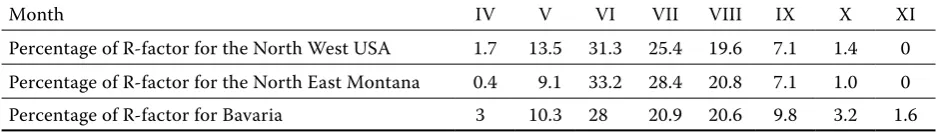
Table 8. Average division of the R-factor in given months for the North and the North West of the USA, North East part of Montana and Bavaria

Month IV V VI VII VIII IX X XI

Percentage of R-factor for the North West USA 1.7 13.5 31.3 25.4 19.6 7.1 1.4 0

Percentage of R-factor for the North East Montana 0.4 9.1 33.2 28.4 20.8 7.1 1.0 0

Percentage of R-factor for Bavaria 3 10.3 28 20.9 20.6 9.8 3.2 1.6

–

– R-f

of Bohemia and Moravia in previous publications by Janeček et al. (2005, 2007), no significant vari-ation has been found.

diSCUSSion

For the purpose of comparing the results of the average division of R-factors in the given months in the Czech Republic, we used the mass curve of average annual E_i parameter values from 140 meteorological survey stations situated in the USA (Renard et al. 1997).

Out of these stations, 6 had been selected with regard to climatic conditions similar to those in the Czech Republic. These stations are situated in the North and North West of the USA (Montana, North and South Dakota, Wyoming and Minne-sota). For these selected stations, the percentage division of the R-factor in the given months is shown in Table 6 and Figure 6, and the relative R-factors expressed by mass curves are shown in Table 7 and Figure 7. From the data supplied the average percentage division of the R-factor in the North and North West has been calculated – see Table 8 and Figure 8.

0 10 20 30 40 50 60 70 80 90 100

IV V VI VII VIII IX X XI

Month

(%

R

)

Relative "R" - mass curve, (CZ)

"R" divisions in vegetation months, (CZ) Relative "R" - mass curve, (USA)

"R" divisions in vegetation months, (USA) Relative "R" - mass curve, (Bavaria)

"R" divisions in vegetation months, (Bavaria)

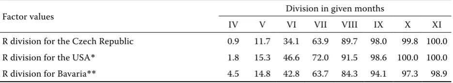
Table 10. Comparing long term evolution of monthly values of R-factors in the Czech Republic, the USA and Ba-varia

Factor values Division in given months

IV V VI VII VIII IX X XI

R division for the Czech Republic 0.9 11.7 34.1 63.9 89.7 98.0 99.8 100.0

R division for the USA* 1.8 15.3 46.6 72.0 91.5 98.6 100.0 100.0

R division for Bavaria** 4.5 14.8 42.8 63.7 84.3 94.1 97.3 98.9

*Division of R-factor begins with third month; **division of R-factor covers whole year

Figure 11. Long term evolution of the average R-factor by months in the Czech Republic, the USA, and Bavaria

R–

R–

R–

R

(

%

To specify further, the data from the survey stations in the North East parts of Montana have been processed showing the greatest similarities with the R-factor values measured in the Czech Republic – see Table 8 and Figure 9. Furthermore, the data from18 meteorological survey stations from neighbouring Bavaria were used for com-parison (Schwertmann et al. 1987) – see Table 8 and Figure 10. The overall comparison of these values for Montana, Bavaria, and our country is indicated in Tables 9 and 10, and in Figure 11.

ConCLUSion

The comparison of long term monthly occur-rences of erosion rainfall characterised by the divisions of R-factor values for the Czech Republic and selected survey stations in the USA indicates the occurrence of erosion rainfall in our conditions at the end of spring and the beginning of sum-mer (VII–VIII). The results indicated conformity of their division in the Czech Republic and the selected regions of the USA. Therefore, it may be considered that the use of the R-factor in the USLE complies with our conditions.

References

Boardman J., Poesen J. et al. (2006): Soil Erosion in Europe. John Wiley & Sons, Ltd., Chichester.

Brovning F.M., Norton R.A., McCall A.G., Bell F.G. (1948): Investigation in erosion control and the reclamation of land at the Missouri Valley Loess Con-servation Experiment Station, Clarinda, Iowa, 1931 – 42, U.S. Dep. Agric. Tech. Bull. 959.

Cook H.L. (1936): The nature and controlling variables of the water erosion process. Soil Science Society of America, 1: 60–64.

Janeček M. et al. (2005): Protection of Agricultural Soils from the Soil Erosion. ISV Praha. (in Czech)

Janeček M. et al. (2007): Protection of Agricultural

Soils from the Soil Erosion. Methodology. VÚMOP, Praha. (in Czech)

Musgrave G.W. (1947): The quantitative evaluation of factors in water erosion: A first approximation. Journal of Soil and Water Conservation, 2: 133–138.

Renard K.G., Foster G.R., Weesies G.A., McCool D.K., Yoder D.C. (1997): Predicting soil erosion by water: A guide to conservation planning with the Revised universal soil loss equation (RUSLE). USDA Agriculture Handbook No. 703, United States Depart-ment of Agriculture (USDA), Agricultural Research Service, Washington.

Schwertmann U., Vogel W., Kainz M. et al. (1987): Bodenerosion durch Wasser. Vorhersage des Abtrags und Bewertung von Gegenmassnahmen. E. Ulmer GmbH and Co., Stuttgart.

Smith D.D. (1941): Interpretation of soil conserva-tion data for field use. Agricultural Engineering, 22: 173–175.

Smith D.D., Whitt D.M. (1948): Evaluating soil loss-es from field areas. Agricultural Engineering, 29: 394–398

Toy T.J., Foster G.R., Renard K.G. (1999): RUSLE for mining, construction, and reclamation land. Journal of Soil and Water Conservation, 54: 462–467

Wischmeier W.H. (1959): A rainfall erosion index for a universal soil – loss equation. Soil Science Society of America Proceedings, 23: 246–248.

Wischmeier W.H., Smith D.D. (1965): Predicting rain-fall erosion losses from cropland east of the Rocky Mountains. Agricultural Handbook No. 282, United States Department of Agriculture (USDA), Agricul-tural Research Service, Washington.

Wischmeier W.H., Smith D.D. (1978): Predicting Rain-fall Erosion Losses – A Guide to Conservation Plan-ning. USDA Agriculture Handbook No. 537, United States Department of Agriculture (USDA), Agricul-tural Research Service, Washington.

Zingg A.W. (1940): Degree and length of land slope as it affects soil loss in runoff. Agricultural Engineering, 21: 59–64.

Received for publication February 23, 2009 Accepted after corrections July 2, 2009

Corresponding author:

Prof. Ing. Miloslav Janeček, DrSc., Česká zemědělská univerzita v Praze, Fakulta životního prostředí, katedra biotechnických úprav krajiny, Kamýcká 129, 165 21, Praha 6-Suchdol, Česká republika