Virtual Examples for Text Classification with Support Vector Machines
Manabu Sassano Fujitsu Laboratories Ltd. 4-1-1, Kamikodanaka, Nakahara-ku,
Kawasaki 211-8588, Japan [email protected]
Abstract
We explore how virtual examples (artifi-cially created examples) improve perfor-mance of text classification with Support Vector Machines (SVMs). We propose techniques to create virtual examples for text classification based on the assump-tion that the category of a document is un-changed even if a small number of words are added or deleted. We evaluate the pro-posed methods by Reuters-21758 test set collection. Experimental results show vir-tual examples improve the performance of text classification with SVMs, especially for small training sets.
1 Introduction
Corpus-based supervised learning is now a stan-dard approach to achieve high-performance in nat-ural language processing. However, the weakness of supervised learning approach is to need an anno-tated corpus, the size of which is reasonably large. Even if we have a good supervised-learning method, we cannot get high-performance without an anno-tated corpus. The problem is that corpus annota-tion is labor intensive and very expensive. In or-der to overcome this, several methods are proposed, including minimally-supervised learning methods (e.g., (Yarowsky, 1995; Blum and Mitchell, 1998)), and active learning methods (e.g., (Thompson et al., 1999; Sassano, 2002)). The spirit behind these methods is to utilize precious labeled examples max-imally.
Another method following the same spirit is one using virtual examples (artificially created exam-ples) generated from labeled examples. This method has been rarely discussed in natural language pro-cessing. In terms of active learning, Lewis and Gale (1994) mentioned the use of virtual examples in text classification. They did not, however, take forward this approach because it did not seem to be possi-ble that a classifier created virtual examples of doc-uments in natural language and then requested a hu-man teacher to label them.
In the field of pattern recognition, some kind of virtual examples has been studied. The first re-port of methods using virtual examples with Sup-port Vector Machines (SVMs) is that of Sch¨olkopf et al. (1996), who demonstrated significant improve-ment of the accuracy in hand-written digit recogni-tion (Secrecogni-tion 3). They created virtual examples from labeled examples based on prior knowledge of the task: slightly translated (e.g., 1 pixel shifted to the right) images have the same label (class) of the orig-inal image. Niyogi et al. (1998) also discussed the use of prior knowledge by creating virtual examples and thereby expanding the effective training set size.
most successful machine learning methods in NLP. For example, NL tasks to which SVMs have been applied are text classification (Joachims, 1998; Du-mais et al., 1998), chunking (Kudo and Matsumoto, 2001), dependency analysis (Kudo and Matsumoto, 2002) and so forth.
In this study, we choose text classification as a first case of the study of virtual examples in NLP be-cause text classification in real world requires mini-mizing annotation cost, and it is not too complicated to perform some non-trivial experiments. Moreover, there are simple methods, which we propose, to gen-erate virtual examples from labeled examples (Sec-tion 4). We show how virtual examples can improve the performance of a classifier with SVM in text classification, especially for small training sets.
2 Support Vector Machines
In this section we give some theoretical definitions of SVMs. Assume that we are given the training data
(x i
;y i
);:::;(x l
;y l
);x i
2R
n ;y
i
2f+1; 1g:
The decision function g in SVM framework is
de-fined as:
g(x ) = sgn(f(x)) (1)
f(x) =
l X
i=1 y
i
i K(x
i
;x)+b (2)
whereK is a kernel function,b2R is a threshold,
and
i are weights. Besides, the weights
i satisfy
the following constraints:
8i:0 i
Cand
l X
i=1
i y
i =0;
whereC is a misclassification cost. The vectorsx i
with non-zero
i are called Support Vectors. For
linear SVMs, the kernel functionKis defined as:
K(x i
;x)=x i
x:
In this case, Equation 2 can be written as:
f(x) = wx+b (3)
where w = P
l i=1
y i
i
x
i. To train an SVM is to
find i and
bby solving the following optimization
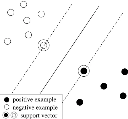
negative example positive example
[image:2.612.319.535.71.272.2]support vector
Figure 1: Hyperplane (solid) and Support Vectors
problem:
maximize
l X
i=1
i 1
2 l X
i;j=1
i
j y
i y
j K(x
i ;x
j )
subject to 8i:0 i
C and
l X
i=1
i y
i =0 :
The solution gives an optimal hyperplane, which is a decision boundary between the two classes. Figure 1 illustrates an optimal hyperplane and its support vec-tors.
3 Virtual Examples and Virtual Support Vectors
Virtual examples are generated from labeled exam-ples.1 Based on prior knowledge of a target task, the label of a generated example is set to the same value as that of the original example.
For example, in hand-written digit recognition, virtual examples can be created on the assumption that the label of an example is unchanged even if the example is shifted by one pixel in the four princi-pal directions (Sch¨olkopf et al., 1996; DeCoste and Sch¨olkopf, 2002).
Virtual examples that are generated from support vectors are called virtual support vectors (Sch¨olkopf
1
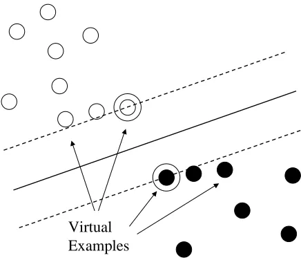
Virtual Examples
Figure 2: Hyperplane and Virtual Examples
et al., 1996). Reasonable virtual support vectors are expected to give a better optimal hyperplane. As-suming that virtual support vectors represent natu-ral variations of examples of a target task, the de-cision boundary should be more accurate. Figure 2 illustrates the idea of virtual support vectors. Note that after virtual support vectors are given, the hy-perplane is different from that in Figure 1.
4 Virtual Examples for Text Classification
We assume on text classification the following:
Assumption 1 The category of a document is
un-changed even if a small number of words are added or deleted.
This assumption is reasonable. In typical cases of text classification most of the documents usually contain two or more keywords which may indicate the categories of the documents.
Following Assumption 1, we propose two meth-ods to create virtual examples for text classification. One method is to delete some portion of a document. The label of a virtual example is given from the orig-inal document. The other method is to add a small number of words to a document. The words to be added are taken from documents, the label of which is the same as that of the document. Although one can invent various methods to create virtual exam-ples based on Assumption 1, we propose here very simple ones.
Document Id Feature Vector (x) Label (y)
1 (f
1 ;f
2 ;f
3 ;f
4 ;f
5
) +1
2 (f
2 ;f
4 ;f
5 ;f
6
) +1
3 (f
2 ;f
3 ;f
5 ;f
6 ;f
7
) +1
4 (f
1 ;f
3 ;f
8 ;f
9 ;f
10
) 1
5 (f
1 ;f
8 ;f
10 ;f
11
) 1
Table 1: Example of Document Set
Before describing our methods, we describe text representation which we used in this study. We to-kenize a document to words, downcase them and then remove stopwords, where the stopword list of freeWAIS-sf2 is used. Stemming is not performed. We adopt binary feature vectors where word fre-quency is not used.
Now we describe the two proposed methods: GenerateByDeletion and GenerateByAddition. As-sume that we are given a feature vector (a document)
xandx 0
is a generated vector fromx.
GenerateBy-Deletion algorithm is:
1. Copyxtox 0
.
2. For each binary feature f of x 0
, if rand()
t then remove the feature f, where rand() is
a function which generates a random number from0to1, andtis a parameter to decide how
many features are deleted.
For example, suppose that we have a set of docu-ments as in Table 1. Some possible virtual examples generated from Document 1 by GenerateByDeletion algorithm are (f
2 ;f
3 ;f
4 ;f
5
;+1), (f 1
;f 3
;f 4
;+1),
or(f 1
;f 2
;f 4
;f 5
;+1).
On the other hand, GenerateByAddition algo-rithm is:
1. Collect from a training set documents, the label of which is the same as that ofx.
2. Concatenate all the feature vectors (documents) to create an arrayaof features. Each element
ofais a feature which represents a word.
3. Copyxtox 0
.
2
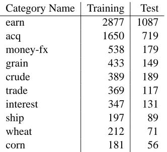
[image:3.612.315.537.71.157.2]Category Name Training Test
earn 2877 1087
acq 1650 719
money-fx 538 179
grain 433 149
crude 389 189
trade 369 117
interest 347 131
ship 197 89
wheat 212 71
[image:4.612.104.270.70.221.2]corn 181 56
Table 2: Number of Training and Test Examples
4. For each binary featuref ofx 0
, if rand() t
then select a feature randomly fromaand put
it tox 0
.
For example, when we want to generate a virtual example from Document 2 in Table 1 by Generate-ByAddition algorithm, first we create an arraya =
(f 1 ;f 2 ;f 3 ;f 4 ;f 5 ;f 2 ;f 4 ;f 5 ;f 6 ;f 2 ;f 3 ;f 5 ;f 6 ;f 7 ).
In this case, some possible virtual examples by GenerateByAddition are (f
1 ;f 2 ;f 4 ;f 5 ;f 6 ;+1),
(f 2 ;f 3 ;f 4 ;f 5 ;f 6
;+1), or (f 2 ;f 4 ;f 5 ;f 6 ;f 7
;+1).
An example such as(f 2 ;f 4 ;f 5 ;f 6 ;f 10
;+1)is never
generated from Document 2 because there are no positive documents which havef
10.
5 Experimental Results and Discussion
5.1 Test Set Collection
We used the Reuters-21578 dataset3 to evaluate the proposed methods. The dataset has several splits of a training set and a test set. We used here “ModApte” split, which is most widely used in the literature on text classification. This split has 9,603 training ex-amples and 3,299 test exex-amples. More than 100 cat-egories are in the dataset. We use, however, only the most frequent 10 categories. Table 2 shows the 10 categories and the number of training and test exam-ples in each of the categories.
5.2 Performance Measures
We use F-measure (van Rijsbergen, 1979; Lewis and Gale, 1994) as a primal performance measure
3
Available from David D. Lewis’s page: http://
www.daviddlewis.com/resources/testcollections/reuters21578/
to evaluate the result. F-measure is defined as:
F-measure = (1+ 2 )pq 2
p+q
(4)
wherepis precision andqis recall andis a
param-eter which decides the relative weight of precision and recall. Thepand theqare defined as:
p =
number of positive and correct outputs number of positive outputs
q =
number of positive and correct outputs number of positive examples
In Equation 4, usually = 1is used, which means
it gives equal weight to precision and recall.
When we evaluate the performance of a classifier to a multiple category dataset, there are two ways to compute F-measure: macro-averaging and micro-averaging (Yang, 1999). The former way is to first compute F-measure for each category and then aver-age them, while the latter way is to first compute pre-cision and recall for all the categories and use them to calculate the F-measure.
5.3 SVM setting
Through our experiments we used our original SVM tools, the algorithm of which is based on SMO (Se-quential Minimal Optimization) by Platt (1999). We used linear SVMs and set a misclassification costC
to0:016541which is1=(the average ofxx)where
xis a feature vector in the 9,603 size training set.
For simplicity, we fixed C through all the
experi-ments. We built a binary classifier for each of the 10 categories shown in Table 2.
5.4 Results
First, we carried out experiments using GenerateBy-Deletion and GenerateByAddition separately to cre-ate virtual examples, where a virtual example was created per Support Vector. We did not generate virtual examples from non support vectors. We set the parametertto0:05
4for GenerateByDeletion and
GenerateByAddition for all the experiments. To build an SVM with virtual examples we use the following steps:
4
We first triedt =0:01;0:05;and0:10with
GenerateBy-Deletion using the 9603 size training set. The valuet=0:05
1. Train an SVM.
2. Extract Support Vectors.
3. Generate virtual examples from the Support Vectors.
4. Train another SVM using both the original la-beled examples and the virtual examples.
We evaluated the performance of the two methods depending on the size of a training set. We created subsamples by selecting randomly from the 9603 size training set. We prepared seven sizes: 9603, 4802, 2401, 1200, 600, 300, and 150.5 Micro-average F-measures of the two methods are shown in Table 3. We see from Table 3 that both the meth-ods give better performance than that of the origi-nal SVM. The smaller the number of examples in the training set is, the larger the gain is. For the 9603 size training set, the gain of GenerateByDele-tion is 0.75 (= 90:17 89:42), while for the 150
size set, the gain is 6.88 (= 60:16 53:28). These
results suggest that in the smaller training sets there are not enough various examples to give a accurate decision boundary and therefore the effect of virtual examples is larger at the smaller training sets. It is reasonable to conclude that GenerateByDeletion and GenerateByAddition generated good virtual ex-amples for the task and this led to the performance gain.
After we found that the simple two methods to generate virtual support vectors were effective, we examined a combined method which is to use both GenerateByDeletion and GenerateByAddition. Two virtual examples are generated per Support Vector. The performance of the combined method is also shown in Table 3. The performance gain of the com-bined method is larger than that with either Gener-ateByDeletion or GenerateByAddition.
Furthermore, we carried out another experiment with a combined method to create two virtual exam-ples with GenerateByDeletion and GenerateByAd-dition respectively. That is, four virtual examples were generated from a Support Vector. The perfor-mance of that setting is shown in Table 3. The best
5
Since we selected samples randomly, some smaller training sets of low frequent categories may have had few or even zero positive examples.
50 55 60 65 70 75 80 85 90 95
100 1000 10000
Micro-average F-measure (beta = 1)
[image:5.612.321.533.74.224.2]Number of Examples in Training Set SVM + 4 Virtual SVs Per SV SVM
Figure 3: Micro-Average F-Measure versus Number of Examples in the Training Set
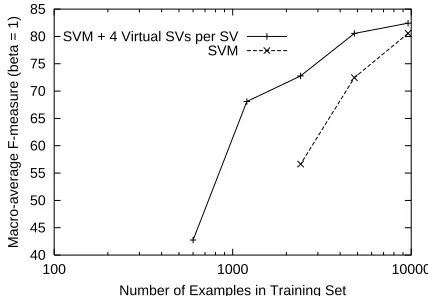
40 45 50 55 60 65 70 75 80 85
100 1000 10000
Macro-average F-measure (beta = 1)
Number of Examples in Training Set SVM + 4 Virtual SVs per SV
SVM
Figure 4: Macro-Average F-Measure versus Num-ber of Examples in the Training Set. For the smaller training sets F-measures cannot be computed be-cause the precisions are undefined.
result is achieved by the combined method to create four virtual examples per Support Vector.
[image:5.612.318.532.288.436.2]Number of Examples in Training Set
Method 9603 4802 2401 1200 600 300 150
Original SVM 89.42 86.58 81.69 77.24 71.08 64.44 53.28
[image:6.612.66.542.72.168.2]SVM + 1 VSV per SV (GenerateByDeletion) 90.17 88.62 84.45 81.11 75.32 70.11 60.16 SVM + 1 VSV per SV (GenerateByAddition) 90.00 88.51 84.48 81.14 75.33 69.59 60.04 SVM + 2 VSVs per SV (Combined) 90.27 89.33 86.27 83.59 77.44 72.81 64.22 SVM + 4 VSVs per SV (Combined) 90.45 89.69 87.12 84.97 79.16 73.25 65.05
Table 3: Comparison of Micro-Average F-measure of Different Methods. “VSV” means virtual SV.
1 2 3 4 5 6
100 1000 10000
Error Rate (%)
Number of Examples in Training Set SVM + 4 Virtual SVs per SV
SVM
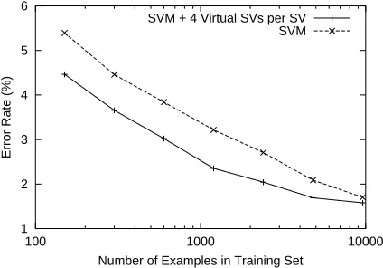
Figure 5: Error Rate versus Number of Examples in the Training Set
is realized simply because the recall gets highly improved while the error rate increases. We plot changes of the error rate for 32990 tests (3299 tests for each of the 10 categories) in Figure 5. SVM with 4 VSVs still outperforms the original SVM signifi-cantly.6
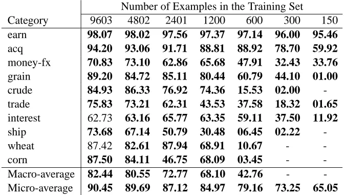
The performance changes for each of the 10 cat-egories are shown in Tables 4 and 5. SVM with 4 VSVs is better than the original SVM for almost all the categories and all the sizes except for “inter-est” and “wheat” at the 9603 size training set. For low frequent categories such as “ship”, “wheat” and “corn”, the classifiers of the original SVM perform poorly. There are many cases where they never out-put ‘positive’, i.e. the recall is zero. It suggests that the original SVM fails to find a good hyperplane due to the imbalanced training sets which have very few
6
We have done the significance test which is called “p-test” in (Yang and Liu, 1999), requiring significance at the 0.05 level. Although at the 9603 size training set the improvement of the error rate is not statistically significant, in all the other cases the improvement is significant.
positive examples. In contrast, SVM with 4 VSVs yields better results for such harder cases.
6 Conclusion and Future Directions
We have explored how virtual examples improve the performance of text classification with SVMs. For text classification, we have proposed methods to cre-ate virtual examples on the assumption that the label of a document is unchanged even if a small num-ber of words are added or deleted. The experimen-tal results have shown that our proposed methods improve the performance of text classification with SVMs, especially for small training sets. Although the proposed methods are not readily applicable to NLP tasks other than text classification, it is notable that the use of virtual examples, which has been very little studied in NLP, is empirically evaluated.
In the future, it would be interesting to employ virtual examples with methods to use both labeled and unlabeled examples (e.g., (Blum and Mitchell, 1998; Nigam et al., 1998; Joachims, 1999)). The combined approach may yield better results with a small number of labeled examples. Another interest-ing direction would be to develop methods to create virtual examples for the other tasks (e.g., named en-tity recognition, POS tagging, and parsing) in NLP. We believe we can use prior knowledge on these tasks to create effective virtual examples.
References
Avrim Blum and Tom Mitchell. 1998. Combining la-beled and unlala-beled data with co-training. In
Proceed-ings of the 11th COLT, pages 92–100.
[image:6.612.80.292.218.366.2]Number of Examples in the Training Set
Category 9603 4802 2401 1200 600 300 150
earn 98.06 97.49 97.40 96.39 95.94 94.85 93.73 acq 91.94 89.87 84.43 84.01 78.17 63.10 12.03 money-fx 64.90 61.69 56.03 51.69 17.91 01.11 05.38 grain 86.96 81.68 75.20 59.63 41.27 06.49 -crude 84.59 81.52 67.11 33.33 01.05 - -trade 74.89 64.58 54.86 40.26 12.80 01.69 -interest 63.89 60.29 50.27 35.15 08.57 05.88
-ship 66.19 44.07 32.73 02.22 - -
-wheat 89.61 80.60 38.30 08.11 - -
-corn 84.62 62.79 10.17 - - -
[image:7.612.142.474.109.298.2]-Macro-average 80.56 72.46 56.65 - - - -Micro-average 89.42 86.58 81.69 77.24 71.08 64.44 53.28
Table 4: F-Measures for the Reuters Categories with the Original SVM. The hyphen ‘-’ denotes the case where F-measure cannot be computed because the classifier always says ‘negative’ and therefore its preci-sion is undefined. The scores in bold means that the score of the original SVM is better than that of SVM with 4 Virtual SVs per SV (shown in Table 5).
Number of Examples in the Training Set
Category 9603 4802 2401 1200 600 300 150
earn 98.07 98.02 97.56 97.37 97.14 96.00 95.46
acq 94.20 93.06 91.71 88.81 88.92 78.70 59.92
money-fx 70.83 73.10 62.86 65.68 47.91 32.43 33.76
grain 89.20 84.72 85.11 80.44 60.79 44.10 01.00
crude 84.93 86.33 76.92 74.36 15.53 02.00 -trade 75.83 73.21 62.31 43.53 37.58 18.32 01.65
interest 62.73 63.16 65.77 63.35 59.11 37.50 11.92
[image:7.612.138.475.442.632.2]ship 73.68 67.14 50.79 30.48 06.45 02.22 -wheat 87.42 82.61 87.94 68.91 10.67 - -corn 87.50 84.11 46.75 68.09 03.45 - -Macro-average 82.44 80.55 72.77 68.10 42.76 - -Micro-average 90.45 89.69 87.12 84.97 79.16 73.25 65.05
Susan Dumais, John Platt, David Heckerman, and Mehran Sahami. 1998. Inductive learning algorithms and representations for text categorization. In
Pro-ceedings of the ACM CIKM International Conference on Information and Knowledge Management, pages
148–155.
Thorsten Joachims. 1998. Text categorization with sup-port vector machines: Learning with many relevant features. In Proceedings of the European Conference
on Machine Learning, pages 137–142.
Thorsten Joachims. 1999. Transductive inference for text classification using support vector machines. In
Proceedings of the 16th International Conference on Machine Learning, pages 200–209.
Taku Kudo and Yuji Matsumoto. 2001. Chunking with support vector machines. In Proceedings of NAACL
2001, pages 192–199.
Taku Kudo and Yuji Matsumoto. 2002. Japanese depen-dency analysis using cascaded chunking. In
Proceed-ings of CoNLL-2002, pages 63–69.
David D. Lewis and William A. Gale. 1994. A sequential algorithm for training text classifiers. In Proceedings
of the Seventeenth Annual International ACM-SIGIR Conference on Research and Development in Informa-tion Retrieval, pages 3–12.
Kamal Nigam, Andrew McCallum, Sebastian Thrun, and Tom Mitchell. 1998. Learning to classify text from labeled and unlabeled documents. In Proceedings of
the Fifteenth National Conference on Artificial Intelli-gence (AAAI-98), pages 792–799.
Partha Niyogi, Federico Girosi, and Tomaso Poggio. 1998. Incorporating prior information in machine learning by creating virtual examples. In Proceedings
of IEEE, volume 86, pages 2196–2207.
John C. Platt. 1999. Fast training of support vec-tor machines using sequential minimal optimization. In Bernhard Sch¨olkopf, Christopher J.C. Burges, and Alexander J. Smola, editors, Advances in Kernel
Meth-ods: Support Vector Learning, pages 185–208. MIT
Press.
Manabu Sassano. 2002. An empirical study of active learning with support vector machines for Japanese word segmentation. In Proceedings of ACL-2002, pages 505–512.
Bernhard Sch¨olkopf, Chris Burges, and Vladimir Vap-nik. 1996. Incorporating invariances in support vector learning machines. In C. von der Malsburg, W. von Seelen, J.C. Vorbr¨uggen, and B. Sendhoff, editors,
Ar-tificial Neural Networks – ICANN’96, Springer Lec-ture Notes in Computer Science, Vol. 1112, pages 47–
52.
Cynthia A. Thompson, Mary Leaine Califf, and Ray-mond J. Mooney. 1999. Active learning for natural language parsing and information extraction. In
Pro-ceedings of the Sixteenth International Conference on Machine Learning, pages 406–414.
C.J. van Rijsbergen. 1979. Information Retrieval. But-terworths, 2nd edition.
Vladimir N. Vapnik. 1995. The Nature of Statistical
Learning Theory. Springer-Verlag.
Yiming Yang and Xin Liu. 1999. A re-examination of text categorization methods. In Proceedings of
SIGIR-99, 2nd ACM International Conference on Research and Development in Information Retrieval, pages 42–
49.
Yiming Yang. 1999. An evaluation of statistical ap-proaches to text categorization. Journal of
Informa-tion Retrieval, 1(1/2):67–88.
David Yarowsky. 1995. Unsupervised word sense dis-ambiguation rivaling supervised methods. In