Support vector machines for texture classification

Support Vector Machines for

Texture Classification

Kwang In Kim, Keechul Jung, Se Hyun Park, and

Hang Joon Kim

Abstract—This paper investigates the application of support vector machines (SVMs) in texture classification. Instead of relying on an external feature extractor, the SVM receives the gray-level values of the raw pixels, as SVMs can generalize well even in high-dimensional spaces. Furthermore, it is shown that SVMs can incorporate conventional texture feature extraction methods within their own architecture, while also providing solutions to problems inherent in these methods. One-against-others decomposition is adopted to apply binary SVMs to multitexture classification, plus a neural network is used as an arbitrator to make final classifications from several one-against-others SVM outputs. Experimental results demonstrate the effectiveness of SVMs in texture classification.

Index Terms—Support vector machines, texture analysis, pattern classification, machine learning, feature extraction.

æ

1

I

TEXTUREclassification is basically the problem of classifying pixels in an image according to their textural cues. This is different from conventional image segmentation as the texture is characterized using both the gray value for a given pixel and the gray-level pattern in the neighborhood surrounding the pixel. Crucial to the success of texture classification are 1) the identification of features that differentiate textures in an image and developing their representations for further classification and 2) the construction of classification paradigms that operate on the above representa-tions and discriminate between texture features associated with different texture classes. Accordingly, the texture classification problem is conventionally divided into the two subproblems of feature extraction and classification [1], [2], [3].

Many methods have been developed to extract textural features, which can loosely be classified as statistical, model-based, and signal processing methods. In statistical approaches, textures are described using statistical measures, such as the co-occurrence or autocorrelation statistics of the gray levels fork-tuplesof pixels [4], [5]. The major drawback to this type of method is the enormous amount of data involved inkthorder statistics, which is especially hard to handle when k is large (k >2). This is relevant as psychophysical experiments have demonstrated that the human visual system is able to extract some statistics of an order higher than two [6]. Model-based methods characterize texture images based on probability distributions in random fields, such as Markov chains and Markov random fields (MRFs) [7], [9], [20], [30]. MRFs are widely used because they yield a local and economical texture

description [7]. However, they also require intensive computation to determine the proper parameters [8]. Signal processing methods, also known as multichannel filtering methods, are attractive due to their simplicity [9]. In these methods, a textured input image is decomposed into feature images using a bank of filters, such as Gabor, wavelet, or neural network-based filters [10], [11], [12]. As a result, a high-dimensional textural pattern can be represented by a relatively small set of feature statistics that need to be extracted using a set of well-selected filters. Therefore, the major issue for this type of method is the selection of a good set of filters for a given texture classification problem.

From Bayes classifiers to neural networks, there are many possible choices for an appropriate classifier. Among these, support vector machines (SVMs) would appear to be a good candidate because of their ability to generalize in high-dimensional spaces, such as spaces spanned by texture patterns. The appeal of SVMs is based on their strong connection to the underlying statistical learning theory. That is, an SVM is an approximate implementation of the structural risk minimization (SRM) method [13]. For several pattern classification applications, SVMs have already been shown to provide better generalization performance than traditional techniques, such as neural networks [14], [15].

The aim of this paper is to illustrate the potential of SVMs in texture classification. Accordingly, a method for texture classifica-tion using SVMs is described. Unlike other texture classificaclassifica-tion methods, the proposed method does not externally incorporate any of the abovementioned feature extraction methods. Instead, the gray-level values of the raw pixels are directly fed to the SVM. The only preprocessing of the input before feeding it to the SVM is the selection of certain pixels following the configuration of autoregressive (AR) features. As a result, both feature extraction and classification are performed within the SVM architecture. The proposed method is based on the observation that an SVM incorporates feature extractors, therefore, nonlinear mapped input patterns can be used as feature vectors. Actually, in an SVM, feature extraction is implicitly performed by a kernel, which is defined as the dot product of two mapped patterns. It is also shown that one kernel (called a polynomial kernel) can perform the same operations as conventional feature extraction methods (specifically, statistical feature extraction and multichannel filter-ing). Furthermore, SVMs with such a kernel can provide solutions to the problems inherent in conventional feature extraction methods. The main advantage of the proposed method is that there is no need for a carefully designed feature extraction mechanism because the feature extraction task is reduced to the problem of training the SVMs. Thereafter, feature extraction and classification are both performed in accordance with a unique criterion referred to as theclassification rate.

Since SVMs were originally developed for two-class problems, their basic scheme is extended to multitexture classification by adopting theone-against-othersdecomposition method. This works by applying SVMs that first separate one class from all the other classes, and then arbitrating between several SVMs. A neural network is used as the arbitrator and the results are compared with the commonly usedmax-selection scheme. The proposed method was tested using several Brodatz and MIT Vision Texture images. The excellent classification rates achieved in the experiments confirm that SVMs are well-suited for texture classification.

2

O

SVM

An SVM constructs a binary classifier from a set of labeled patterns calledtraining examples. Letðxi; yiÞ 2RN f 1g,i¼1;. . .; lbe such

a set of training examples. The purpose is to select the function f:RN! f 1gfrom a given class of functionsff:2gsuch

thatfwill correctly classify test examplesðx; yÞ. If no restriction is placed on the class of functions when choosing the estimatef, even a function that performs well with training data may not generalize well to unseen examples. Hence, just minimizing the training error . K.I. Kim is with the Artificial Intelligence Lab, Computer Science

Department, Korea Advanced Institute of Science and Technology, Taejon, 305-701, Korea. E-mail: [email protected].

. K. Jung is with the Pattern Recognition and Image Processing Lab, Computer Science and Engineering Department, 3115 Engineering Bldg., Michigan State University, MI 48824-1226. E-mail: [email protected]. . S.H. Park is with the Computer Engineering Division, College of

Electronics and Information, Chosun University, Gwangju, 501-759, Korea. E-mail: [email protected].

. H.J. Kim is with the Computer Engineering Department, Kyungpook National University, Taegu, 702-701, Korea.

E-mail: [email protected].

Manuscript received 31 May 2000; revised 14 June 2001; accepted 21 Feb. 2002.

Recommended for acceptance by A. Kundu.

For information on obtaining reprints of this article, please send e-mail to: [email protected], and reference IEEECS Log Number 112204.

As such, this theory provides bounds for the test error. The minimization of these bounds, which depend on both the empirical risk and the capacity of the function class, leads to the principle of

structural risk minimization (SRM) [13], [16]. The best-known

capacity concept of this theory is the VC-dimension, defined as the largest number of points that can be separated in all possible ways using the functions of the given class [13].

To design learning algorithms, the capacity of the class of functions selected needs to be computed. The SVM selects the class of separating hyperplanes whose VC-dimension bounds can be computed and then identifies the optimal separating hyperplane (OSH) that maximizes the margin of the nearest examples. This is equivalent to minimizing the VC-dimension bound. The OSH is then computed as a decision surface of the form:

fð Þ ¼x sgn X ls

i¼1

yiixsixþb

!

; ð1Þ

where xs i

ls

i¼1is a subset of the training data set. These subsets are

calledsupport vectors(SVs) and are the points from the data set that fall closest to the separating hyperplane. The coefficientsiandbare

determined by solving the large-scale quadratic programming problem:

Maximize

W ð Þ ¼X

l

i¼1

iÿ 1 2

Xl

i;j¼1

ijyiyj xixj

ÿ

subject to the constraints:

Xl

i¼1

iyi¼0; 0iC fori¼1;. . .; l:

The parameterCcan be regarded as the regularization parameter and is selected by the user. A largerCcorresponds to assigning a higher penalty to the training errors.

However, since it is unlikely that a general pattern recognition problem can actually be solved by a linear classifier (separating hyperplane), the OSH needs to be augmented in order to allow for nonlinear decision surfaces. The basic idea is to map the data into another dot product space (called the feature space) F via a nonlinear map :RN _{!F and perform the above linear}

algo-rithm inF. Since the solution has the form

fð Þ ¼x sgn X ls

i¼1

yiið Þxsið Þ þx b

!

; ð2Þ

it is nonlinear in the original input variables.

The mapping is performed in accordance with Cover’s theorem on the seperability of patterns [17]. Consider a space made up of nonlinearly separable patterns. Cover’s theorem states that such a multidimensional space can be transformed into a new

This introduces the important problem of how to treat such high-dimensional space computationally. This can be resolved based on two observations: First, although some mappings have very high dimensionalities, their inner products can be easily computed, and second, all themappings used in the SVM occur in the form of an inner product. Accordingly, the solution is to replace all the occurrences of an inner product resulting from two mappings with the kernel functionKdefined as:

Kðx;yÞ ¼ð Þ x ð Þy:

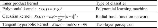
Conversly, given a symmetric positive kernel Kðx;yÞ, Mercer’s theorem [29] implies the existance of a mapping such that Kðx;yÞ ¼ð Þ x ð Þy. Then, without considering the mapping explicitly, a nonlinear SVM can be constructed by selecting the proper kernel. Table 1 summarizes the kernel functions for three common types of SVMs: polynomial learning machines, radial basis function networks (RBFNs), and two-layer perceptrons [13], [16].

3

T

C

U

S

V

M

This section describes the classification system devised to assess the potential of SVMs in texture classification. First, some useful properties of SVMs for texture classification are discussed in Section 3.1. Based on these properties, Section 3.2 outlines the representation of texture patterns from an input image and introduces an SVM classifier for a two-class texture classification problem. Section 3.3 describes the SVM-neural network architec-ture for more general multiclass texarchitec-ture classification problems. Finally, the postprocessing method is presented in Section 3.4.

3.1 Optimality of SVMs for Texture Classification

The operation of an SVM for texture classification is two-fold:

1. The nonlinear mapping of a texture space into a possibly high-dimensional feature space.

2. The construction of an OSH in the feature space.

Step 2 is explained in Section 2. Therefore, the current section discusses the optimality of Step 1 for texture representations i.e., texture feature extraction, from two different perspectives:

. Statistical feature extraction.By introducing various kernel functions (for example, see Table 1), variousmappings can be used, which are implicitly imbedded in the SVMs. One of these mappings (induced by a polynomial kernel) takes thep-ordercorrelations between the entriesxiof the

comprising a feature spaceFof dimensionalityNF. As such,

a1717texture pattern and monomial degreep¼5yield a feature space dimensionality of about 108_{. However,}

introducing a polynomial kernel facilitates work in such a space, as a polynomial kernel with degreepcorresponds to the dot product of the feature vectors extracted by the monomial feature extractorCp[13]:

Cpð Þ x Cpð Þy

ÿ

¼ X

N

i1;...;ip¼1

xi1. . .xipyi1. . .yip

¼ X

N

i¼1

xiyi

!p

¼ðxyÞp:

. Signal processing. In multichannel filtering methods, a textured input image is decomposed into a set of feature images using a bank of filters. The decomposition is accomplished by filtering the input image, applying a nonlinear function to all the pixels in the filtered images, and spatially smoothing each output image [10]. The channels corresponding to different filters are assumed to capture certain specific local characteristics of the input texture, such as the spatial frequency, directionality, edge-ness, etc. Yet, the major issue in multichannel filtering is the filter selection problem: That is, the selection of a moderate number of filters that can capture the textural properties of the given classification problem. This filter selection problem has been tackled both empirically [18] and theoretically [19], [20]. However, the practical implementa-tion of both types of soluimplementa-tion, tend to be computaimplementa-tionally prohibitive, or result in a suboptimal solution. The opera-tion performed by a kernel in an SVM is essentially the same as that of a channel in a multichannel filtering method: The kernel first computes the inner productz¼xybetween its input x and the SVs y and then performs a nonlinear transformation. In the case of a polynomial kernel, this transformation corresponds to a polynomial function

ð Þ ¼z ð Þzp

ð Þ. The only difference is that the spatial smoothing of the feature values is omitted, as in the proposed method, this is performed in a postprocessing stage. In the new method, the SVs play the role of a filter bank. Even though they are not designed as filters for capturing specific frequency bands or orientations, they can still extract critical measures for classification. As such, it should be noted that an SVM can emphasize the correct separation of training data through the selection of filters

(SVs), while, in a classical multichannel filtering approach, the filter selection criteria are generally not directly related to classification performance. In this respect, an SVM texture classifier is rather similar to a neural network-based multichannel filtering method [12]. However, in contrast to a neural network, an SVM is more concerned with minimizing the test error than with directly minimizing the training error. Futhermore, in an SVM, the number of filters and their coefficients are both automatically deter-mined by the number of SVs and their values, respectively. By selecting the SVs as special-purpose filters optimized for given textures, the SVM can automatically identify an optimal feature extractor and the corresponding texture classifier based on a unified criterion of minimizing the test error for a given texture classification task.

3.2 Data Representation and Classification of Two-Class Textures

The simplest way to characterize the variability in a texture pattern is by noting the gray-level values of the raw pixels. This set of gray values becomes the feature set on which the classification is based. An important advantage of this approach is the speed with which images can be processed, as the features do not need to be calculated. However, the main disadvantage is that the size of the feature vector is large. Accordingly, a texture classifier may need to generalize texture patterns in a high-dimensional space. SVMs are the proper tool for this problem because they are capable of learning in sparse and high-dimensional spaces with very few training examples. Furthermore, SVMs themselves incorporate feature extractors and can use their nonlinear mapped input

their features on a different user-defined feature set.

Fig. 1 shows the architecture of an SVM texture classifier, which involves three layers with entirely different roles. The input layer is made up of source nodes that connect the SVM to its environment. Its activation xcomes directly from the gray-level values of the MM window in the input image. However, instead of using all the pixels in the window, the input configuration for extracting AR features (only the shaded pixels from the input window in Fig. 1) [9] is used. This reduces the size of the feature vector from M2 _{to 4M-3, thereby resulting in an}

improved generalization performance and classification speed. The hidden layer applies a nonlinear transformation from the input space to the feature spaceF, where the inner products are computed. These two operations are in practice performed in a single step using the kernel function. The size of the hidden layer mis determined as the number of SVs identified by the SVM. It should also be noted that the SVs help shape and better define the decision surface, when compared with other patterns and are border patterns from a geometrical point of view. Consequently, since there are usually very few SVs, the size of the hidden layer is moderate. The output layer is a hyperplane classifier, supplying the response of the network to the activation pattern applied to the input layer. The sign of the SVM outputyrepresents the class of the central pixel in the input window.

The parameters that need to be tuned in the SVMs include the kernel parameters and regularization parameterC. One straight-forward method for tuning is to use validation data, which are distinct from the training data. However, when the amount of available training data is limited, it is important to have an alternative means of tuning the parameters, without having to put aside parts of the training set for validation purposes. The proposed method for tuning the parameters is mainly based on Scho¨lkopf et. al’s work [21].

The strength of an SVM is based in its automatic capacity control (in terms of the VC-dimension). This capacity control takes place within a class of functions ff:2g specified a priori by the

choice of the kernel function (or equivalentlyF). Scho¨lkopf et. al pointed out that the VC-dimension offcan be estimated by a term

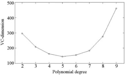
that is in proportion to the radiusrof the smallest ball containing all the data points inF [21]. Sincerdepends on the shape ofF, the VC-dimension depends on the kernel parameters (p, in the case of a polynomial kernel). The estimation of r from the given kernel parameters can be formulated in a similar way to training SVMs [21]. The VC-dimension and training errors can then be compared to select the optimal kernel parameters. The proposed strategy is to select those parameters that minimize r, while retaining a zero

the classification of several texture images have shown that the training error diminishes whenp4. However, for more complex problems, this condition could be relaxed. For the same reason, parameterCdoes not have a significant effect on the classification because, in the case of a zero training error, it is not included in the computation of the OSH. Accordingly, aCvalue of 100 was used in the current study for training the SVMs. Readers interested in the automatic selection ofCare referred to [22].

A two-class texture classification problem was considered as an example (Fig. 3a). SVMs with a varying p were trained with 2,000 training examples obtained using random selections of 1,000 patterns from both classes. The input window size was fixed at 1717. The estimated VC-dimensions and training errors for different degrees are shown in Fig. 2 and Table 2. From the results, the optimal degree for this problem was determined to be 5, which exhibited the minimal VC-dimension and produced zero training errors.

3.3 Multiclass Texture Classification

The previous section described an SVM for a two-class texture classification problem, called a dichotomy. This may also be appropriate for texture-based object detection applications when discriminating an object from the background. However, the majority of texture classification problems involve more than two textures. Consequently, extended SVMs are required for applica-tion to multiple textures, and the optimal design of multiclass SVM classifiers is still an area of active research. One frequently used method is one-against-others decomposition, which works by constructing an SVM !r for each classrthat first separates that

class from all the other classes and then uses an expert F to arbitrate between each SVM output in order to produce the final decision. The effectiveness of this method in the problem of texture classification has already been demonstrated using HMM-based classifiers [23].

A max-selector is the simplest form of arbitrator. If g¼

g1_{;. . .; g}R

ÿ T

denotes the output1 of a system of R one-against-others SVMs, themax-selectorpicks classrfor the inputx, which then maximizesgr_{as defined by}

F¼arg max r ðgÞ:

However, a max-selector suffers from a scaling problem because it assumes that all thegs are on the same scale, which is not the case for SVMs. If the SVM is trained to produce outputs for the SVs as 1, the scale is not robust as it only depends on a few data, often including outliers [24]. In a max-selector, the output class is determined by choosing the maximum of all the SVM outputs. However, the outputs of the remaining SVMs, other than the winner, also carry certain information. Moreover, the mean ofg can vary significantly according to the class of input [24]. This TABLE 2

Training Errors for Fig. 3a as a Function ofp

knowledge can be used to improve the overall recognition performance. In [24], a stacking technique based on linear mapping was applied for normalizing g. While this technique shows significant improvements over the bare one-against-others decom-position, preliminary experiments have indicated that a linear normalization is often insufficient for texture classification as the relation amonggs becomes nonlinear. In the current work, after uniformly scaling g by applying a tangent hyperbolic function h¼ðh;. . .; hÞT

, a nonlinear mapping M:RR_!RR _{is used to}

aggregate the answers of all the SVMs into a score for each class. Thus, the arbitrator can be defined by

F¼arg max

r ðMðh gð ÞÞÞ:

A two-layer neural network, composed of a size 2 hidden layer with a tangent hyperbolic activation function, is adopted for the mapping M. The network is designed to minimize the mean square error betweenh g xð ð ÞÞand the desired outputy¼ ÿð 1;. . .;þ1;. . .ÿ1ÞT and trained using a back-propagation algorithm.

3.4 Postprocessing

Any method can result in a classification error. In the proposed method, misclassified pixels usually take the form of noisy speckles scattered across the entire classification image. In this case, simple image smoothing techniques can reduce the error rate by an order of magnitude. In the current study, two-dimensional median filtering with a window size of five was used for postprocessing the classified image. The application of this method improved the error rate by an average of 7 percent. However, it is worth noting that the error rate created by a smoothing technique may depend on the size and shape of the uniformly textured regions.

4

E

R

To verify the effectiveness of the proposed method, experiments were performed on a supervised segmentation of several test images. The test images were drawn from two different commonly

used texture sources: the Brodatz album [25] and MIT Vision Texture (VisTex) database [26] (See Figs. 3 and 4). Table 3 summarizes the sources of the test images.

All textures were originally gray-scale images with 256 levels. The texture classifier was trained on randomly selected portions of 256256 subimages of texture images that were not included in the test images. To make the textures indiscriminable for the local mean gray level or local variance, both the training and test images were globally histogram-equalized before being used and the gray scales linearly normalized into½ÿ1;1Š. The desired classes for the patterns were then manually assigned. Patterns lying on the texture boundaries were excluded from the training set due to the difficulties involved in manually assigning the desired value for the training pattern. Accordingly, this introduced a tradeoff when choosing the appropriate window size for the classification accuracy of uniform texture regions and texture boundaries, as the shape and size of the texture boundaries and input window size all affect the performance of the classification method. Therefore, the experiments were performed with different input window sizes of55,99,1313,1717, and2121.

Polynomial kernels were emphasized because of their relevance to conventional feature extraction methods, yet the performance of the SVMs with other kernels, including a linear SVM (with a polynomial kernel of degree 1), was also tested. All the experiments were performed using a 500 MHz Pentium3 CPU. The time spent classifying an image depended on the number of texture classes (equal to the number of SVMs), input window size, type of kernels, and number of SVs. It took about one minute to classify the entire image of Fig. 3a using a degree-5 polynomial kernel and 1717window.

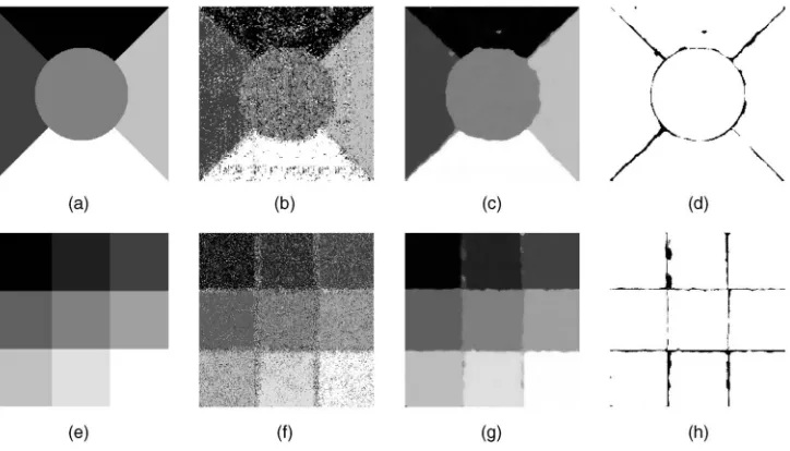
4.1 Two-Texture Images

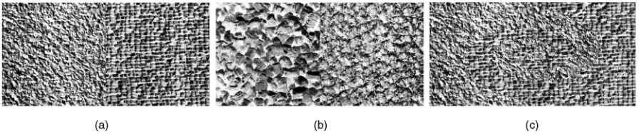
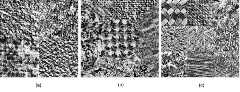
The sizes of the images in Fig. 3 are512256and the size of each textured subregion is half that of the test image. The sources of the texture classes in Fig. 3c are the same as those in Fig. 3a. However, since the texture boundary in Fig. 3c is more complex and larger than that in Fig. 3a, a larger window size was considered to be disadvantageous for classifying Fig. 3c, when compared with Fig. 3a. The training data set was obtained by randomly selecting Fig. 4. Multitexture images used in experiments.

1,000 patterns from each texture. This corresponded to about 1.7 percent of the total available input patterns.

To evaluate the effect of the polynomial degreepon the texture classification performance, a set of experiments was performed with varying degrees of p. The input window size was fixed at 1717. Table 4 shows the error rates and numbers of SVs for the classification of Figs. 3a and 3b. The highest recognition rates were obtained using degree-7 and -9 polynomial kernels. However, no obvious optimum was identified. Higher degrees ofpafforded a low error rate, while a saturation point was reached whenp5. Although not optimal in testing, a degree-5 polynomial kernel for Fig. 3a, estimated from the training set (see Section 3.2), was identified as second best, which was only slightly behind the best (0.1 percent). For a degree-1 polynomial kernel (i.e., linear SVM), the problem was not separable and the error rate was rather high. In this case, all the training errors were related to the SVs, thereby causing a larger number of SVs. The number of SVs only slightly increased with an increasing polynomial degree. When compared with the number of training patterns, the relatively large number of SVs revealed that the texture-learning task for Fig. 3b was rather difficult to solve. Since no significant difference was observed

across the classification results when p5, a fixed value of five was used forpin the rest of the experiments.

The error rates according to the various window sizes are summarized in Table 5. The tendency for a smaller error rate was observed with larger input window sizes, except for a 2121window. The 1717window exhibited the best overall performance for the images in Figs. 3a and 3b. For more complex texture boundaries (Fig. 3c), the unstable classification of those patterns lying on the texture boundaries resulted in a larger error rate for a1717window. For comparison, classification results using Gaussian kernels and tangent hyperbolic kernels are also presented, where the parameters (¼0:5for Gaussian kernels and¼1:5for tangent hyperbolic kernels) were empirically selected. The highest recognition rates were obtained when using a polynomial kernel. The Gaussian kernels were slightly outperformed by the polynomial kernels, whereas the tangent hyperbolic kernels produced much higher error rates.

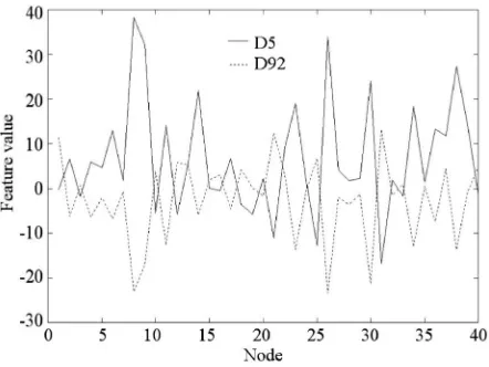
It should be noted that Fig. 3b was very difficult to discriminate for several texture feature extraction approaches, including Laws filters (a bank of band pass filters [28]), optimal representation Gabor filters, etc. [9], whereas an SVM with a polynomial kernel resulted in a rather low error rate. This demonstrates the usefulness of a monomial feature extractor induced by a polynomial kernel. Since it is not easy to visualize the feature space when the polynomial degree is larger than 2, the operation of this space was indirectly observed through the kernel responses (activation of hidden layer in Fig. 1). Fig. 5 shows the first 40 components of the average kernel responses calculated from each texture class (D5, D92). The distinct signatures observed from each texture class highlight the role of the hidden layer as a discriminative feature extractor for a given texture classification problem. It should also be noted that the operation of the hidden layer is essentially the same as that of a multichannel filtering scheme (see Section 3.1).

Fig. 5. First 40 components of average feature vectors for textures D5 and D92.

TABLE 6

The error rates in Table 5, except for Fig. 3b, were higher than those reported in previous texture analysis literature because no smoothing or averaging of the outputs was used. Accordingly, when the classification results were postprocessed, the error rates were substantially reduced (Table 6 and Fig. 6). In particular, in the case of Fig. 3b, postprocessing resulted in almost perfect classification. However, since this technique means the error rates depend heavily on the size and shape of uniform texture regions,

the analysis of the classification results in the current study concentrated on those results obtained without postprocessing.

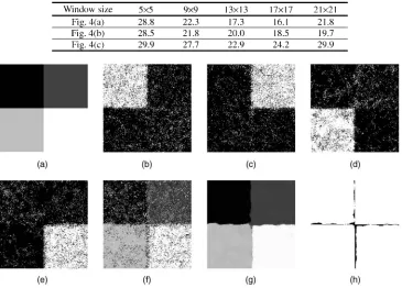
4.2 Multitexture Images

Fig. 4a shows a256256-sizetest image composed of four Brodatz textures. 2,000 training patterns (500 from each texture class) were used to train four SVMs. The best error rate obtained was 16.1 percent when using a 1717window (Table 7), while the average error rate of each one-against-others was 9.9 percent. It Fig. 6. Classification results for two texture classes: (a), (e), and (i) reference images, (b), (f), and (j) classification results for Figs. 3a, 3b, and 3c using only texture

classifier, (c), (g), and (k) postprocessed results of (b), (f), and (j), respectively, and (d), (h), and (l) misclassified pixels illustrated as black-gray levels.

TABLE 7

Error Rates (%) for Multitexture Images

arbitrated classification image. Fig. 7 shows the classification results. To understand the relevance of the results obtained with the proposed multiclass extension method for SVMs, a comparison was made of the classification results obtained from several different extension methods, including simple one-against-others, one-against-others with linear normalization [24], one-against-one, and all-at-once. For the all-at-once method, the implementation of a library for support vector machines (LIBSVM) made by Hsu and Lin [27] was utilized. Table 8 summarizes the results. Scaling with a neural network significantly improved one-against-others, which ranked as the best, meanwhile linear normalization and one-against-one came in second and third, respectively, and all-at-once showed a rather inferior performance.

Fig. 4b shows a256256-sizetest image composed of 5 VisTex textures. To train the classifier, 500 patterns were randomly selected from each texture class. The best error rate was 18.5 percent when using a1717window (Table 7). Fig. 4c shows another textured image consisting of nine VisTex textures. The image size is384384 and the size of each textured subregion is 128128. A total of 3,600 patterns were randomly selected (400 patterns from each texture class) as the training set, corresponding to about 2.4 percent of the total input patterns. The best error rate was 22.9 percent, obtained when using a1313window. In Fig. 4b, most of the errors were related to classifying the first texture class (Fabric.0007) due to difficulties in discriminating between the first and third texture classes (Fabric.0007 and Leaves.0003). In contrast, in Fig. 4c, many of the misclassified pixels were near the boundaries between the

(64=pffiffiffi2,32=pffiffiffi2,16=pffiffiffi2, and8=pffiffiffi2cycles per image), as described in [10]. The classification of the extracted features was performed using SVMs with a polynomial kernel of degree 5. To make the comparison fair, the feature images were not averaged before being fed to the classifier. In addition, for benchmark comparisons with other classification methods, experiments were also performed using neural networks. The networks included two hidden layers of size 20 with tangent hyperbolic activation functions and were trained using a back-propagation algorithm minimizing the mean squared error. Following the studies of Jain and Karu [12], where neural networks were also used to classify textures, the number of training steps was fixed at 1,000,000. To avoid local minima, the reported results were obtained by training 10 neural networks with different initial weights, and then selecting the minimal error over all the results.

Table 9 shows the results for the classification of Figs. 3a and 3b. For comparison, the results obtained from the SVM are also presented. With Gabor filters, a slight improvement was observed in Fig. 3a, while a significant increment in the error rate was observed in Fig. 3b. As such, the ability to achieve acceptable results without the use of Gabor filters indicates the possibility of using SVMs directly on texture patterns. In contrast, the better performance of the SVM over the neural network suggests that the decision boundary generated by the SVM was more effective in generalizing the given set of texture patterns.

5

C

This paper described an SVM-based texture classification method to assess the potential of SVMs in texture classification. With the exception of adopting the input configuration from the AR features, the proposed method does not use any external feature extraction scheme. Instead, the SVMs receive the gray-level values of the raw pixels as the input pattern. The rationale for this configuration is that an SVM has the capability of learning in high-dimensional spaces, such as gray-level texture pattern spaces, plus it can incorporate a feature extraction scheme within its own architecture. The validity of using polynomial kernels for texture feature extraction was also discussed from two feature extraction perspectives. The excellent performance achieved by an SVM when using these kernels also supported these views. For a multitexture classification problem, one-against-others decomposition is adopted and a neural network used to arbitrate the outputs of each SVM.

Future studies will investigate incorporating more texture-specific knowledge within SVM architectures. Possible choices include the selection of a feature space induced by specific kernels. For example, a Fourier-domain analysis would be helpful in extracting specific frequency and orientation components. Some of the main applications of this method include page-layout segmen-tation, text location in a video image, and textured object detection. Accordingly, further experiments are required related to real-world applications along with the fine-tuning of certain parameters, such as the input window size and structure of the arbitrator.

R

[1] H. Greenspan, R. Godman, R. Chellappa, and C.H. Anderson, “Learning Texture-Discrimination Rules in a Multiresolution System,”IEEE Trans. Pattern Analysis Machine Intelligence,vol. 16, no. 9, pp. 894-901, Sept. 1994.

[2] A.K. Muhamad and F. Deravi, “Neural Networks for the Classification of Image Texture,”Eng. Applications of Artificial Intelligence,vol. 7, pp. 381-393, 1994.

[3] Y.Q. Chen, M.S. Nixon, and D.W. Thomas, “On Texture Classification,” Int’l J. Systems Science,vol. 28, no. 7, pp. 669-682, 1997.

[4] M. Tuceryan and A.K. Jain, “Texture Analysis,” Handbook Pattern Recognition and Computer Vision, C.H. Chen, L.F. Pau, and P.S.P. Wang, eds., Singapore: World Scientific, pp. 235-276, 1993.

[5] R. Haralick, K. Shangmugam, and L. Dinstein, “Textural Features for Image Classification,”IEEE Trans. Systems, Man, and Cybernetics,vol. 3, pp. 610-621, 1973.

[6] P. Diaconis and D. Freedman, “On the Statistics of Vision: The Julesz Conjecture,”J. Math. Psychology,vol. 24, 1981.

[7] S.Z. Li, Markov Random Field Modeling in Computer Vision. New York: Springer-Verlag, 1995.

[8] H.J. Kim, E.Y. Kim, J.W. Kim, and S.H. Park, “MRF Model Based Image Segmentation Using Hierarchical Distributed Genetic Algorithm,” IEE Electronics Letters,vol. 34, no. 25, pp. 1394-1395, 1998.

[9] T. Randen and J.H. Husoy, “Filtering for Texture Classification: A Comparative Study,” IEEE Trans. Pattern Analysis Machine Intelligence, vol. 21, no. 4, pp. 291-310, 1999.

[10] A.K. Jain and F. Farrokhnia, “Unsupervised Texture Segmentation Using Gabor Filters,”Pattern Recognition,vol. 24, no. 12, pp. 1167-1186, 1991.

[11] C.S. Lu, P.C. Chung, and C.F. Chen, “Unsupervised Texture Segmentation via Wavelet Transform,”Pattern Recognition, vol. 30, no. 5, pp. 729-742, 1997.

[12] A.K. Jain and K. Karu, “Learning Texture Discrimination Masks,”IEEE Trans. Pattern Analysis Machine Intelligence,vol. 18, no. 2, pp. 195-205, Feb. 1996.

[13] V. Vapnik,The Nature of Statistical Learning Theory.New York: Springer-Verlag, 1995.

[14] B. Scho¨lkopf, K. Sung, C.J.C. Burges, F. Girosi, P. Niyogi, T. Pogio, and V. Vapnik, “Comparing Support Vector Machines with Gaussian Kernels to Radial Basis Function Classifiers,”IEEE Trans. Signal Processing,vol. 45, no. 11, pp. 2758-2765, 1997.

[15] S. Haykin,Neural Network—A Comprehensive Foundation,second ed. Prentice Hall, 1999.

[16] C.J.C. Burges, “A Tutorial on Support Vector Machines for Pattern Recognition,”Data Mining and Knowledge Discovery,vol. 2, no. 2, pp. 1-47, 1998.

[17] T.M. Cover, “Geometrical and Statistical Properties of Systems of Linear Inequalities with Applications in Pattern Recognition,” IEEE Trans. Electronic Computers,vol. 14, pp. 326-334, 1965.

[18] K.I. Laws, “Textured Image Segmentation,” PhD thesis, Univ. of Southern Calif., 1980.

[19] D.F. Dunn, W.E. Higgins, and J. Wakeley, “Determining Gabor Filter Parameters for Texture Segmentation,”Proc. SPIE Intelligence Robots and Computer Vision XI,pp. 51-63, 1992.

[20] S.C. Zhu, Y. Wu, and D. Mumford, “Filters, Random Fields and Maximum Entropy (FRAME)—Towards a Unified Theory for Texture Modeling,”Int’l J. Computer Vision,vol. 27, no. 2, 1998.

[21] B. Scho¨lkopf, C. Burges, and V. Vapnik, “Extracting Support Data for a Given Task,”Proc. Int’l Conf. Knowledge Discovery & Data Mining,pp. 252-257, 1995.

[22] B. Scho¨lkopf, “Support Vector Learning,” PhD thesis, Munich: Oldenbourg Verlag, 1997.

[23] J.-L. Chen and A. Kundu, “Unsupervised Texture Segmentation Using Multichannel Decomposition and Hidden Markov Models,”IEEE Trans. Image Processing,vol. 4, no. 5, pp. 603-619, 1995.

[24] E. Mayoraz and E. Alpaydin, “Support Vector Machines for Multi-Class Classification,” Technical Report IDIAP-PR 98-06, Dalle Molle Inst. for Perceptual Artificial Intelligence, 1998.

[25] P. Brodatz,Textures: A Photographic Album for Artists and Designers.New York: Dover, 1966.

[26] MIT Vision and Modeling Group.1998.

[27] C.-W. Hsu and C.-J. Lin, “A Comparison on Methods for Multi-Class Support Vector Machines,” technical report, Dept. of Computer Science and Information Eng., Nat’l Taiwan Univ., 2001.

[28] K.I. Laws, “Rapid Texture Identification,”Proc. SPIE Conf. Image Processing for Missile Guidance,pp. 376-380, 1980.

[29] J. Mercer, “Functions of Positive and Negative Type, and Their Connection with the Theory of Integral Equations,”Trans. London Philosophical Soc. (A), vol. 209, pp. 415-446, 1909.

[30] A.L. Yuille, J. Coughlan, S.C. Zhu, and Y. Wu, “Order Parameters for Minimax Entropy Distributions: When Does High Level Knowledge Help?”Proc. IEEE Conf. Computer Vision and Pattern Recognition,pp. 558-565, 2000.

.For more information on this or any other computing topic, please visit our Digital Library athttp://computer.org/publications/dlib.

TABLE 9