Abstract— A simulation study is executed with respect to an end-of-period discount for daily perishable products. In case that supplied products will not be sold out by end-of-period, the sales floor manager sometimes sells the products in a discount price in order to increase the revenue of the period. The reference price of consumers for the products is consequently declined and some consumers would not purchase the products at a regular sales price. It is important for the manager to take the reference price effect into account so as to improve long-term profit. This paper formulates the end-of-period discount problem within a framework of dynamic programming. Optimal pricings are derived in a simulation study to estimate the influence of inventory distribution on the optimal pricings.
Index Terms— dynamic programming, inventory control, optimal pricing, reference price effect, simulation.
I. INTRODUCTION
Packages of fresh prepared foods, such as sushi and sliced raw fish, are sold in retail stores nowadays in more countries. In case that the life of products only lasts one day due to deterioration of freshness, firms prepare appropriate amount of package products before opening with predicting the demand of the day, and sell them just for the day. Unsold products are to be disposed or reused as ingredients for other products. The firms hope to reduce the number of unsold products from both economical and ecological standpoints. On the days when the firms overestimate the demand, they sometimes discount the sales price of products or distribute coupons in order to stimulate consumer spending.
Such actions can improve profit of the day; they increase the revenue and decrease disposal cost. At the same time, however, the actions drop consumers' reference prices with which consumers judge if a sale price is a gain or a loss for them. The declined reference price reduces the future demand for the products sold at a regular price, which is called the reference price effect on demand, and it might decrease revenue in the long run. From a long-term business perspective, firms should discount sales prices advisedly.
Manuscript received April 22, 2010. This work was supported in part by Grant-in-Aid for Scientific Research(C), 2010, No.22510147.
Takeshi Koide is with Department of Intelligence and Informatics, Konan University, Kobe 658-8501, Japan (corresponding author, e-mail: [email protected]).
Hiroaki Sandoh is with Department of Management Science and Business Administration, Graduate School of Economics, Osaka University, Toyonaka 560-0043, Japan (e-mail: [email protected])
The reference price is well-known as the reference point in the prospect theory proposed by Kahneman and Tversky [1]. There are some researches studying promotional planning problems with the reference price effect to derive optimal pricing policies to maximize long-term revenues [2, 3, 4]. They targeted frequently purchased commodities and implicitly assumed that the firm could procure enough products to satisfy demands. In their models, the discount aims to stimulate demand and not to decrease the disposals of unsold products. The inventory quantity of the products is neglected in their models.
This paper discusses a discount pricing policy on daily perishable products considering reference price effects and inventory quantity. A firm can sell the products in a discount price just before the end of closing time to avoid the disposal of unsold products after the closing time. The firm determines an optimal sales price with considering inventory quantity, the demand for the products in the left business hours, and the deterioration of consumers’ reference price for long-term profit. The most essential factor in this study is taking inventory quantity into account in the model compared to models in past literature [2, 3, 4]. A mathematical model for the problem is formulated to derive an optimal pricing to maximize long-term profit. The optimal pricing is computed by a dynamic programming framework. The optimal pricing policies are discussed through simulation study for some long-term inventory distributions pattern. The simulation study reveals that the inventory distribution performs a crucial function in the optimal pricings and should not be neglected.
II. BACKGROUNDS AND SETTINGS A. Single Period Model
Consider a price-setting firm which deals in a single type of perishable products. The firm cannot be sold the unsold products in the following periods. The firm determines the sales price p and the inventory level q to maximize the expected profit on a single period. The optimums p* and q*
can be solved within a framework of the famous newsvendor problem [5].
Let D(p) = 0 – 1p + be the stochastic demand
function with respect to p, where 0 , 1 > 0 and is a random
variable with mean 0. When it holds D(p)q, the q – D(p) products are unsold and be disposed or reused at the unit cost
h, where h means the disposal cost if h > 0, and the salvage cost if h < 0. On the other hand, if D(p) > q, the D(p) – q
Simulation Study of Optimal Pricing
on Daily Perishable Products
with Reference Price Effect
demands are not satisfied and estimated a penalty at the per-unit cost s > 0. Let c be the unit procurement cost of the products.
Introducing z = q – E[D(p)], so-called stocking factor, the optimal price p* which maximizes the expected profit
E[(p, z)] is given by the following equation [5]:
1 0 *
2 ) (
z p
p , (1)
where (z) is the expected amounts of shortages and p0 is the optimal price which maximizes the riskless expected profit
E[(p – c)D(p)]. From (1), the optimum p* only depends on z.
With letting p = p*(z), the expected profit E[(p*(z), z)] becomes just a function with respect to z, then the optimal stocking factor z* is derived, then so are p* and q* [5].
B. Multi-Period Model with Reference Price Effect
Here, we target a finite horizon model over T multiple periods; period t = 1, 2, …, T. Similarly to the previous model, unsold products at the end of period cannot be left over the following periods. With the reference price effect, even under such a setting, the optimal prices for multiple periods are not equal to the price given by (1).
The demand function comprising the reference price effects is modeled as follows:
D(p, r) = 0 – 1p + 2[r – p]+ – 3[p – r]+, (2)
where 2, 3 > 0 and [x]+ = max(x, 0). Consumers perceive a
sold product as a gain if the sales price p is less than their reference prices r, and the demand increases by 2(r – p) from
the fundamental demand D(p). If the sales price p is above the reference price r, the demand decreases by 3(p – r). When it
holds 2 < 3, 2 = 3, and 2 > 3, the consumers are
respectively referred as to loss-averse, loss-neutral, and loss-seeking [1].
The consumers update their reference prices depending on the sales price. It is assumed that the reference price rt on period t + 1 is determined by the reference price rt and the sales price pt on the previous period:
rt + 1 = rt + (1 – ) pt. (3) The exponential smoothing represented by (3) is the
most commonly adopted in the literature [2, 3, 4]. The smoothing parameter implies how strongly the reference price is affected by past prices, where 01 . The consumers with lower have a short-term memory, and they are strongly influenced by recent sales prices.
In this case, the objective is to find the optimal prices {p1*, p2*, …, pT*} and the optimal inventory levels {q1*, q2*,
…, qT*} to maximize the current value of the profit over T periods. The problem is more complex than that in a single period case even though D(p, r) is deterministic as shown in (2). It can be generally solved within a dynamic programming framework.
C. Promotion Planning Problems
The past studies with considering reference price [2, 3, 4] are aimed to promotion planning problems, where a firm sometimes sells the target products at discount prices as a promotion to maximize a long-term profit. They assume that their target products are frequently purchased commodities and their supply is abundance. As the result, they consider
neither the possibility of out of stock nor that of disposal due to the expiration of the products. The profit in their studies is simply
(p, r) = pD(p, r). (4)
Popescu and Wu [4] have derived some qualitative results regarding the optimal pricing trajectory for the promotion planning problem. Their most important result is that the optimal pricing path converges to a unique constant price, which can be obtained from a closed-form equation, if consumers are loss neutral or loss aversion. The closed-form equation cannot be applied to our problem which considers the inventory quantity.
III. TARGET PROBLEM A. Problem Descriptions
In this study, we treat a single type of products over T
multiple periods. Each period is divided into two terms: term 1 and term 2. Term 2 and term 1 represent the end-of-period and the other, respectively. The firm starts to sell the product at the beginning of term 1 at the regular price pH. Let qt be the left stocking quantity at the beginning of term 2 in period t. In general, the inventory quantity qt varies stochastically because of the deviation between the predicted and observed demands in term 1, and we consider several cases regarding the inventory distribution {qt} in the next section.
At the beginning of term 2, the floor sales manager determines the sales price pt within an available price range
p= [pL, pH]. Assume D(p,r) is given by (2) in common over
T periods and nonnegative for any p and r within p. The objective in this study is to derive an optimal price {p1*, p2*, …, pT*} in term 2 to maximize the present value of total profit over T periods, with considering the forecasted inventory distribution {q1, q2, …, qT} and the demand D(p, r) in term 2. Note that {q1, q2, …, qT} are not design variables but given in this study. Furthermore, the determination of the regular price pH and the initial inventory level at the beginning of term 1 is excluded from this model, unlike the single period model in the previous section.
Consumers are assumed to be homogeneous and have a common reference price rt in period t. It is postulate that consumers are segmented by their visiting terms: within term 1 and term 2. The assumption means that the pricing in term 2 does not affect the consumers in term 1.
B. Formulation
Suppose that there are q unsold products at the beginning of term 2 in a certain period. If the products are sold at price p
in term 2 for consumers with reference price r, the firm sells min[D(p, r), q] products, disposes [q – D(p, r)]+ products, and loses [D(p, r) – q]+ consumers. The profit (p, q, r) in term 2 in the period is given by
(p, q, r) = min[D(p, r), q]p – cq
– h [q – D(p, r)]+ – s[D(p, r) – q]+ (5) Let r1 be the consumers’ reference price on period 1, the
Problem M:
T
t
t t t t
p p q r
r V
p
t 1
1 1
1
1 q, max , , , (6)
subject to (3) for t = 1, 2, …, T – 1. The value function
V1(q1, r1) implies the maximum present value over T periods
with inventories q1 = {q1, q2, …, qT} and initial reference price r1.
Problem M can be transformed as follows and its solution is derived by dynamic programming.
t
t t t
p t t
t r W p q r
V
p t
, , max ,
q , (7)
Wt(pt, qt, rt) = (pt, qt, rt) + V(qt+1, rt + (1 – )pt), (8)
VT(· ,·) = 0, (9)
where qt = {qt, qt+1, …, qT}, t = 1, 2, …, T. The value of the reference price rt in Vt(qt, rt) is discretized in price range p to execute the dynamic programming since the value of rt is a real number.
Define optimal pricing pt* and the corresponding reference price rt* by the following equations:
t
t t t
pt t t
t p r W p r
p
p t
, , max arg ,
*
* q q
, (10)
rt* = rt–1* + (1 – ) pt–1*, (11)
r1* = r1. (12)
To avoid the ambiguity of multiple solutions, arg maxxf(x) refers to the largest value of x which maximizes the function f. The vector {p1*, p2*, ..., pT*} is named optimal pricing path.
IV. SIMULATION STUDIES A. Simulation Settings
This section discusses the optimal pricing policy through the computed optimums in simulation study under several inventory distributions. Three types of so-called “optimal” pricings are compared in this section. The first is the exact optimal pricing pt*, obtained by (10). The second is a myopic optimal pricing ptM* and the last is the single period maximizing pricing p~t.
The myopic optimal pricing ptM* is the optimal pricing for Problem M with T = 1 and is obtained by
t t
p t t M
t q r p q r
p
p
, , max arg ,
*
. (13) The myopic optimal pricing takes the reference price effect
into account, but ignores the influence of the determined price ptM* on the reference prices rt+1 in the future.
The single period maximizing pricing p~t does not consider even the reference price effect and is computed by
q
p q p
p t
p t t
p
, , max arg
~
. (14) The single period maximizing pricing depends only on the
inventory qt and becomes constant for any t for a constant qt. The demand in this experiment has the following fashion:
D(p, r) = 0 – 1p + 2[r – p]+ / r – 3[p – r]+ / r. (15)
The reference price effect in (15) signifies a relative difference perception, motivated by the Weber-Fechner law
in psychophysics. According to some experiments with respect to the prospect theory [6], the consumers are assumed to be loss aversion. Concretely, we set the parameters 2 = 75
and 3 = 150. The regular price pH of the products is 500 and the minimum available price pL is 200. The initial reference price r1 is assumed to be equal to the regular price, 500. The
other parameters are set as follows: 0 = 100, 1 = 0.1,
= 0.95, c = 300, h = 50, and s = 0.
The exact optimal price pt* and its competitors ptM* and t
p
~ are computed in terms of 0.5.
B. Case 1: Constant Inventories
This subsection discusses the optimal pricings under the situation where inventories {qt} are constant for any t. The firm should sell the products at the regular price pH when it holds qt D(pH,pH)50. We hence consider the cases qt is constantly equal to 55, 60, 65, and 70. The parameter T is set to 100 or 150 so that the optimal prices substantially converge to constant values.
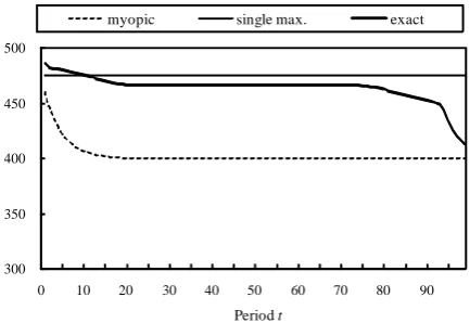
The trajectories of the three types of optimums are illustrated in Fig. 1 where qt = 60, = 0.4, and T = 100. The myopic price ptM* decreases monotonously, then converges to a constant price 400. The single period maximizing price p~t has a constant value 475 since it depends on the constant qt alone. The exact optimal price exhibits analogous behavior to the myopic price till t = 70, namely decreases and converges to a certain level pt* = 467, then decreases till the end of planning periods t = 100. The downward price is occurred due to the limitation of the planning period. A discount price has less influence on future profit toward the end of the planning periods. The firm therefore should reduce the sales price to emphasize short-term profit.
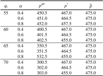
Owing to the discount factor , if the length of planning periods T is sufficiently great, the final periods can be ignored. We hence focus on the temporary convergence value before the final periods, denoted by p*. Let pM* and p~ be the convergence value of the myopic pricing and the constant single period maximizing pricing. Table 1 summarizes the three types of prices in several settings of qt and . For all cases in Table 1, it holds
pM* p* ~p. (16)
Equation (16) can be interpreted as follows. The myopic policy settles a low price to stimulate demand since it neglects the disadvantage caused by declined consumer’s
300 350 400 450 500
0 10 20 30 40 50 60 70 80 90
Period t
[image:3.595.315.532.56.205.2]myopic single max. exact
reference price. The single period maximizing policy sets a high price without taking reference effect on demand into account. Popescu and Wu [4] proved that (16) holds in their model where inventory quantity is ignored. Since our model is an extension of theirs, we expect (16) also holds in our model.
Table 2 represents the ratios of V1(q1, r1) in (6), the
current value of total profit, by the three types of optimal pricings, where V*, VM*, and V~are respectively V1(q1, r1) by
the exact optimal pricing, by the myopic pricings, and by the one-day profit-maximizing pricings. The current values VM*
and V~relatively deteriorate when the constant inventory level qt increases. It is noticeable that the myopic pricings lost a profound profit by the discarded discounts in case of grater
.
C. Case 2: Periodic Inventories
This subsection discusses the optimal pricings under the situation where inventory quantity yt varies periodically. Here, we consider the cases where the length of inventory cycle is 2, such as qt = qL, qH, qL, qH, … (qL < qH), and the average between qL and qH is equal to D(pH, pH) = 50. Figure 2 and Figure 3 illustrate the fluctuation of the optimal pricings in the cases where (qL, qH) = (40, 60) and (qL, qH) = (30, 70), respectively, = 0.4, and T = 100. The optimal pricings synchronize according to the periodic variation of qt. The single period maximizing pricing p~t is identical to that in Case 1 for the same value of qt; p~t = 475 if qt = qH (=60, 70) and ~pt = 500 otherwise. On the other hand, pt* and
ptM* do not correspond with those in Case 1. Analogous to the previous subsection, let p* and pM* be respectively the convergence prices of pt* and ptM* for qt = qL and qt = qH. Additionally, let r* and rM* be the reference prices according to p* and pM*, respectively. Tables 3 and 4 compare the above
400 420 440 460 480 500
0 5 10 15 20
Period t
[image:4.595.75.255.69.202.2]myopic single max. exact
Figure 2. Optimal prices in Case 2 (qL = 40, qH = 60, = 0.4).
400 420 440 460 480 500
0 5 10 15 20
Period t
myopt single max. exact
[image:4.595.322.534.208.331.2]Figure 3. Optimal prices in Case 2 (qL = 30, qH = 70, = 0.4).
Table 3. Exact Optimum p* in Case 1 and Case 2.
Case 1 Case 2
qt 40 60 40 60
p* 500.0 467.0 499.0 454.5
r* 500.0 467.0 467.5 486.5
D(p*, r*) 50.0 53.3 40.0 59.5
(p*, q
t, r*) 8,000 6,556 7,956 9,009
Case 1 Case 2
qt 30 70 30 70
p* 500.0 467.0 500.0 417.0
r* 500.0 467.0 441.0 476.5
D(p*, r*) 50.0 53.3 29.9 67.7
(p*, q
[image:4.595.96.237.232.364.2]t, r*) 6,000 6,556 5,963 7,100
Table 4. Myopic Optimum pM* in Case 1 and Case 2.
Case 1 Case 2
qt 40 60 40 60
pM* 500.0 400.5 499.0 454.5
rM* 500.0 400.5 467.5 486.5
D(pM*, rM*) 50.0 60.0 40.0 59.5
(pM*, q
t, rM*) 8,000 6,008 7,956 9,009
Case 1 Case 2
qt 30 70 30 70
pM* 500.0 300.5 485.0 400.0
rM* 500.0 300.5 424.5 461.0
D(pM*, rM*) 50.0 70.0 30.1 69.9
(pM*, q
t, rM*) 6,000 18 5,550 6,966
Table 1. Convergence Prices in Case 1.
qt pM* p* p~
55 0.4 450.5 467.0 475.0
0.6 451.0 464.5 475.0 0.8 452.0 457.5 475.0
60 0.4 400.5 467.0 475.0
0.6 401.5 464.5 475.0 0.8 402.5 455.0 475.0
65 0.4 350.5 467.0 475.0
0.6 351.5 464.5 475.0 0.8 532.5 455.0 475.0
70 0.4 300.5 467.0 475.0
0.6 302.0 464.5 475.0 0.8 303.0 455.0 475.0
Table 2. Ratios between Optimal Profits in Case 1.
qt VM* / V* V~/ V* 55 0.4 99.55% 99.51%
0.6 99.67% 99.42% 0.8 98.64% 98.78% 60 0.4 93.78% 99.19%
0.6 94.85% 98.91% 0.8 96.85% 97.55% 65 0.4 74.73% 98.61%
0.6 78.16% 98.12% 0.8 85.22% 95.96% 70 0.4 20.82% 97.55%
[image:4.595.331.524.380.557.2] [image:4.595.331.523.584.760.2]values and the corresponding demands and profits in Case 1 and Case 2.
Table 3 shows that the exact optimal price p* in Case 2 is smaller than that in Case 1. In the case of qt = 70, for instance,
p* = 467 in Case 1 and p* = 417 in Case 2. The inventory quantity is 70 for every period in Case 1, whereas it falls down to 30 the next period in Case 2. The firm can sell products at a high price in the period with qt = 30, and consequently consumers’ reference price is elevated. The firm can sell products at a lower price to stimulate demands in the period with qt = 70 in Case 2 for consumers with higher reference price compared with those in Case 1.
Table 4 reveals that the myopic optimums pM* in Case 2 have smaller fluctuation than in Case 1. For example, the myopic optimums are 500.0 and 300.5 in the cases of qt = 30 and qt = 70 in Case 1, respectively. When (qL, qH) = (30, 70) in Case 2, pM* = 485.0 and pM* = 400.0. Since the myopic pricing only optimizes the sales price of the period with considering consumers’ reference price, the myopic optimum in Case 2 is inevitably higher on the period with qL than that in Case 1 with a constant qL, and lower on the period with qH than that in Case 1 with a constant qH.
As shown in Table 2 for Case 1, we have estimated the ratio of the current value of total profits by the three types of optimal pricings in Case 2, which are summarized in Table 5. The current values by both the myopic policy and single period maximizing policy are deteriorated when the difference of inventory fluctuation, namely qH – qL, increases. It is also noticeable that the myopic policy is an appropriate approximation of the exact policy for the situation with small fluctuation of inventory level and with a great .
D. Case 3: Normal Distributed Inventories
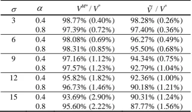
This subsection discusses the optimal pricings under the situation where inventories qt follows a normal distribution with mean D(pH, pH) = 50. The standard deviation of the distribution has five levels 3, 6, 9, 12, and 15. A thousand of inventory patterns are randomly generated for each . The
length of planning period T is set to 100. The three types of optimal prices and their corresponding values of the objective function are computed for the generated inventory patterns.
Table 6 indicates the results of experiments. The values outside and insides the brackets represents the mean and the standard deviation for 1,000 patterns. Both V~ / V* and
VM* / V* decrease as increases. Note that VM* / V* in Case 3 with = 3 are less than that in Case 2 with (qL, qH) = (40, 60), whose standard deviation is 10 . The result means that irregularity of inventory levels reduces the precision of the approximate optimum computed by the myopic pricing policy.
V. CONCLUSIONS
This paper has proposed a mathematical model for an optimal end-of-period discount pricing on perishable products without leftover. The proposed model incorporates not only the reference price effect but also the amount of inventory. The optimal pricing has been derived through dynamic programming and numerical experiments revealed that the optimal pricing substantially depends on the inventory distribution. For the loss-averse consumers, the firm should sell the products at a constant price when the forecasted inventories in the future are also constant. When the future inventories cycle periodically, the firm should vary the sales price periodically according to the fluctuation of inventory. The myopic price deteriorates compared with the exact optimum in case that inventory quantity varies randomly. The exact optimum is required for realistic uncertain situations.
An algorithm to derive the exact optimum has to be improved in order to execute in shorter time for larger size of problems. Theoretical analyses with respect to the optimum are also necessary to find more general insights on the optimal pricings. The models with another manner to update consumer's reference price is attractive to research. Fredrickson and Kahneman mentioned that consumers tend to memorize the lower price strongly than higher price [7], which seems to be more practical. The optimal pricing with such an update mechanism will be discussed in forthcoming papers.
REFERENCES
[1] D. Kahneman and A. Tversky, “Prospect theory: An analysis of decision under risk,” Econometrica, vol. 47, 1979, pp. 263–291. [2] E. A. Greenleaf, “The impact of reference price effects on the
profitability of price promotions,” Marketing Science, vol. 14, 1995, pp. 82–104.
[3] P. K. Kopalle, A. G. Rao, and J. L. Assuncao, “Asymmetric reference price effects and dynamic pricing policies,” Marketing Science, vol. 15, 1996, pp. 60–85.
[4] I. Popescu and Y. Wu, “Dynamic pricing strategies with reference effects,” Operations Research, vol. 55, 2007, pp. 413–429.
[5] N. C. Petruzzi and M. Dada, “Pricing and the newsvendor problem: A review with extensions,” Operations Research, vol. 47, 1999, pp. 183–194.
[6] G. Kalyanaram and R. S. Winer, “Empirical generalizations from reference price and asymmetric price response research,” Marketing Science, vol. 14, pp. G161-G169, 1995.
[image:5.595.76.259.72.186.2][7] B. L. Fredrickson and D. Kahneman, “Duration neglect in retrospective evaluations of affective episodes,” Journal of Personality and Social Psychology, vol. 65, pp. 45–55, 1993.
Table 5. Ratios of Optimal Values in Case 2.
qL qH VM* / V* V~/ V*
40 60 0.4 99.16% 94.25%
0.8 100.00% 93.30%
35 65 0.4 98.19% 87.48%
0.8 99.99% 86.81%
30 70 0.4 96.59% 80.23%
0.8 99.99% 79.53%
25 75 0.4 92.82% 71.11%
0.8 99.65% 71.05%
20 80 0.4 85.87% 58.45%
[image:5.595.70.264.214.327.2]0.8 98.60% 59.06%
Table 6. Ratios of Optimal Values in Case 3.
VM* / V*
V~/ V* 3 0.4 98.77% (0.40%) 98.28% (0.26%)