An Efficient Implementation of an Active Set Method for SVMs
Katya Scheinberg [email protected]
Mathematical Science Department IBM T. J. Watson Research Center 1101 Kitchawan Road
Yorktown Heights, NY
Editors: Kristin P. Bennett and Emilio Parrado-Hern´andez
Abstract
We propose an active set algorithm to solve the convex quadratic programming (QP) problem which is the core of the support vector machine (SVM) training. The underlying method is not new and is based on the extensive practice of the Simplex method and its variants for convex quadratic prob-lems. However, its application to large-scale SVM problems is new. Until recently the traditional active set methods were considered impractical for large SVM problems. By adapting the methods to the special structure of SVM problems we were able to produce an efficient implementation. We conduct an extensive study of the behavior of our method and its variations on SVM problems. We present computational results comparing our method with Joachims’ SVMlight(see Joachims,
1999). The results show that our method has overall better performance on many SVM problems. It seems to have a particularly strong advantage on more difficult problems. In addition this al-gorithm has better theoretical properties and it naturally extends to the incremental mode. Since the proposed method solves the standard SVM formulation, as does SVMlight, the generalization properties of these two approaches are identical and we do not discuss them in the paper.
Keywords: active set methods, support vector machines, quadratic programming
1. Introduction
In this paper we introduce an active set method to solve the following convex quadratic program-ming (QP) optimization problem which is defined by the classic soft margin SVM formulation (see, for example, Cristianini and Shawe-Taylor, 2000).
max −1
2α T
Qα−cTξ
−Qα+by+s−ξ=−e, (1)
0≤α≤c, s≥0, ξ≥0,
where α ∈Rn is the vector of the dual variables, b is the bias (scalar) and s and ξ are the n-dimensional vectors of the slack and the surplus variables, respectively. y is a vector of the labels,
±1. Q is the label encoded kernel matrix, Qi j =yiyjK(xi,xj), e is the vector of all 1’s of length n and c is the penalty vector associated with the errors (in standard soft margin SVMs the vector c is a product of vector e and a scalar penalty C, but here we will allow for any nonnegative vector c). The dual of this problem is
min 1 2α
T
s.t. yTα=0, (2)
0≤α≤c.
To confirm that problem (1) is equivalent to the traditional soft margin SVM formulation
min 1 2w
T
w+cTξ
s.t. yi(wTxi−b)−si+ξi≥1, i=1, . . . ,n (3)
s≥0, ξ≥0,
observe that (2) is the same as the dual of (3) and from optimality conditions of (3) and (2) we have w=∑ni=1yiαixi. Substituting this expression for w to (3) and denoting Qi j=yiyjαiαjx
T ixj (or Qi j=yiyjαiαjK(xi,xj)in the kernel case) we obtain the convex QP formulation (1), which we will consider in this paper. Hence, (1) and soft margin SVM enjoy thesame generalization properties.
General convex QPs are typically solved by one of the two approaches: interior point method approach oractive set method approach. If the Hessian of an objective function (matrix Q in the case of SVM) and/or the constraint matrix of the QP problem is large and sparse then an interior point method is usually the method of choice. If the problem is of moderate size but the matrices are dense, then active set method is preferable. In SVM problems the Q matrix is typically dense. Thus, large SVM problems present a challenge for both approaches. It was shown by Fine and Scheinberg (2001) and Ferris and Munson (2000) that for some classes of SVMs, for which Q is dense but low-rank, one can adapt an interior point method to work very efficiently. However, if the rank of Q is high, an active set approach seems to remain the only main alternative.
One of the most “traditional” active set methods in the optimization literature is the Simplex method for linear programming (LP) problems. The Simplex method is known to have very good practical performance. The QP analogues, though not as extensively tested in practice, are also considered to be very efficient. There are a few methods based on the Simplex method idea for solving QP problems (see Fletcher, 1971; Goldfarb, 1972; Goldfarb and Idnani, 1983). Many of them are theoretically equivalent, meaning that they produce the same sequence of iterations, but they have different numerical properties (such as per-iteration complexity and numerical stability). In this paper we derive an implementation targeted to SVM problems based on the framework described in Fletcher (1971), Goldfarb (1972) and Nocedal and Wright (1999).
The main idea of this method in the context of SVM is to fix, at each iteration, all variables in the current dual active set1at their current values (0 or c), and then to solve the reduced dual problem. After obtaining a solution - decide whether it is optimal for the overall dual problem (same as being feasible for the overall primal problem), or if any of the dual variables should be released from the active set.
When applied to SVM, this approach poses the following problem: if the complement of the dual active set (the set of “free” variables) has large cardinality, then solving the restricted subprob-lems may be too expensive, since Q is completely dense. Also determining the next variable to leave the active set may be expensive for the same reason. Therefore, updating all “free” variables at once was considered impractical.
The most common approach to large SVM problems is to use a restricted active set method, such as chunking (Boser et al., 1992) or decomposition (Osuna et al., 1997; Joachims, 1999) where
at each iteration only a small number of variables are allowed to be varied. The size of such “chunk” is determined heuristically or is chosen by the user. There are a few skillfully implemented SVM solvers based on this type of restricted active set methods (Joachims, 1999; Platt, 1999). The main disadvantage of these methods is that they tend to have slow convergence when getting closer to the optimal solution. Moreover, their performance is sensitive to the changes in the chunk size and there is no good way of predicting a good choice for the size of the chunks for a particular problem.2
A full active set method, such as the one presented in this paper, avoids these disadvantages. The method itself is not new (see Nocedal and Wright, 1999). Our contribution is to adapt it to the SVM framework and provide an efficient implementation.
First we notice that a support vector that violates the margin constraint (that is the ξ surplus variable is positive) corresponds to a variableαwhich is at its upper bound and therefore is in the dual active set. The complement of the dual active set contains variablesαthat are strictly between the upper and lower bounds. Such variables correspond only to the support vectors that are exactly on the margin (that is both the corresponding slack and the surplus variables are zero). The current number of such support vectors, ns, is the size of the reduced QP (RQP). Solving such RQP directly (say, by an IPM method, as it is done in SVMlight) requires at least O(n3s)operations, which might be prohibitively expensive if repeated over and over again and if ns is relatively large. We do not solve RQP directly, but only make one step toward its solution at each iteration. Moreover, the active set is incremented only by one variable at a time (either one variable leaving, or one entering the active set), hence we can store and update a factorization of the reduced matrix Q. Each update takes O(n2s)operations and so does solving a system of equations with the reduced matrix Q.
At each such step toward the optimal solution of the RQP, we either find that solution or en-counter a bound on one of the “free” variables. In the latter case this variable is included into the active set and the process repeats.
This process does not always produce an optimal solution to the subproblem, but usually pro-duces a good approximation of it. Typically this does not affect the overall number of iterations significantly, whereas the reduction of the per-iteration cost is significant.
The RQP may sometimes have an infinite solution, if reduced matrix Q is singular. In this case an infinite descent direction is computed and a step is taken along this direction until one of the variable bounds is encountered. We provide the full treatment of the various cases for solving the RQP subproblem. We use the approach described in Frangioni (1996).
If the search for the optimum of the RQP subproblem is terminated then our method determines whether the primal feasibility was achieved and if not, which dual variable should leave the active set. To do that we need to compute a product of a submatrix of Q that corresponds to the variables at their upper bounds and the unit vector of an appropriate length. This can be very expensive to compute at each iteration, instead one should rather store and update the result of this multiplication. Another advantage of using “one-variable-at-a-time” increments is in potentially reducing the cost of such updates.
The multiple updates to the active set, which are used in “chunking” and “decomposition” meth-ods could still have an advantage if the overall number of iterations were significantly smaller than in the case of single updates. But as our computational results indicate this is not the case. We offer some intuition to support this claim. Assume that your data contains 10 identical data points which at the current iteration are the most violated examples and we would like to introduce them into the
next “chunk”. Introducing all 10 at once implies 10 times more work than introducing just one. Yet since they are identical, introducing just one produces the same result as introducing all ten. Since the training data is often somewhat repetitive (there may not be identical points, but rather very similar points, for instance, in clustered data sets) this example is not too far fetched.
As the computational results show, our method has particular advantage over SVMlighton prob-lems where the number of the support vectors or the number of outliers is large (but not necessarily excessive, such as∼1000 out of 20000 vectors). Our algorithm currently requires the storage of the Cholesky factors of the reduced matrix Q, which might require excessive amount of memory for problems where the number of unbounded support vectors is very large. However, this often means that the chosen kernel suffers from overfitting the data, so the problem is badly posed in some sense, unless the entire test set is very large, in which case one should consider a different implementation, and, possibly, a more powerful computer.
The most expensive step of our algorithm (and of SVMlight, in fact) is pricing the primal con-straints and choosing the next constraint to enter the active set. We will compare two approaches. One of these approaches isshrinking, which is used by SVMlight, and the other issprint which is an industry standard in advanced implementations of LP solvers (Bixby et al., 1992). We observe that sprint appears to work better than shrinking on difficult SVM problems.
The proposed method enjoys several theoretical advantages compared to the methods based on chunking. First of all it converges in a finite number of iterations (Fletcher, 1971; Frangioni, 1996). In the worst case this number might be exponential, but it is hardly the case in practice. The method is also well suited for analysis of various situations. For instance, in Balcazar et al. (2001) a randomized active set algorithm for SVM is introduced and shown to have a quasi-linear average complexity. Our algorithm can be easily adapted to fit the randomized framework of Balcazar et al. (2001), hence similar average case results apply.
Recently, active set methods for SVM similar to ours were used in Cauwenberghs and Poggio (2001) for incremental learning and in Hastie et al. (2004) for generating the entire regularization path. Their methods, unlike ours, require primal and dual feasibility to be satisfied at every iteration and progress by changing the optimization problem itself (in a manner dictated by the respective uses of their methods). However, many of the efficiency issues of the algorithms are similar, such as the possible singularity of the reduced matrix Q and efficient updates of its Cholesky factorization. Though we choose to focus on one specific active set method in this paper, we believe the the experience we present here will be useful for other active set methods for SVM problems. Some of the ideas presented in the paper to improve the efficiency of the active set methods for SVMs were also suggested in Kaufman (1998).
2. Dual Active Set Method for SVMs
Any optimal solution to problems (1) or (2) must satisfy the Karush-Kuhn-Tucker (KKT) necessary and sufficient optimality conditions:
1 αisi=0, i=1, . . . ,n
2 (ci−αi)ξi=0, i=1, . . . ,n
3 yTα=0,
4 −Qα+by+s−ξ=−e,
5 0≤α≤c,
6 s≥0,ξ≥0.
Let us introduce some notation. A primal-dual solution(α,b,s,ξ)is calleddual basic feasible if it satisfies condition 1-5 of the KKT system, but may violate condition 6. For a given dual basic feasible solution,(α,b,s,ξ), we partition the index set I={1, . . . ,n}into three sets I0, Ic and Isin the following way:∀i∈I0si≥0 andαi=0,∀i∈Icξi≥0 andαi=ciand∀i∈Issi=ξi=0 and 0<αi<ci. It is easy to see that I0∪Ic∪Is=I and I0∩Ic=Ic∩Is=I0∩Is= /0. We will refer to Is as theprimal active set and to I0∪Icas thedual active set. Let ns=|Is|, n0=|I0|and nc=|I0|,
Based on the partition(I0,Ic,Is) we define Qss (Qcs Qsc Qcc, Q0s, Q00) as the submatrix of Q whose columns are the columns of Q indexed by the set Is(Ic, Is, Ic, I0, I0) and whose rows are the rows of Q indexed by Is(Is, Ic, Ic, Is, I0). We also define ys(yc, y0) andαs(αc,α0) and the subvectors of y andαwhose entries are indexed by Is(Ic, I0). ccis the part of vector c indexed by Ic and by e we denote a vector of all ones whose size is determined by the context.
To initiate the algorithm we assume that we have a dual basic feasible solutionα0,b,s0,ξ0and
the corresponding partition(I00,Ic0,Is0). For example settingα0=0 and I0={1, . . . ,n}produces a starting point for the algorithm.
We know that∀i∈I0αi=0 and∀i∈Ic αi=ci. Then if we fix the variables in the dual active set then our dual problem reduces to
minαs 1 2α
T
sQssαs+c T
cQcsαs−e T
αs
s.t. y
T
sαs=−y T ccc, 0≤αs≤c.
The outline of the algorithm is the following:
Step 0 Givenα0,β0, s0,ξ0find initial Is, I0and Ic.
Step 1 If Is=/0, go to Step 2, otherwise:
(i) Solve
minαs
1 2α
T
sQssαs+c T
Qcsαs−e T
αs (4)
s.t. yTsαs=−y T ccc.
(ii) From the current iterate make a step along direction d until for some i∈Is αi =0 or αi=cior until solution is reached.αks+1is the new point.
(iii) If for some i∈Is,αki+1=0,
then update Is:=Is\{i}, I0:=I0∪ {i}, k :=k+1 and go to the beginning of Step 1. (iv) If for some i∈Is,αki+1=ci,
then update Is:=Is\{i}, Ic:=Ic∪ {i}, k :=k+1 and go to the beginning of Step 1.
(v) If the optimum is reached in step (ii); that isαks+1=α∗s, proceed to Step 2.
Step 2 Partition I0into I00 and I000and partition Icinto Ic0 and Ic00 (i) Compute s00, the subvector of s indexed by I00:
s00=−Q00sαks+1−y00β+1−Q00ccc andξ0c, the subvector ofξindexed by Ic0:
ξ0
c=Q0csαks+1+y0cβ−1+Q0cccc,
where Q00sand Q00c(Q0csand Q0cc) are the submatrices of Q0sand Q0c, respectively, (Qcs and Qcc, respectively ) with rows index by I00(Ic0).
(ii) Find i0=argmini{si: i∈I00}. Find ic=argmini{ξi: i∈Ic0}.
(iii) If si0 ≥0 andξic ≥0 then if I0
06=I
0 or Ic06=Icthen let I00:=I0 and Ic0:=Ic and go to Step 2(i). Else, the current solution is optimal, Exit.
If si0≤ξic, then Is:=Is∪ {i0}and I0:=I0\{i0}.
Else, Is:=Is∪ {ic}and Ic:=Ic\{ic}. k :=k+1, go to Step 1.
We will now discuss in details the implementation of the steps of the algorithm.
2.1 Solving the Quadratic Subproblem
When matrix Qss is strictly positive definite then problem (4) has a unique finite solution. This solution satisfies the KKT conditions:
−Qssαs+y T
sβ = −e T
+cTcQcsαs
yTsαs = −c T cyc,
or, in matrix form,
−Qss ys yTs 0
αs β
=
−e+Qsccc
−cTcyc
. (5)
Since we are considering the case when Qss is nonsingular, we can findβby taking the Schur complement of the above system
(yTsQ−ss1ys)β=y T
Consider the Cholesky factorization Qss=LsLs T
and denote Ls−1ysby r1and Ls−1(−e+c T cQcs) by r2. Then the solution to (5) is
β=r T 1r2−c
T cyc r1Tr1
, αs=L
−T
s (r1β−r2).
It is often the case, however, that Qss is not strictly positive definite. This can even occur when an RBF kernel (which is strictly positive definite for distinct data points) is used, if the set Iscontains indices of two identical data points with different labels.
If, due to singularity of Qss, system (5) is underdetermined, this means that problem (4) has an unbounded solution. In this case Step 1(i) should produce an infinite descent direction for (4). A direction d is an infinite direction if it satisfies Qssd=0 and y
T
sd=0. Depending on the sign of(−e+ceTQcs)
T
d either d or−d is chosen as the infinite descent direction. Variableβremains unchanged in this case. We use the approach for positive semidefinite QP problems described in Frangioni (1996) and Kiwiel (1989).
We consider several cases.
Case 1
Let Qss have only one zero eigenvalue. Then, subject to permutation and without loss of generality, its Cholesky factorization can be written as
Qss=
Ls 0 lsT 0
Ls T ls 0 0 ,
where Ls∈R(ns−1)×(ns−1)and Ls∈Rns−1. Then system (5) can be written as
−LsLs T
−Lsls y1:ns−1
−lsTLs T
−lsTls yns y1:ns−1 yns 0
α1:ns−1 αns β =
(−e+Qsccc)1:ns−1 (−e+Qsccc)ns
−cTcyc
,
where, following Matlab notation, y1:ns−1(α1:ns−1,(−e+Qsccc)1:ns−1) denote the first ns−1 elements of vector y (α,(−e+cQsce)) and yns (αns,(−e+Qsccc)ns) denotes the last compo-nent of this vector.
Let r1=Ls−1y1:ns−1 and r2=Ls−1(−e+Qsccc)1:ns−1. By expressing α1:ns−1 in the above system throughαns andβ, and by consecutively eliminatingαns we obtain
(−lsTr1+yns)β= (−e+Qsccc)ns−l T sr2. We now have two cases.
(a) If lsTr16=yns then system (5) still has a unique solution β = (−e+Qsccc)ns−l
T sr2
−lsTr1+yns
,
αns =
cTcyc+r T 1r2−βr
T 1r1
−rT1ls+yns αs = L
−T
(b) If lsTr1+yns=0 then system (5) is singular, hence we are looking for an infinite direction d. ds= ((Ls−1ls)
T
,−1)T is such a direction. It can be easily shown that Qssds=0 from the form of the factorization of Qss, and it can be easily shown that yTsds=0 from the fact that lTsr1+yns=0.
Case 2
Let us now consider the case when Qsshas exactly two zero eigenvalues. Then, again w.l.o.g., we can write its Cholesky factorization as
Qss=
Ls 0 0 lTs1 0 0 lTs2 0 0
Ls T
ls1 ls2
0 0 0 0 0 0
,
where Ls∈Rns−2×ns−2, ls1,ls2 ∈R
ns−2. The system (5) is always underdetermined in this case, hence an infinite direction always exists. There are, again, two possible cases.
(a) If lsT2r16=yns then the following direction
d= (Ls
−T
(ls1−ρls2),−1,ρ),whereρ=
yns−1−l T s1r1
yns−l T s2r1
is an infinite direction. Qssd=0 follows from the form of the Cholesky factorization and yTd=0 is also easily shown by substitution.
(b) If lsT2r1=yns then
d= (Ls
−T
ls2,0,−1)
is an infinite direction. This case can be shown similarly to Case 1(b).
Case 3
Finally, let us consider the case when Qss has more than two zero eigenvalues. First, we observe that this case can only happen in the early stage of the algorithm. Whenever Qsshas more than one zero eigenvalue, then system (5) is underdetermined and an infinite direction is found during Step 1(i). Hence, during Step 1(ii) a boundary is always encountered. This means that the set Is gets reduced by one element and the number of zero eigenvalues of Qss may only decrease or remain the same. Step 1 repeats until Qss has at most one zero eigenvalue. Hence, the only way that Qss may have more than two zero eigenvalues is if a starting solution with such Qssmatrix is given to the algorithm. Such case arises when a warm start is used to initiate the algorithm, as described in Subsection 4.3, therefore, we consider this case here. Let k>2 be the number of zero eigenvalues of Qss; as before we write, w.l.o.g., the factorization of Qss:
Qss=
Ls 0 0 0 lsT1 0 0 0 lsT2 0 0 0 Hs 0 0 0
Ls T
ls1 ls2 H
T s 0 0 0 0 0 0 0 0 0 0 0 0
where Ls∈Rns−k×ns−k, ls1,ls2∈R
ns−kand Hs∈Rns−k×k−2. We generate the infinite direction for the first ns−k+2 variables exactly as it is done in Case 2 and we do not change the last k−2 variables. During each application of Case 3 of Step 1 we reduce Is by one elements until Qsshas at most 1 nonzero eigenvalue, and Case 3 does not arise again for that problem.
2.2 Rank-one Updates to Qss
On each iteration of the algorithm the set Iscan decrease by one element only and/or increase by one element only. Hence, from each iteration to the next, Qss changes by an addition and/or a deletion of one row and column. Instead of recomputing the Cholesky factorization each time, which would require O(n3s)operations, it is more efficient to keep the Cholesky factorization of Qssand update it accordingly when a row and a column are added to or deleted from Qss. Each such update requires only O(n2s)operations. These updates can be found in Golub and Van Loan (1996), but we present them here for completeness.
Increasing Is. Assume first that Qssis nonsingular and Qss=LsLs T
is its Cholesky factorization. Let qs∈Rns+1be the new row (column) that is added to Qss. Aside from possible numerical issues, which we discuss later, qscan be added as the last row and column of Qss. Then the Cholesky factorization of the new matrix is
Ls Ls−1(qs)1:ns 0 (qs)2
ns+1−(qs) T 1:nsLs
−T
Ls−1(qs)1:ns
,
where(qs)1:ns are the first nscomponents of the vector qsand(qs)ns+1is its last component. It is easy to see that obtaining the new factorization requires O(n2s)operations.
If Qss is singular, then from the discussion in Case 3 of the previous subsection, it can only have one nonzero eigenvalue, since Isis increased and hence Step 2 was performed. In this case we permute the rows and columns of Qssso that the dependent column and row are at the end of Qss and inserted column and row are placed in the one before last positions. The the last two rows of Cholesky factorization may need to be updated in a similar manner to above, however the total work is still O(n2s). In case when Qss is nonsingular, but nearly so, it is sometimes important for numerical stability to use pivoting during its Cholesky factorization procedure (Fine and Scheinberg, 2001). In such a case refactorization of several rows of Ls might be required even if only one row and column are added to Qss. However, we did not encounter such situations in our computational experiments.
Decreasing Is. When Isis decreased by one element, then a row and a column are removed from Qsswhich corresponds to removing a row from the Cholesky factor Ls. If, say, k-th row was removed from Lsthen it is no longer lower triangular. In fact it is nearly lower triangular, except for the elements in positions (j,j+1) for j =k+1, . . . ,ns−1. To zero out these elements we apply Givens rotations (Golub and Van Loan, 1996) to the new matrix Ls; in other words we multiply Lson the right by orthogonal matrices of the form
1 · · · 0 0 0
..
. ...
0 0 c −s 0 0 0 s c 0
0 · · · 0 0 1
Each such matrix multiplication takes O(ns) operations and zeros out one off-diagonal ele-ments, hence we need O(ns−k)such multiplications, which results in the total work of O(n2s) to update the Cholesky factorization of Qsswhen an elements is removed from Is.
Remark 1 In Frangioni (1996) there are efficient updates for the vectors r1and r2, that we introduced in Subsection 2.1. These vectors are results of backsolves with the Cholesky factors of Qssand given right hand side vectors. In the case of Frangioni (1996) the right hand side vectors remain the same throughout the algorithm and only the Cholesky factors change. In our case this is true only for r1but not for r2, which changes each time the set Ic changes. These updates can also improve the efficiency of the algorithm when these backsolves have a noticeable contribution to the overall workload of the algorithms. Since this does not occur very frequently we do not get into further details in this paper.
Remark 2 If ns is very large and is comparable to n then even storing and updating the Cholesky factors of Qss become too expensive compared to solving the entire problem. Our method is not practical on such problems. However, it is questionable whether such problems should ever be solved, since the resulting classifiers is most likely overfitting the data and its generalization properties are expected to be very poor. 3
Updating IcFinally we discuss a trivial but useful updates to Qsccc, Q0ccc and Qccccwhen the set Ic is either increased or decreased by one element. We maintain vector Qcccthroughout the algorithm, when index i is added to Icthen a cimultiple of the i-th column of Q is added to Qccc. If index i is removed from Ic, then such a vector is subtracted from Qccc.
3. Comparison to SVMlight
In this section we compare our implementation of the proposed algorithm, which we call SVM-QP, to SVMlight. SVM-QP currently is implemented in Fortran 77, although a C++ version is under development. SVM-QP is an open source software and is available from thewww.coin-or.org website. We used a high-end IBM RS/6000 workstation in our experiments. We made the same amount of memory available to both methods. Just as in SVMlight the sparsity of the examples is exploited by SVM-QP during the kernel evaluations. Unlike SMO (Platt, 1999) there is no special handling for the case of linear kernel.
We used the following data sets in our experiments:
• Letter-G: The Letter Image Recognition data set from the UCI Repository (Blake and Merz, 1998) - A large number of black-and-white character images were randomly distorted to pro-duce a file of 20,000 unique stimuli. Each stimulus was converted into 16 primitive numerical attributes (statistical moments and edge counts) which were then scaled to fit into a range of integer values from 0 through 15. We examined performances on an arbitrary binary classifi-cation problem which was set to separate the letter “G” from all the other letters.
• OCR: USPS (United States Postal Service) data set of hand written digits. This data set comprises 7291 training and 2007 test patterns, represented as 257 dimensional vectors with entries between 0 and 255. T0(T9) stand for the binary classification problem in which the target is the digit 0(9) vis. the all the other digits.
• Web and Adult4: We used the tasks that was compiled by Platt and available from the SMO home page5
– Adult - The goal is to predict whether a household has an income greater than $50000. After discretization of the continuous attributes, there are 123 binary features, with≈14 non-zeros per example.
– Web - A text classification problem with binary representation based on 300 keyword features. This representation is extremely sparse. On the average there are only≈12 non-zero features per example.
For both problems we chose the test cases with half of the overall available example. We did so to enable to complete many computational tests in a reasonable amount of time. We also present a table with the results of comparing only the runtime of SVM-QP and SVMlight on the full test sets for these two problems.
• Abalone: The Abalone data set from the UCI Repository (Blake and Merz, 1998). Since, we were not interested in evaluating generalization performances, we fed the training al-gorithm with increasing subsets up to the whole set (of size 4177). The gender encoding (male/female/infant) was mapped into{(1,0,0),(0,1,0),(0,0,1)}. Then data was scaled to lie in the [-1,1] interval.
• Spam: This is another data set from the UCI Repository. It was created by M. Hopkins, E. Reeber, G. Forman and J. Suermondt of Hewlett-Packard Labs. It contains 4601 examples of emails roughly 39% of which are classified as spam. There are 57 attributes for each example, most of which represent how frequently certain words or characters appear in the email.
For each data set we used a selection of kernels and parameters to demonstrate how the perfor-mance of the methods is affected by ns- the number of support vectors at the margin, and nc - the number of support vectors at the upper bound. For the same reason we use various values of C. We use RBF kernel with parameterσ. We also use the linear kernel for a Letter-G and Spam problems and polynomial kernel of degree 5 for the Abalone data set. In the tables of results we indicate the kernel and the value of C in the name of the test case. For instance web 100 10 stands for the web data set with parameterσ=100 and C=10. Name letter lin 100 stands for the Letter-G set with linear kernel and C=100, finally abalone p5 100 stands for the Abalone set with polynomial kernel of degree 5 and C=100.
We provide two columns of CPU times for SVMlight. The first one, SVMlight, contains the time of the runs with default accuracy 10−3. The second column, SVMlightε contains the CPU time of the runs with the accuracy set to 10−6 which is the accuracy of SVM-QP. Both algorithms apply the accuracy tolerance to the constraints−Qα+by+s−ξ=−e. Specifically, SVM-QP applies a given toleranceεon Step 2(iii) of the algorithm (see Section 2) to determine if si0≥ −εandξic≥ε.
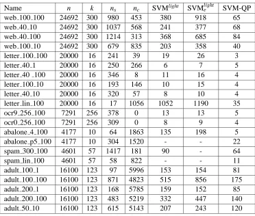
Name n k ns nc SVMlight SVMlighte SVM-QP web 100 100 24692 300 980 453 380 918 65 web 40 10 24692 300 1037 568 241 377 68 web 40 100 24692 300 1214 313 368 685 84 web 100 10 24692 300 679 835 203 358 40 letter 100 100 20000 16 241 39 19 26 3 letter 40 1 20000 16 250 266 6 7 5 letter 40 100 20000 16 346 8 11 16 4 letter 100 10 20000 16 193 146 10 15 4 letter 40 10 20000 16 320 57 8 10 4 letter lin 100 20000 16 17 1056 1052 1190 35 ocr9 256 100 7291 256 378 0 13 13 5
ocr0 256 100 7291 256 309 0 8 9 4
abalone 4 100 4177 10 64 1863 135 198 5 abalone p5 100 4177 10 304 1520 - - 22 spam 300 100 4601 57 1417 181 90 - 64 spam lin 100 4601 57 58 822 - - 11 adult 100 1 16100 123 97 5996 153 154 81 adult 100 100 16100 123 871 4823 515 856 175 adult 200 1 16100 123 168 5785 159 152 85 adult 200 100 16100 123 483 5219 332 447 140 adult 50 10 16100 123 615 5143 207 243 120
Table 1: Performance comparison of SVM-QP and SVMlight.
We chose CPU time (in seconds) as the most reasonable performance measure in our setting. The “-” in the table indicates the failure of SVMlighton that problem.
Table 1 contains the results for the test problems that we examine in this paper. As we can see, SVM-QP is faster than even the lower accuracy SVMlight, on all of the problems. It is faster by at least a factor of 2 on almost all of the problems and by a factor of 5 or more on a few problems.
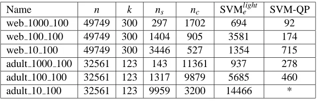
In Table 2 we present the comparison of SVM-QP and SVMlight on the full test sets for adult and web. These results were obtained by Hans Mittleman, at Arizona State University using a high-end Unix workstation. The “*” in the last column of the last row indicates that SVM-QP ran out of memory, since it was trying to store an ns×nsmatrix, with ns≈10000. The stopping tolerance was set to be 10−6for both codes, but it is interesting to note that the resulting support vector sets differed significantly. For example, the number of active support vectors for web 10 100 reported by SVM-QP was 3446, while the same number reported by SVMlight was 4025. This discrepancy is due to the fact that SVMlight converges to the optimal active set asymptotically, while SVM-QP steps from one feasible active set to another in an “exact” manner, until the optimal is found.
4. Implementation Issues
Name n k ns nc SVMlighte SVM-QP web 1000 100 49749 300 297 1702 694 92 web 100 100 49749 300 1404 905 3581 174 web 10 100 49749 300 3446 527 1354 715 adult 1000 100 32561 123 143 11361 937 278 adult 100 100 32561 123 1317 9879 5685 460 adult 10 100 32561 123 9959 3200 14466 *
Table 2: Performance comparison of SVM-QP and SVMlight on large data sets.
4.1 Selecting the Incoming Element of Is
In this subsection we discuss the implementation of Step 2(i). First of all we note that the compu-tational cost of Step 2(i) depends on whether the kernel values are available in the memory or have to be computed. We need O(|Is|(|I00|+|Ic0|))kernel values at each iteration when Step 2 is invoked. Specifically we need the elements of matrix Q whose column indices are in Isand whose row indices are in Ic0 and I00.
We note that we always store the ns×nsmatrix Qss. This can be a problems when nsis large. Our algorithm requires storage of the Cholesky factor of Qss, hence even if we do not store Qss itself, the storage requirement can be reduced at most by half. In our experiments the size of Qss and its Cholesky factor was reasonable. For extremely large problems a different implementation may be necessary which solves the linear system in Step 1 by an iterative solver.
To reduce the computational cost it is best to be able to store the entire Qs matrix (that is the submatrix of Q whose column indices are in Is). In some cases this might be prohibitively expensive in terms of memory. In our experiments we were able to store Qsin the space not exceeding 400MB. At the end of this subsection we will discuss the memory saving version of our code.
Let us assume for now that matrix Qs is available. We will consider various ways of reducing the number of elements in I00 and Ic0 at each repetition of Step 2(i). One simple way to achieve this is to compute the elements of s00 and ξ0c until a negative element is encountered, hence, not looking for the maximum violation, but for any violation. This may reduce the per-iteration time, but greatly increases the number of iterations, as has been shown by the extensive practice of the Simplex method in linear programming (Vanderbei, 2001). We will demonstrate this in the section on the incremental mode, since the incremental mode lacks the ability to “look ahead” and select the maximum violated constraint. We conclude that it is important to select the most negative or nearly the most negative element of s00andξ0cduring Step 2.
We use the following concepts, common in LP literature. The primal slack and surplus variables siandξiare the reduced costs of the associated dual variableαi, whose value is currently at a bound. Computing the values of the reduced costs (recall that for each i only one of the reduced costs is not equal to zero) is calledpricing of the appropriate dual variable. Hence it is important to price all variables with indices in I00 and Ic0 and maintain these sets in such a way that they contain indices of substantially negative reduced costs.
Ic0are large, while Isis not very small, then the complexity of this step, which is O(|Is|(|I00|+|Ic0|)), might become too high.
Let us assume for a moment that we know some of the indices that at optimality belong to Ic and I0. Then we can place these indices in I000 and Ic00 at the beginning of each Step 2. This can result in substantial savings in the run time, since Step 2(i) requires O(|Is|(|I00|+|Ic0|))operations and|I00|=|I0| − |I000|and|Ic0|=|Ic| − |Ic00|. When all the reduced costs of variables whose indices are in I00and Ic0are nonnegative, then so are the reduced costs of variables whose indices are in I000 and Ic00, due to our assumption about these two subsets.
Naturally, we usually do not know which indices will be in I0 and Ic at optimality, however, to reduce the workload at each iteration we try to guess which indices are the most likely ones to end up in I0 and Ic at optimality. We place such indices in I000 and Ic00 sets, respectively. If we guess well, then after all the reduced costs for I00and Ic0become nonnegative, hopefully, only a few reduced costs for I000and Ic00are negative. Here we see a trade-off: if we select I000and Ic00too small, then the computational saving is insignificant, and if we select I000and Ic00 too large, then some of large negative reduced costs might be missed and the overall number of iterations might increase. Moreover, once all the dual variables with indices in I00and Ic0are priced, then we have to price all variables with indices in I000and Ic00, which are large. So it is important to choose I000and Ic00in such a way that pricing the variables in I000and Ic00does not occur too many times.
We will describe two possible strategies for maintaining sets I00, Ic0, I000 and Ic00. One strategy is very simple and is called shrinking in SVM literature (Joachims, 1999). At each iteration an index is placed in I000or Ic00if its appropriate reduced cost remained nonnegative for a given number of consecutive iterations (say 100). According to this strategy the sets I00 and Ic0 are large during the earlier iterations and become gradually smaller during the course of the algorithm. This nicely correlates with the fact that the size of Isis very small in the earlier iterations Isgets gradually larger during the course of the algorithm. It is often the case that maximum of |Is|(|I00|+|Ic0|) over all iteration is 3 or 4 times smaller than max{|Is|} ×max{(|I00|+|Ic0|)}. At the end one still has to price all the dual variables for I000and Ic00, but only a few of such iterations are usually needed.
The second strategy is called sprint in Linear Programming literature and was introduced by Forrest (1989). Sprint (sometimes also called sifting) has been proven to be very effective in practice for problems that contain large number of inactive constraints (see Bixby et al., 1992). Following the sprint strategy we select a relatively small subset of dual variables with the smallest (including the most negative) reduced costs and we form I00 and Ic0 from the indices of those variables. Once the problems was solved for I00and Ic0the remaining constraints are priced again and the next relatively small sets of candidates are selected. Pricing all remaining variables and choosing the next small subset is called amajor iteration. According to this strategy I00 and Ic0 are always kept small, but the sets I000and Ic00have to be considered regularly throughout the algorithm. As long as the ratio of major iterations to the number of “cheap” iterations is small, the implementation will be efficient.
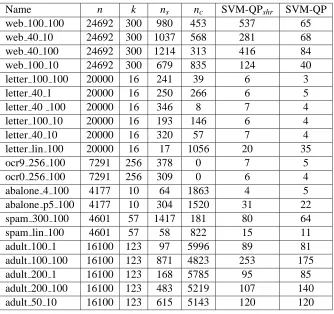
Table 3 below shows that sprint outperforms shrinking in most cases, especially on larger, more difficult problems.
4.2 Memory Saving Version
Name n k ns nc SVM-QPshr SVM-QP web 100 100 24692 300 980 453 537 65 web 40 10 24692 300 1037 568 281 68 web 40 100 24692 300 1214 313 416 84 web 100 10 24692 300 679 835 124 40 letter 100 100 20000 16 241 39 6 3 letter 40 1 20000 16 250 266 6 5 letter 40 100 20000 16 346 8 7 4 letter 100 10 20000 16 193 146 6 4 letter 40 10 20000 16 320 57 7 4 letter lin 100 20000 16 17 1056 20 35 ocr9 256 100 7291 256 378 0 7 5 ocr0 256 100 7291 256 309 0 6 4 abalone 4 100 4177 10 64 1863 4 5 abalone p5 100 4177 10 304 1520 31 22 spam 300 100 4601 57 1417 181 80 64 spam lin 100 4601 57 58 822 15 11 adult 100 1 16100 123 97 5996 89 81 adult 100 100 16100 123 871 4823 253 175 adult 200 1 16100 123 168 5785 95 85 adult 200 100 16100 123 483 5219 107 140 adult 50 10 16100 123 615 5143 120 120
Name n k ns nc SVM-QP SVM-QPmem SVMlightmem web 100 100 24692 300 980 453 65 428 1097 web 40 10 24692 300 1037 568 68 447 553 web 40 100 24692 300 1214 313 84 524 1201 web 100 10 24692 300 679 835 40 230 348 letter 100 100 20000 16 241 39 3 14 26
letter 40 1 20000 16 250 266 5 17 9
letter 40 100 20000 16 346 8 4 17 15 letter 100 10 20000 16 193 146 4 14 14 letter 40 10 20000 16 320 57 4 20 11 letter lin 100 20000 16 17 1056 35 72 1052
ocr9 256 100 7291 256 378 0 5 24 13
ocr0 256 100 7291 256 309 0 4 13 9
abalone 4 100 4177 10 64 1863 5 13 78 abalone p5 100 4177 10 304 1520 22 44 -adult 100 1 16100 123 97 5996 81 171 228 adult 100 100 16100 123 871 4823 175 624 1541 adult 200 1 16100 123 168 5785 85 174 253 adult 200 100 16100 123 483 5219 140 173 1360 adult 50 10 16100 123 615 5143 120 355 593
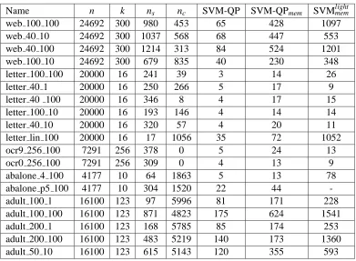
Table 4: Comparison for memory saving mode.
the user. In the experiments discussed above we allowed the size of the cache to be 500MB, which is at least as much memory as was used by SVM-QP.
We did not implement such sophisticated memory handling mechanism in our code. Luckily sprint provides a natural setting for a memory saving mode. Instead of storing the whole Qs we only store the elements of Q whose columns are in Isand whose rows are in Is∪I00∪Ic0. The size of I00∪Ic0 can be regulated according to the available storage space. At each major iteration all the elements of Qswhose row indices are in I000∪Ic00have to be recomputed. This can be a costly step. To further try to reduce the computational cost of that step, we applyshrinking to I000∪Ic00. That is, if during a few consecutive major iterations a certain reduced cost remained nonnegative then the appropriate variable is removed from I000∪Ic00and is ignored until the later stage of the algorithm. In Table 4 below we present our results. We chose the size of I00 and Ic0to be 50 each, this way the total storage for the elements of Qs(including Qss) did not exceed 20MB. We compare our CPU time to that of SVMlight with 20MB of cache limit. We also list the CPU times for the version of SVM-QP that stores the full Qs, to demonstrate the trade-off between the CPU time and memory requirement.
4.3 Warm Start
and the new optimal solution is typically obtained within a few iterations. This will be explored in more detail in the subsection on the incremental mode of our algorithm.
Another situation where warm start arises, is when one wants to explore the path of optimal solutions for various values of penalty parameter C. In Hastie et al. (2004) the whole solution path is generated using an active set method similar to ours. There some differences between the two methods, however. The method in Hastie et al. (2004) is a parametric active set method, which in practice is usually slower than a purely primal or dual active set method, such as ours. Also their method requires that at each iteration an optimal solution of a parametric problem is available, hence there does not seem to be any possibility to use sprint or shrinking. It remains to be seen whether a good implementation of the algorithm in Hastie et al. (2004) can match the performance of our algorithm.
Our algorithm is not suitable directly for generating the entire parametric path, but using the warm starts one can easily use it to generate solutions for a selection of the values of parameter C.
The warm starts can also be used when one wants to explore different values of kernel parame-ters, but the efficiency of such application needs a separate computational study.
Here we investigate the use of warm start to increase the efficiency of the algorithm itself. It has been noticed (see, for example, Fine and Scheinberg, 2001) that for many SVM problems the matrix Q has eigenvalues decaying to zero. It was suggested in Fine and Scheinberg (2001) to use a low rank approximation of Q and solve the approximate problem with an interior point method using product form Cholesky factorizations, which benefit from the low rank of Q. Such approximations, however, are not always very accurate. The idea we explore here is to use the solution of the approximate problem to warm start the active set method.
If k is the rank of the approximation of Q, then per iteration complexity of the IPM is O(nk2). There is a trade-off in choosing the right value for k: if k is chosen to be too large, then the IPM will not be efficient and if k is too small then the solution produced by the IPM is too far from the optimal solution of the true problem. We chose k=50, which is reasonably small to make the IPM part fast and sufficiently large to hope for a good warm start. The results in Table 5 are not as dramatic as one might hope. Often the active set method itself is so fast that it outperforms the IPM even for k=50, for instance on letter x x problems. In other cases the approximation does not produce a good enough warm start. There also cases where Q itself has very low rank and, hence, the problem can be solved to optimality just by the IPM; see letter lin 100, for instance. There are examples however, where the combined method achieves better timing results than either method, when used separately. This seem to happen for the problems with relatively large Icsets, such as the adult x x problems. We have to note that we are using a rather crude implementation of the IPM for SVM. One might achieve better results with a more efficient implementation of an IPM.
4.4 Incremental Mode
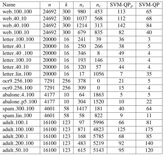
Name n k ns nc SVM-QPp SVM-QP web 100 100 24692 300 980 453 113 65 web 40 10 24692 300 1037 568 112 68 web 40 100 24692 300 1214 313 142 84 web 100 10 24692 300 679 835 82 40 letter 100 100 20000 16 241 39 36 3 letter 40 1 20000 16 250 266 38 5 letter 40 100 20000 16 346 8 49 4 letter 100 10 20000 16 193 146 33 4 letter 40 10 20000 16 320 57 44 4 letter lin 100 20000 16 17 1056 7 35 ocr9 256 100 7291 256 378 0 21 5 ocr0 256 100 7291 256 309 0 15 4 abalone 4 100 4177 10 64 1863 5 5 abalone p5 100 4177 10 304 1520 10 22 spam 300 100 4601 58 1417 181 40 64 spam lin 100 4601 58 58 822 9 11 adult 100 1 16100 123 97 5996 66 81 adult 100 100 16100 123 871 4823 125 175 adult 200 1 16100 123 168 5785 68 85 adult 200 100 16100 123 483 5219 92 140 adult 50 10 16100 123 615 5143 95 120
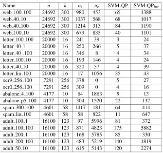
Name n k ns nc SVM-QP SVM-QPinc web 100 100 24692 300 980 453 65 1388 web 40 10 24692 300 1037 568 68 1017 web 40 100 24692 300 1214 313 84 1190 web 100 10 24692 300 679 835 40 1101 letter 100 100 20000 16 241 39 3 24 letter 40 1 20000 16 250 266 5 37 letter 40 100 20000 16 346 8 4 34 letter 100 10 20000 16 193 146 4 24 letter 40 10 20000 16 320 57 4 39 letter lin 100 20000 16 17 1056 35 43 ocr9 256 100 7291 256 378 0 5 27 ocr0 256 100 7291 256 309 0 4 16 abalone 4 100 4177 10 64 1863 5 13 abalone p5 100 4177 10 304 1520 22 137 spam 300 100 4601 58 1417 181 64 414 spam lin 100 4601 58 58 822 11 647 adult 100 1 16100 123 97 5996 81 372 adult 100 100 16100 123 871 4823 175 5882 adult 200 1 16100 123 168 5785 85 330 adult 200 100 16100 123 483 5219 140 1819 adult 50 10 16100 123 615 5143 120 2274
Table 6: Incremental mode.
with sufficiently negative reduced costs are not included, until their data points are added to the problem. As we show in Table 6, this results in a dramatic increase of CPU time.
Notice, that the sifting does not make sense in the incremental mode, since it selects the sets I00 and Ic0based on the entire data set. However, shrinking can be easily applied, since its selection of I00and Ic0is only based on the past behavior of each individual constraint.
5. Concluding Remarks
Traditional active set methods for convex QPs were considered impractical for large-scale SVM problems. However, they have theoretical appeal for many reasons. In this paper we studied in details an active set method SVM and show that an efficient implementation can outperform other state-of-the-art SVM software.
Acknowledgments
The author is grateful to Alexandre Belloni for pointing out the paper (Frangioni, 1996) for handling the singular reduced QP system as well as for many fruitful discussions. The author is also grateful to John Forrest for suggesting the sprint technique.
References
J. Balcazar, Y. Dai, and O Watanabe. Provably fast trainning algorithms for support vector machines. In Proc. 1st IEEE International Conference on Data Mining, pages 43–50. IEEE, 2001.
R. E. Bixby, J. W. Gregory, I. J. Lustig, R. E. Marsten, and D. F. Shanno. Very large-scale lin-ear programming: A case study in combining interior point and simplex methods. Operations Research, 40(5):885–897, 1992.
C. L. Blake and C. J Merz. UCI repository of machine learning databases, 1998. URL
http://www.ics.uci.edu/∼mlearn/MLRepository.html.
B. Boser, I. Guyon, and V. N. Vapnik. A training algorithm for optimal margin classifiers. In D. Haussler, editor, Proceedings of the 5th Annual ACM Workshop on Computational Learning Theory, pages 144–152. ACM Press, 1992.
G. Cauwenberghs and T. Poggio. Incremental and decremental support vector machine learning. In Todd K. Leen, Thomas G. Dietterich, and Volker Tresp, editors, Advances in Neural Information Processing Systems 13, pages 409–415. MIT Press, 2001.
N. Cristianini and J. Shawe-Taylor. An Introductin to Support Vector Macines and Other Kernel-Based Learning Methods. Cambridge University Press, 2000.
M. C. Ferris and T. S. Munson. Interior point methods for massive support vector machines. Techni-cal Report 00-05, Computer Sciences Department, University of Wisconsin, Madison, WI, 2000.
S. Fine and K. Scheinberg. Efficient svm training using low-rank kernel representations. Journal of Machine Learning Research, 2:243–264, 2001.
R. Fletcher. A general quadratic programming algorithm. Journal of the Institute of Mathematics and Its Applications, pages 76–91, 1971.
J. J. Forrest. Mathematical programming with a library of optimization subroutines. Presented at the ORSA/TIMS Joint National Meeting, 1989.
A. Frangioni. Solving semidefinite quadratic problems within nonsmooth optimization algorithms. Computers in Operations Research, 23(11):1099–1118, 1996.
D. Goldfarb. Extension of newton’s method and simplex method for solving quadratic problems. In F. A. Lootsma, editor, Numerical Methods for Nonlinear Optimization, pages 239–254. Academic Press, London, 1972.
G. H. Golub and Ch. F. Van Loan. Matrix Computations. The Johns Hopkins University Press, Baltimore and London, 3rd edition, 1996.
T. Hastie, S. Rosset, R. Tibshirani, and J. Zhu. The entire regularization path. Journal of Machine Learning Research, 5:1391–1415, 2004.
T. Joachims. Making large-scale support vector machine nlearning practicle. In B. Sch ¨olkopf, C. C. Burges, and A. J. Smola, editors, Advances in Kernel Methods, chapter 12, pages 169–184. MIT Press, 1999.
L. Kaufman. Solving the quadratic programming problem arising in support vector classification. In B. Sch¨olkopf, C. C. Burges, and A. J. Smola, editors, Advances in Kernel Methods Support Vector Learning, pages 147–168. MIT Press, 1998.
K. C. Kiwiel. A dual method for certain positive semidefinite quadratic programming problems. SIAM Journal on Scientific and Statistical Computing, 10:175–186, 1989.
J Nocedal and S. Wright. Numerical Optimization. Springer-Verlag, 1999.
E. Osuna, R. Freund, and F. Girosi. An improved training algorithm for support vector machines. In Proceedings of the IEEE Neural Networks for Signal Processing VII Workshop, pages 276–285. IEEE, 1997.
J. C. Platt. Fast trining support vector machines using sequential mininal optimization. In B. Sch¨olkopf, C. C. Burges, and A. J. Smola, editors, Advances in Kernel Methods, chapter 12, pages 185–208. MIT Press, 1999.