1 Jed Long
1
University of St Andrews 2
St. Andrews, Fife 3
Long and Nelson · Home Range and Dynamic Time Geography 5
Home Range and Habitat Analysis using Dynamic Time Geography 6
JED LONG,1Department of Geography and Sustainable Development, University of St Andrews, St
7
Andrews, Fife, United Kingdom
8
TRISALYN NELSON, Department of Geography, University of Victoria, Victoria, British Columbia,
9
Canada
10
11
1
Email: [email protected] Pre-print of published version.
Reference:
Long, JA, TA Nelson. 2015. Home range and habitat analysis using dynamic time geography. Journal of Wildlife Management.
DOI:
http://dx.doi.org/10.1002/jwmg.845
Disclaimer:
2 ABSTRACT Wildlife home ranges continue to be a common spatial unit for modeling animal habitat 12
selection. Telemetry data are increasing in spatial and temporal detail and new methods are being 13
developed to incorporate fine resolution data into home range delineation. We extended a previously 14
developed home range estimation technique that incorporates theory from time geography, the potential 15
path area (PPA) home range, to allow the home range to be defined at multiple spatial scales depending 16
on the observed rate of movement within the data. The benefits of this approach are demonstrated with 17
a simulation study, which uses multi-state correlated random walks to represent dynamic movement 18
phases to compare the modified PPA home range technique with a suite of other home range estimation 19
methods (PPA home range, kernel density estimation, Brownian bridges, and dynamic Brownian 20
bridges). We used a case study on caribou (Rangifer tarandus) movement from northern Canada to 21
highlight the value of this approach for characterizing habitat conditions associated with wildlife 22
habitat analysis. We used a simple habitat covariate, percent forest cover, to explore the potential for 23
misleading habitat estimates when home ranges do not include potentially visited locations (omission 24
area) or include areas not possibly visited (commission area). We highlight the advantages of the 25
dynamic PPA home range in the context of quantifying omission and commission areas in other home 26
range techniques. Finally, we provide our R code for calculating dynamic PPA home range estimates. 27
KEY WORDS caribou (Rangifer tarandus), commission area, correlated random walk, omission area, 28
telemetry. 29
3 With continued development of spatial tracking technologies (e.g., global positioning system [GPS], 32
Argos), unprecedented datasets are facilitating novel research on wildlife movement and behavior. 33
These improvements have resulted in wildlife telemetry data with finer sampling intervals, over longer 34
temporal extents, and with better spatial accuracy (Cagnacci et al. 2010). Improved spatial and 35
temporal resolution of telemetry data have provided scientists the opportunity to conduct increasingly 36
detailed analysis of animal movement and the potential to answer increasingly sophisticated questions 37
regarding wildlife biology, behavior, and response to change (Patterson et al. 2008). 38
The home range continues to be a primary spatial unit for wildlife analysis and modeling (Beyer 39
et al. 2010). The most oft-cited definition of a home range is the area to which an animal confines its 40
normal movements (Burt 1943). However, a robust mathematical formulation of this definition is still 41
absent, and the practical definition of a home range is dependent on the chosen method for estimating it 42
(Fieberg and Börger 2012). Thus, there are many approaches for estimating wildlife home ranges, for 43
example minimum convex polygons, kernel density estimation (Worton 1989), local convex hulls (Getz 44
and Wilmers 2004), and Brownian bridges (Horne et al. 2007). 45
Home ranges are a useful summary unit for spatial analysis of wildlife movement because they 46
explicitly relate to processes (such as territoriality, spatial memory, and habitat preference) associated 47
with space-selection patterns in many wildlife species (Börger et al. 2008, Van Moorter et al. 2009). As 48
a conservation tool, home ranges represent a useful spatial unit for management decision-making and 49
analysis (Reynolds et al. 1992, Bull and Holthausen 1993, Linnell et al. 2001). Home ranges are 50
commonly used in 2 areas of spatial analysis: to quantify differences in home range areas and to study 51
habitat selection. Quantifying differences in home range areas, for example between sexes (Swihart and 52
Slade 1989), or over time (Smulders et al. 2012) provides insight into wildlife movement processes 53
associated with spatial selection and mobility. Habitat analysis using home ranges links spatial 54
4 Analyzing changes in home range estimates, or the habitat variables associated with them, is 56
complicated by the presence of areas of omission and commission error. Omission and commission 57
areas are defined, respectively, as habitat used by the animal that is excluded from the home range and 58
habitat that is unused but included in the home range (Sanderson 1966). Similarly, Getz and Wilmers 59
(2004) refer to Type I error as including invalid areas and Type II error as excluding valid areas in 60
home range estimates. Home range estimation methods that reduce omission and commission areas, or 61
methods that can be used to quantify these areas in existing methods, are necessary to improve wildlife 62
home range studies. However making comparisons across home ranges is difficult with empirical data 63
because there is no truth for comparison and each method places different assumptions on the data. 64
The potential path area (PPA; Long and Nelson 2012) approach takes an alternative view on 65
home range estimation, one based on a time geographic view of individual movement (Hägerstrand 66
1970). Within the time geographic framework, movement opportunities are represented using a space-67
time prism, which is a 3-dimensional (space and time) volume that contains all potential movement 68
paths between 2 known telemetry fix locations (Fig. 1). The space-time prism represents a useful 69
measure for understanding the spatial-temporal constraints on individual movement opportunity (Kwan 70
1999) and for this reason is commonly referred to as the accessibility space (Kwan 1998). The PPA is 71
the projection of the space-time prism onto the spatial plane, and represents a purely spatial measure of 72
accessibility (Fig. 1). The PPA home range is calculated by recursively computing PPA ellipses for 73
consecutive pairs of telemetry locations, which are then combined (using a spatial union) to estimate 74
the home range (see Long and Nelson 2012). The PPA home range estimate focuses explicitly on the 75
delineation of the accessibility space of the individual, which makes it a useful spatial unit for 76
comparing across methods in the context of omission and commission areas. 77
The size and shape of the space-time prism, and thus the PPA home range estimate, depends on 78
the time between locations and a mobility parameter vmax, which can be interpreted as a maximum
5 travel velocity. In some cases, vmax may be known based on a fine understanding of organism biology.
80
In most cases, vmax must be estimated from the telemetry data; for example Long and Nelson (2012)
81
outline several statistical procedures that can be used to estimate vmax, which are derived from methods
82
for estimating the upper bound of a distribution given a set of values. With the PPA approach, vmax is a
83
global parameter applied to the entire telemetry dataset (i.e., all pairs of points). With organisms that 84
exhibit highly variable mobility levels, PPA home range estimates will overestimate home range area 85
for periods of lower mobility, leading to increased commission areas, a problem also encountered with 86
other methods (e.g., from over-smoothing; Gitzen et al. 2006, Downs and Horner 2008). A dynamic 87
vmax parameterization incorporating higher and lower mobility levels will reduce over-estimation of
88
home range areas associated with low mobility phases, and reduce commission area. 89
Explicitly considering wildlife movement phases is one approach to reducing omission and 90
commission areas (Kranstauber et al. 2012). Kernel and minimum convex polygon approaches, for 91
instance, cannot include movement phases because they ignore the temporal component of telemetry 92
data. Most wildlife species exhibit multiple movement phases, often linked to different behaviors, 93
resulting in variation in patterns and scales of movement, as well as habitat selection. A number of 94
robust statistical techniques currently exist that can be used to identify different movement phases 95
within a telemetry dataset (e.g., latent models: Morales et al. 2004, Jonsen, Flemming and Myers 2005; 96
change-point analysis: Gurarie et al. 2009). Within each phase, movement parameters should follow a 97
similar pattern, whereas between phases movement parameters shift dramatically from, for example, 98
low motion (resting) to high motion (migration) states. To reduce omission and commission areas, 99
space-time variation associated with different movement phases may be useful for refining home range 100
estimates, and subsequently, habitat selection studies. 101
We extended the PPA approach by dynamically modeling the mobility parameter (vmax) so that
102
6 We call the extension the dynamic potential path area home range (dynPPA). Using simulated data and 104
empirical caribou (Rangifer tarandus) telemetry data, we demonstrate how the dynPPA approach 105
provides an alternative measure of animal space use and a useful comparison metric among existing 106
home range techniques for quantifying omission and commission areas. Finally, we provide an R-based 107
toolset for performing dynPPA analysis. 108
METHODS 109
Dynamic PPA Home Range (dynPPA) 110
We follow Long and Nelson's (2012) method of estimating vmax from a telemetry dataset of n fix
111
locations for a single individual. Estimates of vmax are a function of the distribution of individual
112
segment velocities (vi) given by:
113 i i i t d
v [1]
114
where di is the distance and ti the time between consecutive fixes. Based on the distribution of the vi for
115
the entire trajectory, vmax is an upper bound on the vi, which can be estimated by several statistical
116
estimation techniques (e.g., Robson and Whitlock 1964, van der Watt 1980). For example Long and 117
Nelson (2012) suggest the method described by van der Watt (1980) which considers the ordered set of 118
the visuch that v1 < v2 < …< vm-1< vm and m = n − 1.
119 k m m v k v k k
v
1 1 1 2
m ax [2]
120
where 1 < k < m represents the kth ordered value of vi. We extend the vmax estimation procedure from
121
Long and Nelson (2012) to account for behavioral shifts throughout the tracking period. Thus, dynamic 122
vmax is defined by a similar function:
123
i pp F v
vm ax, , [3]
124
Where vmax,p is the vmax estimate for the pth dynamic phase comprising of a subset of the n telemetry
125
fixes and F(vi, p) is a statistical technique (e.g., [2]) for estimating the upper-bound of a distribution
7 applied to the vi in phase p. The phases (p) may be from a temporally dynamic moving window, or
127
associated with discrete behavioral phases. Although we used the technique described in van der Watt 128
(1980), this approach can be used with other functions for estimating the upper-bound of a distribution. 129
Importantly, such a dynamic calculation of the PPA (dynPPA) home range estimate allows for 130
variations in the vmax parameter through time resulting from changes in movement behavior.
131
The construction of the dynPPA home range explicitly considers the movement ability of the 132
individual animal to delineate their accessibility space throughout the movement trajectory. Thus, by 133
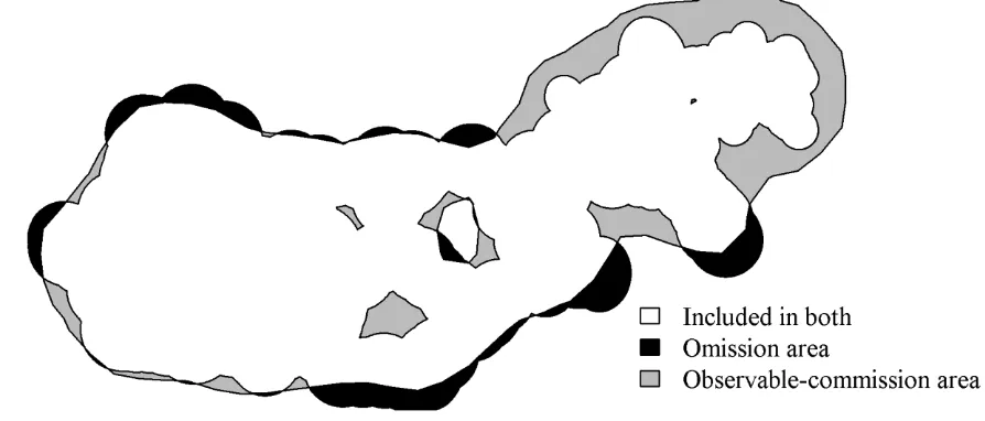
taking a spatial overlay of the dynPPA and other home range estimators, we define areas included in the 134
dynPPA home range but not included in home range estimates from other methods as omission area 135
(Fig. 2); these are areas that were accessible to the animal but not included in the home range estimates 136
from the other methods. Omission area is prevalent in most methods, and is included in the commonly 137
accepted definition of a home range (i.e., the occasional sallies described by Burt 1943). Quantifying 138
commission area is not as straightforward, because all home range estimates are likely to include 139
locations not actually visited by the animal because of the incomplete nature of telemetry data. We 140
define areas included in the home range estimates from other methods but not included in the dynPPA 141
home range as observable-commission areas, which represent areas included in the home range but 142
outside of the accessibility space of the animal (Fig. 2). Observable-commission areas represent 143
locations the animal could not possibly have visited given the known fix locations and an upper-bound 144
on mobility (vmax). For example, the presence of high-levels of observable-commission area is one of
145
the main reasons why minimum convex polygons are problematic with irregularly shaped patterns of 146
animal telemetry data (Harris et al. 1990, Barg et al. 2004). Through the analysis of these spatial 147
differences, we show how the dynPPA home range method improves upon the original PPA model and 148
provides a unique and complementary view to home range estimation by explicitly delineating the 149
8 accounting for changes in mobility relating to dynamic movement behavior. Further, dynPPA home 151
range can be used to evaluate and refine home range estimates from other methods through the 152
quantification of spatial differences, which we define as omission and observable-commission areas. 153
Other Home Range Methods 154
Many methods exist for computing wildlife home ranges; we focus on comparing the original PPA 155
method, 3 more popular current approaches – kernel density estimation (KDE; Worton 1989), 156
Brownian bridges (BB; Horne et al. 2007), and dynamic Brownian bridges (dynBB; Kranstauber et al. 157
2012) – and the new dynPPA approach. With KDE, BB, and dynBB, the home range is a 2-dimensional 158
projection of the utilization distribution of the animal from which a percent volume contour is extracted 159
to delineate home range as a polygon. Kernel density estimation relies on the selection of a suitable 160
kernel bandwidth, which remains a highly contentious issue in home range analysis (Hemson et al. 161
2005, Fieberg 2007). The Brownian bridge approach models movement as a Brownian diffusion 162
process anchored on 2 consecutive fixes. The n-1 Brownian bridges are combined to produce the BB 163
home range, and in this sense it is comparable to the PPA approach. The BB home range requires the 164
selection of 2 variance parameters, one related to uncertainty in fix locations, and the other termed the 165
Brownian motion variance, which is related to the mobility of the animal. The Brownian motion 166
variance parameter is estimated globally from the entire telemetry dataset (of an individual) using a 167
leave-one-out estimation process (Horne et al. 2007). To generalize the BB approach, Kranstauber et al. 168
(2012) developed the dynBB, which uses a temporally varying estimate of the Brownian motion 169
parameter to account for dynamic movement phases. 170
Simulation Study 171
We simulated 1,000 correlated random walks (CRW) to compare home range estimation techniques. 172
Correlated random walks rely on 2 parameters. The first (r) governs the level of serial correlation in 173
9 dynamic movement behavior, we varied the number of distinct movement phases (p) within each
175
simulated CRW between 5 and 10. For each movement phase, CRW parameters were chosen randomly 176
but restricted in such a way that higher mobility phases (h = 3 to 5) were associated with more directed 177
(i.e., correlated) movements (r = 0.3 to 0.7), and lower mobility phases (h = 1 to 3) were associated 178
with more random movements (r = 0 to 0.4). 179
For each simulated CRW, we computed the potential path area home range (PPA), the 95% 180
volume contour kernel density home range estimate, the 99% volume contour Brownian bridge home 181
range, the 99% volume contour dynamic Brownian bridge home range, and the dynamic PPA home 182
range. We computed kernel bandwidth for KDE using the half the reference bandwidth, a modification 183
that can reduce the effect of over-smoothing in KDE when data exhibits clumpy patterns (Worton 184
1995). We selected the 95% volume contour because it is the most commonly chosen level in past 185
home range studies (Laver and Kelly 2008) and is typically used to estimate the home range, whereas 186
lower values (e.g., 50%) are used to delineate core area. We computed the variance parameter for the 187
BB and dynBB models using the maximum likelihood method outlined by Horne et al. (2007) and 188
assumed the error parameter to be appropriately small. We chose a 99% volume contour level for the 189
BB and dynBB methods following Horne et al. (2007). 190
For each technique, we computed the home range area, plus the intersection area with the 191
dynPPA to examine spatial differences among methods. Results from the simulated study are presented 192
as percentages of the dynPPA for comparison purposes, thus making the area of the dynPPA home 193
range estimate the baseline areal measurement. 194
Case Study – Caribou in Northern British Columbia, Canada 195
To further demonstrate the dynPPA approach, we used a dataset of the movements of 4 caribou over the 196
course of a year (2001). The telemetry data were collected with a regular, 4-hour sampling interval, 197
10 of movement phases are generally unknown. We use the behavioral change point algorithm (BCPA: 199
Gurarie et al. 2009) to identify different movement phases for each individual caribou. The BCPA 200
requires 2 parameters. The first is the BCPA search window (w; Gurarie et al. [2009] suggest w > 30); 201
we used w = 43, approximately a 1-week interval in this example. The second parameter is a threshold 202
that identifies significant change points; we used 21, which is half of w, similar to that used by Gurarie 203
et al. (2009). We then computed the PPA, KDE, BB, dynBB, and dynPPA home ranges following the 204
methods for parameter estimation outlined in the simulation study. We again explore the presence of 205
omission and observable-commission area in various home range techniques in the caribou example 206
through area overlap comparisons with dynPPA. 207
We estimated the habitat composition (i.e., land cover) for each home range based on each 208
home range estimation method to examine the effect of method on the composition estimates. To 209
represent land cover, we used the Canada’s Earth Observation for Sustainable Development (EOSD) 210
dataset (Wulder et al. 2008), which was derived from Landsat satellite imagery. We selected percent 211
forest cover as an indicator of habitat because wooded areas are a primary habitat type for caribou, 212
especially outside of summer months (Wood 1994, Seip 1998). We focus on the percent forest cover 213
within each home range along with the sub-areas of the home range delineated as omission area and 214
observable-commission area to examine whether the composition of these sub-areas differed from the 215
overall home range, resulting in misleading composition estimates from home range methods. 216
RESULTS 217
Simulation Study 218
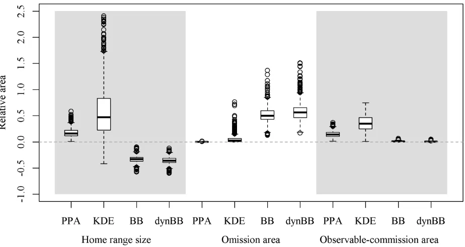
Our simulations revealed differences between estimated home range areas and the presence of omission 219
and observable-commission area across different home range methods (Fig. 3). The PPA approach 220
produced larger estimated home range sizes, as expected, whereas the BB and dynBB methods 221
11 estimates that could be either larger or smaller than dynPPA (Fig. 3). Omission area was greatest in the 223
BB and dynBB methods, but this is expected because these methods produced the smallest home range 224
estimates. In many situations, KDE also produced a substantial level of omission area, which is 225
surprising given that in general KDE produced the largest home range size estimates. As expected 226
based on definitions, omission area in the PPA was 0 because the PPA home range contains the dynPPA 227
home range. 228
In all simulations, PPA and KDE produced an observable-commission area (Fig. 3). Of these, 229
790/1,000 of the simulation PPA home ranges and 975/1,000 of the simulation KDE home ranges 230
contained observable-commission area comprising greater than 10.0% of the estimated home range. 231
The average percentage of observable-commission area was highest in KDE at 36.2%, with an average 232
of 14.6% for PPA. The BB and dynBB methods also produced some level of observable-commission 233
area in nearly all simulations (998/1,000 and 997/1,000 simulations, respectively). However, neither 234
method produced a simulation where the amount of observable-commission area was greater than 10% 235
proportionally of the home range area. The average observable-commission area was small in BB and 236
dynBB (1.2% and 0.7%, respectively). Overall, BB and dynBB compare best with dynPPA, likely 237
owing to similar derivations based on the sequence of telemetry fixes (path-based), producing similar 238
sizes and minimizing observable-commission area. 239
Case Study – Caribou in Northern British Columbia, Canada 240
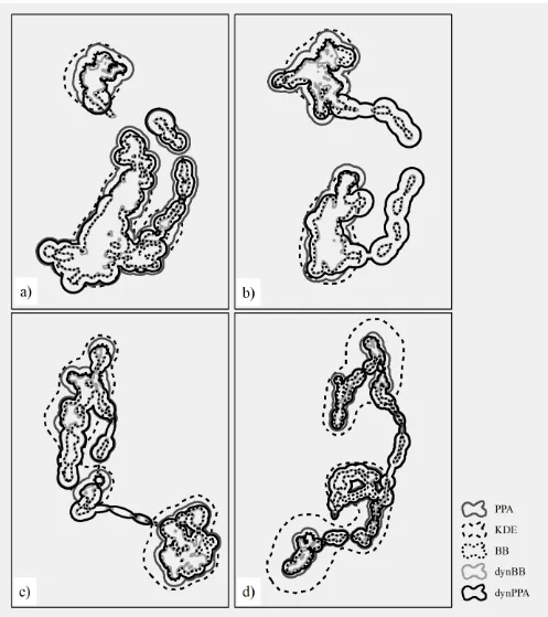
The 4 caribou in northern British Columbia, whose data we analyzed, exhibited similar movement 241
patterns consisting of 2 spatially disjoint seasonal ranges connected via movement corridors (Fig. 4). 242
Estimated home range areas had similar patterns as seen in the simulation study, with larger estimated 243
home ranges from the PPA and KDE methods, and smaller estimated home ranges from the BB and 244
dynBB methods (Fig. 4). Kernel density estimation produced the largest estimated home ranges but 245
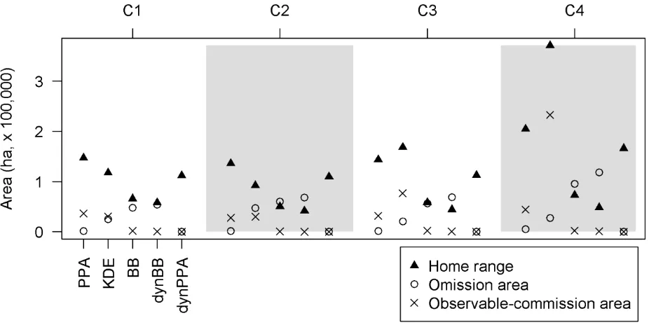
12 With the caribou dataset, the trend in estimated home range areas showed PPA or KDE being 247
largest, followed by dynPPA, BB, and dynBB (Fig. 5). In the case of caribou C4, the KDE home range 248
estimate was much larger owing to difficulty in specifying a suitable bandwidth using the objective 249
method chosen. The dynBB and BB methods are excellent at minimizing observable-commission areas, 250
and produce estimated home range sizes similar to each other. The KDE and PPA approaches both 251
produced substantial areas of observable-commission area, which is problematic in home range studies 252
because these areas are outside of the defined accessibility space of the animal. 253
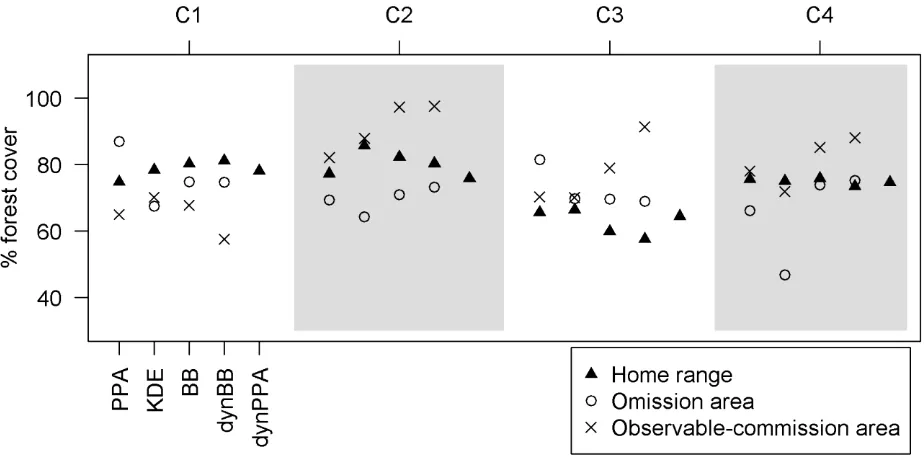
Estimated habitat composition revealed the potentially misleading effect of observable-254
commission areas (Fig. 6). For example, with the KDE method with data from caribou C2, the 255
observable-commission area was a substantial portion of the estimated home range, and the percent 256
forest cover was relatively high for this area. The high percent forest cover in the observable 257
commission area portion of the home range in C2 resulted in the highest observed percent forest cover 258
of all the home range methods, noticeably higher than any other estimates (Fig. 6). Conversely, in 259
caribou C4, the percent forest cover was similar in the observable-commission area to that of the 260
dynPPA home range, in this case leading to equivalent measures of percent forest cover, despite the 261
substantial overlap of home range size by the KDE method. The BB and dynBB methods produced 262
relatively small areas of observable-commission area, despite having substantial differences in percent 263
forest cover between the home range and observable-commission areas. However, in caribou C3, 264
estimates for percent forest cover were lower for the BB and dynBB methods because the omission 265
area had a higher percent forest cover, which shows the potentially misleading effect of omission area. 266
DISCUSSION 267
Concepts from time geography can be used to explicitly consider the elapsed time between telemetry 268
fixes, allowing home range estimation to use a path-based data representation (Long and Nelson 2012). 269
13 are point-based approaches, and define an enclosure or smooth a set of telemetry fixes. Point-based 271
methods use only the spatial geometry of telemetry fixes and thus may be hindered by the serially 272
correlated structure of modern telemetry datasets (Dray et al. 2010). Path-based methods for estimating 273
the home range leverage the temporal structure inherent in telemetry datasets. For example, methods 274
may consider consecutive telemetry fixes as anchor points in a diffusion (Brownian bridge) or 275
diffusion-drift process (biased random bridge; Benhamou 2011). The Brownian bridge and biased 276
random bridge methods delineate the utilization distribution of an individual based on random walk 277
theory, whereas the dynPPA home range method focuses on quantifying the polygon area accessible to 278
an individual given n telemetry fixes and a time-varying mobility parameter. 279
The dynPPA method takes an alternative view on estimating the home range, one that explicitly 280
considers that accessibility can be used to directly estimate the home range. That is, the dynPPA 281
delineates the area an animal could have visited based on a set of telemetry fixes and a time varying 282
mobility parameter vmax. We have demonstrated that dynPPA home range estimates can provide useful
283
stand-alone measures for estimating home range areas, comparable with popular existing methods. We 284
highlight the dynPPA approach as being simple and intuitive, but also stress how it can be used to 285
identify omission and observable-commission areas when comparing across multiple methods, a 286
practice increasingly common given the ease at which multiple methods can be implemented within a 287
single software (e.g., Calenge 2006). Specifically, because the dynPPA home range estimate focuses on 288
accessibility in its definition, we demonstrate how dynPPA can be used to quantify omission and 289
observable-commission area in other estimation techniques. Such comparisons are conditional on the 290
predication that the dynPPA estimate, which defines the individual accessibility space, represents a 291
suitable baseline for identifying omission and observable-commission area. 292
Wildlife researchers now have an array of computational tools from which to choose for 293
14 remains a need to define relatively straightforward spatial analysis units, drawing on the foundational 295
concept of the home range. The dynPPA home range method is based on different assumptions from 296
other home range approaches. We propose that because dynPPA explicitly considers accessibility in its 297
definition, it can be used for quantifying omission and observable-commission areas through direct 298
spatial comparisons of home range polygons. Further, many studies are interested in studying habitat 299
use versus habitat availability from telemetry data (Beyer et al. 2010). In use versus availability study 300
designs, the researcher must carefully consider how they define available habitat. At some scales, a 301
home range estimate (or a spatial extension of the home range such as a buffer around the home range) 302
is used to define potentially available habitat (Long et al. 2010). A time geographic approach (i.e., 303
dynPPA) is a logical method for identifying what constitutes available habitat in use versus availability 304
studies because dynPPA explicitly delineates accessible areas. 305
Our simulation study highlights the challenges with home range analyses that researchers have 306
been grappling with for decades: that different home range methods can lead to highly variable 307
estimates of home range size and configuration. When compared to other home range estimation 308
methods, dynPPA is generally larger than produced by BB or dynBB methods but smaller than for KDE 309
and the original PPA approach. From comparisons between home range estimates from other methods 310
with dynPPA, a researcher can decide whether a home range method is appropriate with a given 311
dataset, or re-evaluate the chosen parameter combinations. Our simulations can also be seen as further 312
evidence of the difficulty with KDE home range methods or more specifically the problem of 313
automated selection of the bandwidth (Hemson et al. 2005). In the simulation study, we use a popular 314
ad hoc method for identifying the kernel bandwidth (i.e., half the reference bandwidth), but the 315
resulting home range estimates were highly variable in size. When the home range is overestimated, the 316
result is substantial observable-commission area, which can be problematic when using home ranges 317
15 The results (both from the simulations and caribou study) confirmed that, like many home range 319
estimation methods, the original PPA approach (Long and Nelson 2012) may be overestimating home 320
range areas. We built on the ideas proposed by Kranstauber et al. (2012), that home range estimation 321
methods should consider different movement phases associated with variable movement parameters. 322
Thus, dynPPA is a generalization of the original PPA approach, where vmax is estimated independently
323
for each movement phase. This approach considers movement phases as discrete segments along the 324
trajectory, such that changes in movement parameters occur abruptly between phases (Kranstauber et 325
al. 2012) and typically represent a change in movement behavior (e.g., migrating vs. foraging). 326
Alternatively, movement parameters may vary continuously over time, and we have also implemented 327
a temporal moving-window approach for estimating vmax dynamically over time. We did not evaluate
328
the temporal moving-window method here but make it available with the R code provided to allow 329
researchers to use a moving-window approach should it be appropriate with their research (see 330
Supporting Information). 331
Methods for estimating movement parameters are complicated by missing fixes and irregular 332
fix intervals (see Laube and Purves 2011), issues commonly encountered in empirical wildlife 333
telemetry studies. Shorter than average fix intervals may be associated with higher segment velocities 334
(vi), which would be unrealistic with longer fix intervals. Many tracking devices are programmed to
335
obtain fixes at specific intervals, which if they fail, continue to re-attempt fixes until successful. This 336
can result in fixes that were programmed at regular intervals being collected at irregular intervals, some 337
of which may be relatively short. If these short fix intervals are associated with a burst of movement, a 338
relatively high vmax estimate will result, which will be inappropriate with longer intervals. Also, many
339
modern telemetry studies are programming wildlife tracking devices to vary the tracking interval 340
depending on time of day (e.g., 15-min tracking interval during the day and 2-hr interval at night). In 341
such cases, estimates of vmax associated with the shorter interval would not reflect the estimates during
16 the 2-hour period. Such discrepancies are due to the fact that animals are limited in their ability to 343
maintain faster movement speeds over longer time intervals. When unrealistically high vi values are
344
included in the distribution of the vi, it will become positively-skewed, and the vmax parameter will be
345
overestimated. Overestimation of vmax results in a home range area that is unexpectedly large when
346
using the dynPPA approach. A similar process occurs with other home range techniques, such as when 347
the bandwidth (in kernel density estimation) or the variance parameter (in Brownian bridge models) is 348
overestimated. When using the dynPPA home range method on wildlife datasets with irregular or 349
missing fixes, the over-estimation of vmax can be reduced by examining the skewness of the vi
350
distribution and analyzing those segments above a chosen threshold independently. Long and Nelson 351
(2012) suggested that the PPA approach was useful only with relatively dense and regularly sampled 352
telemetry data. However, dynPPA is more suitable with irregular tracking schemes because the tracking 353
interval can be directly related to movement phases (e.g., p in [3]) in the calculation of vmax. However,
354
more research is needed to study the effect of variable and missing data on the vmax estimation
355
procedure associated with dynPPA home range estimates. 356
Wildlife exhibit different movement phases associated with different movement behaviors (e.g., 357
migration, foraging, searching). Distinct movement phases result in different movement patterns, and 358
thus influence the patterns observed in telemetry data from wildlife tracking systems. Mathematical 359
models for examining variations in animal movement behavior have become increasingly sophisticated 360
and provide novel insights into fine-scale variations in animal behavior (Langrock et al. 2012, 361
McClintock et al. 2012). However, methods incorporating dynamic behavior into analysis of wildlife 362
space use (i.e., home range analysis) remain limited. The inclusion of changing behavior in wildlife 363
movement models and spatial analysis is essential for improving space-use estimates (Kranstauber et 364
al. 2012), and the subsequent analysis of underlying environmental variables. The dynPPA represents a 365
17 statistical models, directly into the home range estimation procedure.
367
Each technique for home range estimation is based on unique methods and assumptions and as a 368
result is likely to produce different home range shapes and sizes (Fieberg and Börger 2012). Variation 369
between methods has led many authors to compare across home range methods (Huck et al. 2008), 370
often to highlight the deficiencies in existing approaches in specific scenarios (Downs and Horner 371
2008). The difficulty in selecting a method for home range estimation, especially with empirical data, is 372
that there is no truth. Our comparisons, across 5 home range estimation methods, emphasize the unique 373
information content of each method and how these approaches can be chosen based on research 374
questions and the nature (i.e., resolution and extent) of the data from which the home range is to be 375
estimated (Fieberg and Börger 2012, Powell and Mitchell 2012). When research questions emphasize 376
accessibility (in space and time), dynPPA represents an appropriate home range estimator, given 377
relatively high-resolution telemetry data. The concept of accessibility is useful when researchers wish 378
to study whether animals have the potential to interact with features on the landscape (e.g., well sites, 379
Sawyer et al. 2006, or roads, Long et al. 2010). With other research questions or data types, other home 380
range estimation techniques may be more appropriate. For example, with coarse tracking data 381
associated with satellite very high frequency (VHF) radio collars where serial correlation is lower, 382
KDE methods are more appropriate. With animals that exhibit compact and regular shaped territories, 383
simpler methods, such as minimum convex polygons, may be sufficient for estimating home range size 384
and shape (Downs and Horner 2008). Further, when comparisons among multiple home range 385
estimates are being made, in either an exploratory or analytical stage, we demonstrate the value of 386
including the dynPPA method, where appropriate, because dynPPA can serve as a baseline from which 387
to quantify omission and observable-commission area. 388
MANAGEMENT IMPLICATIONS 389
18 commission areas in home range estimation and subsequent habitat analysis can be misleading. In an 391
era of increasing geographical pressures on conservation activities, tools such as the dynPPA home 392
range can assist in the conservation of wildlife by refining spatial estimates of home range. Simply, the 393
dynPPA home range method can be used to assess if areas within a home range were accessible to an 394
animal given spatial-temporal constraints. We provide some guidelines for conducting home range 395
analysis using dynPPA and further demonstrate how to use dynPPA to investigate omission and 396
observable-commission area in comparisons with other home range methods. Home ranges containing 397
substantial omission or observable-commission areas should be used with caution because they may 398
misrepresent the size of the home range, which can result in misleading habitat analyses. By carefully 399
considering the presence of omission and observable-commission area in home range estimates, 400
wildlife managers can improve the geographic focus of conservation efforts. Finally, we provide a free 401
and open tool for computing the dynPPA, in the statistical software R, to make the calculation of 402
dynPPA available to other researchers. 403
ACKNOWLEDGMENTS 404
The authors gratefully acknowledge the British Columbia Ministry of Environment for access to the 405
caribou telemetry data. Comments from an anonymous reviewer and G. Pendleton, along with those 406
from associate editor G. White greatly improved the presentation of our manuscript. 407
LITERATURE CITED 408
Barg, J. J., J. Jones, and R. J. Robertson. 2004. Describing breeding territories of migratory passerines: 409
suggestions for sampling, choice of estimator, and delineation of core areas. Journal of Animal 410
Ecology 74:139–149. 411
Benhamou, S. 2011. Dynamic approach to space and habitat use based on biased random bridges. PloS 412
one 6:e14592. 413
Beyer, H. L., D. T. Haydon, J. M. Morales, J. L. Frair, M. Hebblewhite, M. S. Mitchell, and J. 414
Matthiopoulos. 2010. The interpretation of habitat preference metrics under use-availability 415
19 Börger, L., B. D. Dalziel, and J. M. Fryxell. 2008. Are there general mechanisms of animal home range 417
behaviour? A review of prospects for future research. Ecology Letters 11:350–637. 418
Bull, E. L., and R. S. Holthausen. 1993. Habitat use and management of pileated woodpeckers in 419
Northeastern Oregon. Journal of Wildlife Management 57:335–345. 420
Burt, W. H. 1943. Territoriality and home range concepts as applied to mammals. Journal of 421
Mammalogy 24:346–352. 422
Cagnacci, F., L. Boitani, R. A. Powell, and M. S. Boyce. 2010. Animal ecology meets GPS-based 423
radiotelemetry: a perfect storm of opportunities and challenges. Philosophical Transactions of the 424
Royal Society of London. Series B, Biological Sciences 365:2157–2162. 425
Calenge, C. 2006. The package “adehabitat” for the R software: a tool for the analysis of space and 426
habitat use by animals. Ecological Modelling 197:516–519. 427
Downs, J. A., and M. W. Horner. 2008. Effects of point pattern shape on home-range estimates. Journal 428
of Wildlife Management 72:1813–1818. 429
Dray, S., M. Royer-Carenzi, and C. Calenge. 2010. The exploratory analysis of autocorrelation in 430
animal-movement studies. Ecological Research 25:673–681. 431
Fieberg, J. 2007. Kernel density estimators of home range: smoothing and the autocorrelation red 432
herring. Ecology 88:1059–66. 433
Fieberg, J., and L. Börger. 2012. Could you please phrase “home range” as a question? Journal of 434
Mammalogy 93:890–902. 435
Getz, W. M., and C. C. Wilmers. 2004. A local nearest-neighbor convex-hull construction of home 436
ranges and utilization distributions. Ecography 27:489–505. 437
Gitzen, R., J. Millspaugh, and B. Kernohan. 2006. Bandwidth selection for fixed-kernel analysis of 438
20 Gurarie, E., R. D. Andrews, and K. L. Laidre. 2009. A novel method for identifying behavioural
440
changes in animal movement data. Ecology Letters 12:395–408. 441
Hägerstrand, T. 1970. What about people in regional science? Papers of the Regional Science 442
Association 24:7–21. 443
Harris, S., W. J. Cresswell, P. G. Forde, W. J. Trewhella, T. Woollard, and S. Wray. 1990. Home-range 444
analysis using radio-tracking data - a review of problems and techniques particularly as applied to 445
the study of mammals. Mammal Review 20:97–123. 446
Hemson, G., P. Johnson, A. South, R. Kenward, R. Ripley, and D. Macdonald. 2005. Are kernels the 447
mustard? Data from global positioning system (GPS) collars suggests problems for kernel home-448
range analyses with least-squares cross-validation. Journal of Animal Ecology 74:455–463. 449
Horne, J. S., E. O. Garton, S. M. Krone, and J. S. Lewis. 2007. Analyzing animal movements using 450
Brownian bridges. Ecology 88:2354–2363. 451
Huck, M., J. Davison, and T. J. Roper. 2008. Comparison of two sampling protocols and four home-452
range estimators using radio-tracking data from urban badgers Meles meles. Wildlife Biology 453
14:467–477. 454
Jonsen, I. D., J. M. Flemming, and R. A. Myers. 2005. Robust state-space modeling of animal 455
movement data. Ecology 86:2874–2880. 456
Kranstauber, B., R. Kays, S. D. Lapoint, M. Wikelski, and K. Safi. 2012. A dynamic Brownian bridge 457
movement model to estimate utilization distributions for heterogeneous animal movement. Journal 458
of Animal Ecology 81:738–46. 459
Kwan, M. P. 1998. Space-time and integral measures of individual accessibility: a comparative analysis 460
using a point-based framework. Geographical Analysis 30:191–216. 461
Kwan, M. 1999. Gender and individual access to urban opportunities: a study using space – time 462
21 Langrock, R., R. King, J. Matthiopoulos, L. Thomas, D. Fortin, and J. M. Morales. 2012. Flexible and 464
practical modeling of animal telemetry data: hidden Markov models and extensions. Ecology 465
93:2336–42. 466
Laube, P., and R. S. Purves. 2011. How fast is a cow? Cross-scale analysis of movement data. 467
Transactions in GIS 15:401–418. 468
Laver, P. N., and M. J. Kelly. 2008. A critical review of home range studies. Journal of Wildlife 469
Management 72:290–298. 470
Linnell, J. D. C., R. Andersen, T. Kvam, H. Andren, O. Liberg, J. Odden, and P. F. Moa. 2001. Home 471
range size and choice of management strategy for lynx in Scandinavia. Environmental 472
Management 27:869–879. 473
Long, E. S., D. R. Diefenbach, B. D. Wallingford, and C. S. Rosenberry. 2010. Influence of roads, 474
rivers, and mountains on natal dispersal of white-tailed deer. Journal of Wildlife Management 475
74:1242–1249. 476
Long, J. A., and T. A. Nelson. 2012. Time geography and wildlife home range delineation. Journal of 477
Wildlife Management 76:407–413. 478
McClintock, B., R. King, L. Thomas, J. Matthiopoulos, B. McConnell, and J. M. Morales. 2012. A 479
general discrete-time modeling framework for animal movement using multistate random walks. 480
Ecological Monographs 82:335–349. 481
Morales, J., D. Haydon, J. Frair, K. E. Holsinger, and J. M. Fryxell. 2004. Extracting more out of 482
relocation data: building movement models as mixtures of random walks. Ecology 85:2436– 483
2445. 484
Patterson, T. A, L. Thomas, C. Wilcox, O. Ovaskainen, and J. Matthiopoulos. 2008. State-space models 485
of individual animal movement. Trends in Ecology & Evolution 23:87–94. 486
22 Reynolds, R. T., R. T. Graham, M. H. Reiser, R. L. Bassett, P. L. Kennedy, D. A. Boyce, G. Goodwin, 488
R. Smith, and E. L. Fisher. 1992. Management Recommendations for the northern goshawk in the 489
Southwestern United States. Rocky Mountain Forest and Range Experiment Station and 490
Southwestern Region Forest Service, U.S. Department of Agriculture, Ft. Collins, Colorado, USA. 491
Robson, D. S., and J. H. Whitlock. 1964. Estimation of a truncation point. Biometrika 51:33–39. 492
Sanderson, G. C. 1966. The study of mammal movements: a review. Journal of Wildlife Management 493
30:215–235. 494
Sawyer, H., R. Nielson, F. Lindzey, and L. L. McDonald. 2006. Winter habitat selection of mule deer 495
before and during development of a natural gas field. Journal of Wildlife Management 70:396– 496
403. 497
Seip, D. R. 1998. Ecosystem management and the conservation of caribou habitat in British Columbia. 498
Rangifer 18(10):203–211. 499
Smulders, M., T. A. Nelson, D. E. Jelinski, S. E. Nielsen, G. B. Stenhouse, and K. Laberee. 2012. 500
Quantifying spatial–temporal patterns in wildlife ranges using STAMP: a grizzly bear example. 501
Applied Geography 35:124–131. 502
Swihart, R., and N. Slade. 1989. Differences in home-range size between sexes of Microtus
503
ochrogaster. Journal of Mammalogy 70:816–820. 504
Van der Watt, P. 1980. A note on estimation bounds of random variables. Biometrika 97:712–714. 505
Van Moorter, B., D. Visscher, S. Benhamou, L. Börger, M. S. Boyce, and J.-M. Gaillard. 2009. 506
Memory keeps you at home: a mechanistic model for home range emergence. Oikos 118:641–652. 507
Wood, M. D. 1994. Seasonal habitat use and movements of woodland caribou in the Omineca 508
Mountains, north-central British Columbia, 1991–1993. Peace/Williston Fish and Wildlife 509
23 Worton, B. 1989. Kernel methods for estimating the utilization distribution in home-range studies. 511
Ecology 70:164–168. 512
Worton, B. J. 1995. Using Monte Carlo simulation to evaluate kernel-based home range estimators. 513
Journal of Wildlife Management 59:794–800. 514
Wulder, M., J. White, M. Cranny, R. Hall, J. Luther, A. Beaudoin, D. Goodenough, and J. Dechka. 515
2008. Monitoring Canada’s forests-Part 1: completion of the EOSD land cover project. Canadian 516
Journal of Remote Sensing 34:549–562. 517
Associate Editor: Gary White.
24 FIGURE CAPTIONS
519
520
Figure 1. The space-time prism from time geography that delineates the accessibility space for 521
movement between 2 constraint fixes, based on a known mobility parameter (vmax), which controls the
522
size of the prism. The potential path area (PPA) is the projection of the space-time prism onto the 523
spatial plane, and geometrically can be represented as an ellipse. 524
25 526
Figure 2. Comparison of a typical home range, with a dynamic potential path area (PPA) home range 527
demonstrating how omission and observable-commission areas can be quantified and mapped. 528
26 530
Figure 3. Boxplots showing the relative area of the potential path area (PPA), kernel density estimate 531
(KDE), Brownian bridge (BB), and dynamic Brownian bridge (dynBB) home range estimation 532
methods in comparison to the dynamic potential path area (dynPPA) method (panel 1), the amount of 533
omission area in each method relative to the area of the individual home range (panel 2), and the 534
amount of observable-commission area in each method relative to the area of the individual home 535
range (panel 3). The median line is located within the boxes that delineate the interquartile range (25th 536
and 75th percentiles) of the data. Whiskers extend to 1.5 the interquartile range, with outliers plotted as 537
points. 538
27 540
Figure 4. The potential path area (PPA), kernel density estimate (KDE), Brownian bridge (BB), and 541
dynamic Brownian bridge (dynBB), and dynamic potential path area (dynPPA) home range estimates 542
for each of 4 caribou: a) caribou C1, b) caribou C2, c) caribou C3, and d) caribou C4. 543
28 545
Figure 5. The potential path area (PPA), kernel density estimate (KDE), Brownian bridge (BB), and 546
dynamic Brownian bridge (dynBB), and dynamic potential path area (dynPPA) home range areas for 547
each of 4 caribou (C1, C2, C3, and C4) compared, along with the area of omission and observable-548
commission area for each home range method. 549
29 551
Figure 6. Percent forest cover within the potential path area (PPA), kernel density estimate (KDE), 552
Brownian bridge (BB), and dynamic Brownian bridge (dynBB), and dynamic potential path area 553
(dynPPA) home ranges for each of 4 caribou (C1, C2, C3, and C4), along with the percent forest cover 554
within the omission and observable-commission areas within each home range. 555