Characterizing and Modeling Mechanical Properties of Nanocomposites Review and Evaluation

275

Characterizing and Modeling Mechanical Properties of

Nanocomposites-Review and Evaluation

Hurang Hua*, Landon Onyebuekea, Ayo Abatanb

a_{Department of Mechanical and Manufacturing Engineering, Tennessee State University,}

Nashville, TN 37209, USA

b_{Department of Engineering Technology, Miami University, Hamilton, OH 45011, USA}

*Corresponding Author: [email protected]

ABSTRACT

This paper presents a critical review of the current work of experiment, theory of micro-nano-mechanics, and numerical analysis on characterizing mechanical properties of nanocomposites. First, the classifications of nanomaterials are presented. Then nanoindentation testing and the corresponding finite element modeling are discussed, followed by analytical modeling stiffness of nanocomposites. The analytical models discussed include Voigt and Reuss bounds, Hashin and Shtrikman bounds, Halpin–Tsai model, Cox model, and various Mori and Tanaka models. These micromechanics models predict stiffness of nanocomposites with both aligned and randomly oriented fibers. The emphasis is on numerical modeling includes molecular dynamics modeling and finite element modeling. Three different approaches are discussed in finite element modeling, i.e. multiscale representative volume element (RVE) modeling, unit cell modeling, and object-oriented modeling. Finally, the mechanism of nanocomposite mechanical property enhancement and the ways to improve stiffness and fracture toughness for nanocomposites are discussed.

Key words: Nanocomposites; Mechanical properties; Multiscale modeling; Finite element analysis (FEA); Object-oriented modeling.

1. INTRODUCTION

nanometers, where unique phenomena enable novel applications. Nanotechnologies are the design, characterization, production and application of structures, devices and systems by controlling shape and size at nanometer scale. According to Braun et al. [1], from 1980s, the growth of research papers dealing with the prefix called ‘nano’ is exponential. Among all the work, characterizing and modeling mechanical properties of nanocomposites is one of the most important subjects.

Nanocomposites are composite materials in which the matrix material is reinforced by one or more separate nanomaterials in order to improve performance properties. The most common materials used as matrix in nanocomposites are polymers (e.g. epoxy, nylon, polyepoxide, polyetherimide), ceramics (e.g. alumina, glass, porcelain), and metals (e.g. iron, titanium, magnesium).

Nanomaterials are generally considered as the materials that have a characteristic dimension (e.g. grain size, diameter of cylindrical cross-section, layer thickness) smaller than 100 nm. Nanomaterials can be metallic, polymeric, ceramic, electronic, or composite. Nanomaterials are classified into three categories depending on their geometry, as shown in Fig. 1 [2,3]:

1. Nanoparticles: When the three dimensions of particulates are in the order of nanometers, they are referred as equi-axed (isodimensional) nanoparticles or nanogranules or nanocrystals.

2. Nanotubes: When two dimensions are in the nanometer scale and the third is larger, forming an elongated structure, they are generally referred as ‘nanotubes’ or nanofibers/whiskers/nanorods.

3. Nanolayers: The particulates which are characterized by only one dimension in nanometer scale are nanolayers/nanoclays/nanosheets/nanoplatelets. These particulate is present in the form of sheets of one to a few nanometer thick to hundreds to thousands nanometers long.

polymers built from branched units of unspecified chemistry), and composites (including nanoclays).

Figure 1.Various types of nanoscale materials [4].

Comparing to the conventional micro-composites, nanocomposites greatly improve the physical and mechanical properties. The nanoscale reinforcements over traditional fillers have the following advantages [5]:

1. Low-percolation threshold (~0.1–2 vol.%).

2. Large number density of particles per particle volume (106–108 particles/µm3). 3. Extensive interfacial area per volume of particles (103–104 m2/ml).

4. Short distances between particles (10–50nm at ~1–8 vol.%).

Although any kind of material can be produced to appear in a nanoscaled shape and size, carbon nanotubes and nanoplatelets as shown in Fig. 2 are the two kinds of nanoparticles that gained the most attention [6].

[image:3.612.126.456.553.683.2]

This paper presents a thorough review of characterizing and modeling mechanical properties of nanocomposites. The critical review covers the current work on the experiment, theory, and numerical analysis in this area. Nanoindentation testing and the finite element modeling are discussed, followed by analytical modeling stiffness of nanocomposites. The numerical modeling includes molecular dynamics modeling and finite element modeling. Three different approaches are discussed in finite element modeling, i.e. multiscale representative volume element (RVE) modeling, unit cell modeling, and object-oriented modeling. Finally, the mechanism of nanocomposites mechanical property enhancement is explored, and the ways to improve their stiffness and fracture toughness are discussed.

2.CHARACTERIZING AND MODELING OF NANOCOMPOSITES

2.1 Nanoindentation Tests and Computing Simulations

There are different ways to experimentally characterize nanocomposites. For example, tensile and flexural tests (mostly conducted on Instron machines), impact tests (conducted on pendulum impact testing machine) [7-11], and micro-compression tests [12,13]. Nanoindentation test is one of the most effective and widely used methods to measure the mechanical properties of materials. This technique uses the same principle as microindentation, but with much smaller probe and loads, so as to produce indentations from less than a hundred nanometers to a few micrometers in size. During the past dozen years or so, it has been widely used in measuring the mechanical properties of various nanocomposites [14-25] and human enamel and dentin [26-38].

[image:5.612.198.381.68.321.2]

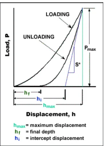
Figure 3.Typical load-displacement curve of the nanoindentation test.

The most commonly used method to obtain the hardness and the elastic modulus of a material by nanoindentation is the Oliver-Pharr method [25]. According to this method, the nanoindentation hardness as a function of the final penetration depth of indent can be determined by:

A P

H = max (2.1)

where Pmax is the maximum applied load measured at the maximum depth of penetration (hmax), A is the projected contact area between the indenter and the specimen. For a spherical indenter,

f Rh

A=2π (where R is the radius of the indenter), whereas for a pyramidal (Berkovich or Vickers) indenter, A can be expressed as a function of hfas

128 / 1 8 4

/ 1 3 2 / 1 2 1

2 504 .

24 h_f C h_f C h_f C h_f C h_f

A= + + + +_L+ (2.2)

where C1 to C8 are constants and can be determined by standard calibration procedure. The final

penetration depth, hf, can be determined from the following expression:

∗

− =

S P h

h_{f max} ε max (2.3)

where ε is a geometric constant, ε=0.75 for a pyramidal indenter, and ε=0.72 for a conical indenter. S* is the contact stiffness which can be determined as the slope of the unloading curve at the maximum loading point, i.e.

max

h h dh dP S

=

∗ _⎟

⎠ ⎞ ⎜ ⎝ ⎛

= (2.4)

A S Er

π β

2

∗

= (2.5)

where β is a constant that depends on the geometry of the indenter. For both a Berkovich and a Vicker’s indenter, β=1.034, whereas for both a conical and a spherical indenter, β=1. The specimen elastic modulus (Es) can then be calculated as:

i i

s s

r E E

E

2 2 ₁ 1

1 ₌ −υ ₊ −υ

(2.6)

Where E_i,_s and υi,s are the elastic modulus and Poisson’s ratio, respectively, for the indenter and the specimen. For a diamond indenter, Ei is 1140 GPa and υi is 0.07. The contact stiffness, S*, can be derived from the unloading curve which simply obeys the following power law

n

f h h B

P= ( − ) (2.7)

where B and n are empirical constants that can be determined by fitting the experimentally measured pairs of data (P, h) during unloading. Thus the contact stiffness can be expressed as

1

max )

( max

− =

∗ _{⎟ = −}

⎠ ⎞ ⎜ ⎝ ⎛

= n

f h

h

h h Bn dh

dP

S (2.8)

Therefore, the specimen’s hardness H and elastic modulus Es will be obtained from this set of equations.

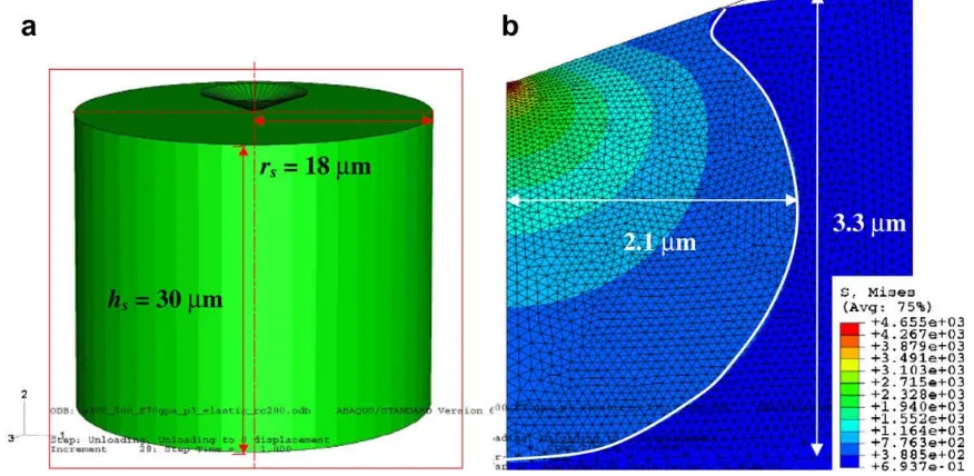
Figure 4. (a) Geometry of indentation of a cylindrical specimen with a conical indenter. (b) The Mises equivalent stress field in the specimen during indentation at hmax = 600 nm. (The stress values must be multiplied by 107 to respect the scale of the problem) [15].

2.2 Analytical Modeling Stiffness of Nanocomposites

[image:7.612.83.521.75.289.2]

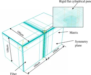
Figure 5. Illustration of a three dimensional nanoindentation finite element model [18].

[image:8.612.139.456.72.332.2]

In nanocomposites, there are typically three kinds of fillers. They are cylinder-like nanofibers (nanotubes), flake-like (disk-like) platelets (nanolayers, nanoclays), and spheroid-like particulates, refer to Figs. 1 and 2. For the fiber-reinforced nanocomposites, there are two cases depending on the orientation of the fibers, i.e. aligned fibers and randomly oriented fibers, see Fig. 6 below.

The popular micromechanical models for prediction of modulus of elasticity are summarized and discussed in the following:

2.2.1 Voigt upper bound and Reuss lower bound (V-R model)

Assumed aligned fibers, and fibers and matrix are subjected to the same uniform strain in the fiber direction, Voigt [74] got the effective modulus in the fiber direction as:

m f

L E E

E =φ +(1−φ) (2.9)

Reuss [75] applied the same uniform stress on the fiber and matrix in the transverse direction (normal to the fiber direction), and got the effective modulus in the transverse direction as:

m f

T E E

E

φ φ ₊ −

= 1

1

(2.10)

the longitudinal and transverse directions, respectively. Equation (2.9) is the parallel coupling formula, and it is also called the “rule of mixtures”, whereas (2.10) is the series coupling formula, and it is also called the “inverse rule of mixtures”.

a. Aligned fibers b. Randomly oriented fibers

c. Aligned platelets d. particulates

Figure 6. Schematics of nanocomposites: (a) with aligned fibers; (b) with randomly oriented fibers; (c) with aligned platelets; and (d) with randomly oriented particulates [6].

Equations (2.9) and (2.10) can be extended to any two-phase composites regardless the shape of the filler, and E_L and E_T represent the upper and lower bounds of the modulus of the composite, respectively. Note that in these formulas, only three parameters are involved, i.e. modulus of the fiber and the matrix, and the fiber volume fraction.

2.2.2 Hashin and Shtrikman upper and lower bounds (H-S model)

bulk moduli, Kupper and Klower, and shear moduli, Gupper and Glower, of the composite are given as: 1 4 3 3 1 ) 1 ( − ⎥ ⎥ ⎦ ⎤ ⎢ ⎢ ⎣ ⎡ + + − − + = f f f m f upper G K K K K

K φ φ (2.11)

1 4 3 ) 1 ( 3 1 − ⎥ ⎥ ⎦ ⎤ ⎢ ⎢ ⎣ ⎡ + − + − + = m m m f m lower G K K K K

K φ φ (2.12)

1 ) 4 3 ( 5 ) 2 ( 6 1 ) 1 ( − ⎥ ⎥ ⎦ ⎤ ⎢ ⎢ ⎣ ⎡ + + + − − + = f f f f f f m f upper G K G G K G G G

G φ φ (2.13)

1 ) 4 3 ( 5 ) 2 )( 1 ( 6 1 − ⎥ ⎥ ⎦ ⎤ ⎢ ⎢ ⎣ ⎡ + + − + − + = m m m m m m f m lower G K G G K G G G

G φ φ (2.14)

where the subscripts “f” and “m” refer to the filler (fiber) and matrix, respectively. The upper and lower bounds of the elastic modulus can then be calculated using the following relation:

G K K E / 3 1 9 +

= (2.15)

Similar to Voigt and Reuss models, H-S model only involves three parameters.

2.2.3 Halpin-Tsai model (H-T model)

For aligned fiber-reinforced composite materials, Halpin and Tsai [78-81] developed the equations for prediction of elastic constants based on the work of Hermans [82] and Hill [83]. The H-T model is a semi-empirical model, and the longitudinal and transverse moduli are given by: m L L L E d l E φη φη − + = 1 ) / ( 2 1 (2.16) m T T T E E φη φη − + = 1 2 1 (2.17)

where l and d are the length and diameter of the fiber, and η_L and η_T take the following expressions: m f m f L E d l E E E ) / ( 2 + − =

η (2.18)

m f m f T E E E E 2 + − =

η (2.19)

H-T model takes the consideration of the fiber geometry, and has five independent parameters.

2.2.4 Hui-Shia model (H-S model)

Mori and Tanaka [84] developed analytical expressions for elastic constants based on the equivalent inclusion model of Eshelby [85]. Taya and Mura [86] and Taya and Chou [87] used Mori-Tanaka approach to predict the longitudinal modulus of fiber-reinforced composites, Weng [88] and Tandon and Weng [89] further developed equations for the complete set of elastic constants of composite materials with aligned spheroidal isotropic inclusions. Based upon the results of Tandon and Weng [89], Hui and Shia [90] and Shia et al. [91] derived simplified formulas for predicting the overall moduli of composites with aligned reinforcements with emphases on fiber-like and flake-like reinforcements, and found that their theoretical predictions agree well with experimental results. The H-S model presents the Young’s modulus as follows:

1 1 − ⎥ ⎦ ⎤ ⎢ ⎣ ⎡ ₋ = ξ φ m L E

E (2.20)

1 3 1 ( 4 1 − ⎥ ⎦ ⎤ ⎢ ⎣ ⎡ Λ + + − = ξ ξ φ m T E

E (2.21)

where ⎥ ⎦ ⎤ ⎢ ⎣ ⎡ − − − − + − + = 1 2 / ) 1 ( ) 1 ( 3 ₂ 2 α α φ φ

ξ g g

E E

E

m f

m _(2.22)

⎥ ⎦ ⎤ ⎢ ⎣ ⎡ − − + − = Λ 1 2 ) 25 . 0 ( 3 ) 1 ( ₂ 2 2 α α α

φ g (2.23)

⎪ ⎪ ⎩ ⎪⎪ ⎨ ⎧ ≤ + − − − ≥ − − − = − − 1 ] cos 1 [ ) 1 ( 1 ] cosh 1 [ ) 1 ( 1 2 2 / 3 2 1 2 2 / 3 2 α α α α α α α α α α α α

g (2.24)

and α is the aspect ratio of the filler, defined as the ratio of the filler’s longitudinal (with Young’s modulus E_L) length to its transverse (with Young’s modulus E_T ) length. For example, refer to Fig. 2, α =l/d for nanotube, α =t/D for nanoplatelet, and E_L will be along axis 3, and E_T will be along axis 1 (or 2).

2.2.5 Wang-Pyrz model (W-P model)

the Eshelby tensor [85], thus are not final. Wang and Pyrz [94] further gave the closed and concise formulas for the overall bulk modulus and shear modulus as follows:

) 1 (

1 φ α

φϕ

− − +

=Km Km

K (2.25)

) 1 (

1 φ β

φψ μ

μ μ

− − +

= m m (2.26)

The expressions for ϕ, ψ , α and β are given in the Appendix.

Note that W-P model is based on the Mori-Tanaka approach, and deals with the composite materials reinforced with randomly oriented and transversely isotropic spheroids. By varying the aspect ratio, the oblate spheroids can be approximate to platelets, and the prolate spheroids can be approximate to fibers.

2.2.6 Cox model (Shear lag model)

Shear lag model was the first micro-mechanics model for fiber-reinforced composites. Cox [95] analyzed a single fiber of length l and radius r_f , which is encased in a concentric cylindrical shell of matrix having radius R. He derived the longitudinal modulus as

m f

L

L E E

E =η φ +(1−φ) (2.27)

where η_L is a length-dependent efficiency factor,

2 /

) 2 / tanh( 1

l l

L β

β

η = − (2.28)

with

) / ln( 4 2 2

φ μ β

R f f

m K E r

= (2.29)

R

K is a constant that depends on the fiber packing arrangements. For some typical fiber packing arrangements, the values of K_R are given in Table 1 [96].

Table 1. Values for K_R in Eq. (2.29) FIBER PACKING K_R

Cox _{2π/ 3=3.628}

Composite cylinders 1.000

Hexagonal _{π/2 3=0.907}

Square π/4=0.785

reinforcement in two directions, if appropriately oriented, while fibers provide primary reinforcement in one direction. If the longitudinal modulus E_L and the transverse modulus E_T are known, then the effective modulus of the composite with randomly oriented fibers and platelets in all three orthogonal directions are given by [97]:

T L

fiber

D E E

E3 =0.184 +0.816 (2.30)

T L

platelet

D E E

E3 =0.49 +0.51 (2.31)

2.3 Molecular Dynamics Simulation

In modeling mechanical properties of nanocomposites, there are two main approaches: one is molecular dynamics simulation using direct methods, and the other is finite element simulation using “continuum” methods. Molecular dynamics simulation is a technique that allows one to determining the physical and mechanical properties of materials in nanoscale through solving Newton’s equations of motion with the atoms interacting through assumed interatomistic potentials [98, 99]. It generates information such as atomic positions, velocities and forces from which some macroscopic properties can be derived by means of statistical mechanics. Molecular dynamics simulation usually consists of three constituents: (1) a set of initial conditions (e.g., initial positions and velocities of all particles in the system); (2) the interaction potentials to represent the forces among all the particles; (3) the evolution of the system in time by numerically solving a set of classical Newtonian equations of motion for all particles in the system [100]. In 1997, Cornwell et al. used molecular dynamics to predict the elastic properties of single-walled carbon nanotubes [101]. In recent years, molecular dynamics simulation has been extensively used in predicting mechanical properties of carbon nanotubes and nanotubes reinforced composites [102-109], graphite/epoxy nanocomposites [110-112], and other nanocomposites [113-119].

Molecular dynamics simulation involves the proper selection of interaction potentials, numerical integration, periodic boundary conditions, and the controls of pressure and temperature to mimic physically meaningful thermodynamic ensembles. The interaction potentials together with their parameters form a force field which describes in detail how the particles in a system interact with each other. Such a force field may be obtained by quantum method, empirical method or quantum-empirical method. The criteria for selecting a force field include the accuracy, transferability and computational speed. The total potential energy U may consist of a number of bonded and non-bonded interaction terms:

∑

+

∑

+

∑

+

∑

+

∑

−

= U_bond U_angle U_torsion U_inversion U_{non bonded}

U (2.32)

is bonded to other three, as shown in Fig. 7 [120]. The last term represents non-bonded interactions between two atoms. It usually includes van der Waals and electrostatic interactions.

Figure 7. Bond structures and corresponding energy terms of a graphene cell [120].

Molecular dynamics simulations can be performed in different ensembles, such as grand canonical (μVT), microcanonical (NVE), canonical (NVT) and isothermal–isobaric (NPT). The constant temperature and pressure can be controlled by adding an appropriate thermostat (e.g., Berendsen, Nose, Nose–Hoover and Nose–Poincare) and barostat (e.g., Andersen, Hoover and Berendsen), respectively. The software packages available for molecular dynamics simulations include DL-POLY developed by Daresbury Laboratory [121, 122], LAMMPS developed by Sandia National Laboratories [123], and TINKER developed by University of Washington [124].

Table 2. Functional form and parameters for the force field [125]

Interactio n

Potential Functional form Parameters

Bond Harmoni c 2 0) ( 2 1 )

(r k r r

U = r − r

k = 700 kcal/mol o

0 =1.53A

r

θ

k = 112.5 kcal/mol 0

0 =109.471 θ

φ

k = 1.00 kcal/mol, m=3

PE–PE:

ε = 0.113266kcal/mol o A 28 . 4 = σ PE–Bucky:

ε = 0.107290 kcal/mol o A 825 . 3 = σ o A 7 . 10 = cut r Angle Harmoni c cosine 2 0)] cos( ) [cos( 2 1 )

(θ = k_θ θ − θ

U Dihedral Cosine 2 )] cos( 1 [ 2 1 )

(φ kφ mφ

U = +

Non-bonded Lennard-Jones ⎪⎩ ⎪ ⎨ ⎧ ≥ < ⎥⎦ ⎤ ⎢⎣ ⎡ ₋ = cut cut r r r r r r r U 0 ) ( ) ( 4 )

( 12 6

σ σ

ε

[image:16.612.111.466.240.323.2]

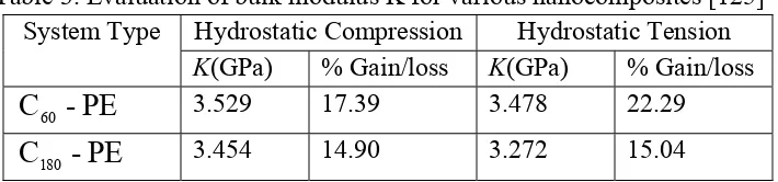
Fig. 8 shows the cells of different neat and nanocomposites model used for simulation. Periodic boundary conditions were employed to replicate the unit cells in three dimensions. Software package DL_PLOY (version 2.14) was used in the simulation. All the calculations were carried out at a temperature of 3000K with 0.5 fs time steps. Two major steps of simulation for both neat polymer and nanocomposites were performed. In the first step, the equilibrium state of the molecular model was obtained, and then the model was subjected to different strain fields and re-equilibrated. Adnan et al. applied a uniform strain field (0.5%) to the periodic cells of both neat polymer and nanocomposites. For the cases of hydrostatic tension and hydrostatic compression, they evaluated the bulk modulus K, and their results were shown in Table 3.

Table 3. Evaluation of bulk modulus K for various nanocomposites [125] System Type Hydrostatic Compression Hydrostatic Tension

K(GPa) % Gain/loss K(GPa) % Gain/loss

PE

-C

60 3.529 17.39 3.478 22.29

PE

-C

180 3.454 14.90 3.272 15.04

It is evident from Table 3 that elastic properties of nanocomposites are improved appreciably with the infusion of bucky-balls in PE matrix, and they are also significantly affected by the size of reinforcing bucky-balls.

2.4 Finite Element Modeling

As a very general and powerful numerical analysis tool, finite element method was used to predict mechanical properties of composite materials started in early 1970s [128-129]. Since then, various finite element models have been developed to characterize all kinds of composite materials [e.g. 130-136]. In 1991, Sumio Iijima, a Japanese scientist, discovered carbon nanotubes (CNTs) which possess exceptionally high stiffness and strength, as well as superior electrical and thermal properties [137-139]. Soon after that CNTs were used as reinforcement in developing nanocomposite materials. In the past decade or so, there have been explosively experimental work [e.g. 7, 8, 140-155] and analytical work [e.g. 156-169], as well as finite element modeling work [e.g. 170-198] on developing, analyzing and characterizing CNT reinforced nanocomposites and other nanocomposites. In the following, three finite element modeling approaches will be discussed. They are multiscale representative volume element (RVE) modeling, unit cell modeling, and object-oriented modeling.

2.4.1 Multiscale RVE modeling

nanoscale RVE based on elasticity theory and solved by the finite element method. An RVE is composed of a single (or multiple) nanofiller(s) with surrounding matrix material, plus proper boundary conditions to account for the effects of the surrounding materials. It is used as a building block to assemble the composite. Zhang et al. [201] linked continuum analysis with atomistic simulation by incorporating interatomic potential and atomic structures of CNTs directly into the constitutive law. Shi et al. [185] presented a hybrid atomistic/continuum mechanics method to study the deformation and fracture behavior of CNTs embedded in composites. The method is based on a representative unit cell divided into three distinct regions analyzed using an atomistic potential, a continuum method based on the Cachy–Born rule and a micromechanics method, respectively. Li and Chou [180] proposed a multi-scale modeling approach to study the compressive behavior of CNT/polymer composites. They modeled the nanotube at the atomistic scale and analyzed the matrix deformation using the continuum finite element method. The van der Waals interactions between carbon atoms and the finite element nodes of the matrix were simulated using truss rods.

The multiscale RVE integrates nanomechanics and continuum mechanics, thus bridging the length scales from the nano- through the mesoscale. The procedure of multiscale RVE modeling is exhibited by the work of Tserpes et al. [172] in the following. Tserpes et al. proposed a multiscale RVE to investigate the tensile behavior of CNT/polymer composites. The RVE is a rectangular solid whose entire volume is taken up by the matrix, and the nanotube is modeled as a three-dimensional (3D) elastic beam. The 3D solid elements and beam elements are used to model the matrix and nanotube, respectively. The RVE is synthesized in two steps. First, the behavior of the isolated nanotube is simulated using the progressive fracture model [202]. The concept of the model is based on the assumption that carbon nanotubes, when loaded, behave like space-frame structures. The bonds between carbon atoms are considered as load-carrying members while carbon atoms as joints of the members. The non-linear behavior of the C-C bonds is modeled by the modified Morse interatomic potential [203], and the nanotube structure is modeled by finite element method. Second, the nanotube is inserted into the matrix to form the RVE. The matrix is modeled by solid elements, and the nanotube is represented by 3D elastic beam elements created by binding the nodes of the matrix. The synthesis of the RVE is shown in Fig. 9.

2.4.2 Unit cell modeling

Figure 9. Synthesis of the RVE [172].

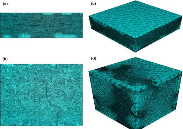
The most common method used to characterize the mechanical properties of nanocomposites with unit cell is the finite element method. Hbaieb et al. [177] examined the Young’s modulus of nanoclay/polymer nanocomposites with both 2D and 3D unit cells using the finite element method. Four unit cells were created. They are, respectively, 2D and 3D aligned and randomly oriented nanoclay particles models, as shown in Fig. 10. Two kinds of boundary conditions are considered. They are periodic boundary conditions and symmetrical boundary conditions. For the 2D models (both aligned and random cases) the periodic boundary conditions are:

u(RE)=u(LE)+

δ

₁ v(RE)=v(LE) u(TE)=u(BE) v(TE)=v(BE)+

δ

₂

where RE, LE, TE, BE and

δ

₁ and

δ

₂ are the right, left, top, bottom edges and the axial and transverse displacements, respectively. The symmetrical boundary conditions for the 2D models are:

where

δ

is the given normal displacement in the x direction. In addition, all edges are free of shear traction and the top edge is free of normal traction as well.

For the 3D models (both aligned and random cases) only symmetrical boundary conditions are applied, and they are given as:

u(LF)=0 v(BF)=0 w(BKF)=0 u(RF)=

δ

where LF, BF, BKF and RF stand for left face, bottom face, back face and right face. All other faces are free of any displacement or traction constraints. The numerical results indicated that 2D models do not predict the elastic modulus of clay/polymer nanocomposites accurately. The Mori-Tanaka model [89] gives reasonably accurate predictions of the stiffness of the nanocomposites whose volume fraction is less than 5% for aligned particles but underestimates the stiffness at higher volume fractions. For randomly oriented particles the W-P model [94] overestimates the stiffness of the nanocomposites.

[image:19.612.144.442.344.554.2]

Figure 10. Mesh details of the model for (a) 2D aligned particle distribution, (b) 2D randomly oriented-particle distribution, (c) 3D aligned particle distribution, and (d) 3D randomly oriented-particle distribution. Particle volume fraction is 5%, the particle aspect ratio is 50, Ep/Em=100, ν m=0.35, ν p=0.2. Subscripts p and m represent particle and matrix, respectively [177].

the unit cell are

10

×

20

×

20

μ

m

3 which contains (fully or partially) 260 whiskers. The volume fraction of the whiskers is 15%. Fig. 11 shows a typical unit cell (with the meshes of the whiskers) and an optical micrograph of the composite. For the Young’s modulus and overall elastic-plastic response of the composite, the finite element modeling results are in excellent agreement with the experimental results.

Figure 11. (a) 3D random whisker-reinforced composite model, and (b) an optical micrograph of squeeze-infiltrated Al18B4O33/Mg random whisker composite [170].

2.4.3 Object-oriented modeling

In both multiscale RVE modeling and unit cell modeling, two basic assumptions are made. First, nanofillers can be idealized to simple geometries such as spheres, ellipsoids, cylinders, or cubes. And second, nanocomposites can be reproduced by assembling a large number of such RVEs (or unit cells). This can be a serious limitation when dealing with complex and highly heterogeneous nanocomposites. For example, for highly variable and irregular angular structure of fillers, using approximation of simple geometrical particles could not capture the complex morphology, size, and spatial distribution of the reinforcement. Therefore, the object-oriented modeling which is able to capture the actual microstructure morphology of the nanocomposites becomes necessary in order to accurately predict the overall properties.

[8, 178, 179, 217]. In the following, a 2D object-oriented finite element modeling will be discussed, followed by a 3D modeling.

[image:21.612.150.474.135.389.2]

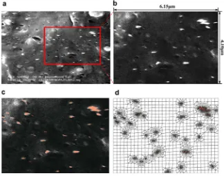
Figure 12. Typical example of creating OOF model of PP/organoclay nanocomposites (5 wt% in clay content): (a) original SEM image, (b) captured SEM image portion, (c) image segmentation using pixel selection, and (d) finite element mesh (highlighted regions contain organoclay particles and the rest are PP matrices) [8].

Dong et al. [8] studied the mechanical properties of polypropylene (PP)/organoclay nanocomposites with different clay contents ranging from 1 to 10 wt%. Their work started with the specimen fabrication through experimental characterization to theoretical predictions and numerical modeling using OOF. SEM micrographs from longitudinal loading direction of the specimen were captured and mapped onto the finite element model, as shown in Fig. 12. The actual nano/microstructures (their size, shape, and distribution etc.) of the PP and the organoclay were used in the computational model, and each phase was attributed the corresponding material properties. The OOF modeling results for the tensile modulus show a good agreement with the experimental data and theoretical predictions.

results of the Young’s modulus and the stress-strain relations from the object-oriented (microstructure-based) model with the results of the experiment and the numerical results from simplified models (which include rectangular prism, ellipsoids, and multiparticle-spheres, etc.). Some of the results were shown in Fig. 13. Their results indicate that 3D microstructure-based model can accurately predict the properties of particle-reinforced composites, while the simple analytical models can not as they do not account for the microstructural factors that influence the mechanical behavior of the material.

[image:22.612.136.429.208.483.2]

Figure 13. Comparison between 3D finite element models incorporating actual

microstructure and approximation to spherical particles: (a) FEM models, (b) von Mises stress distribution in particles, and (c) plastic strain in matrix [178].

3. MECHANICAL PROPERTY ENHANCEMENT

Fillers added to matrix can change the mechanical properties of the matrix material. Comparing to traditional composite materials, nanocomposites have the following characterizations:

1. Nanoparticles can substantially improve the mechanical properties of the host matrix materials [140,142,218-220]. Even at very low filler volume content such as 1-5%, a considerable improvement of the mechanical properties can be achieved [143, 221-223]. 2. It is observed that for some nanocomposites, with the same filler volume fraction, the

3. In general, the stiffness of nanocomposites tends to increase as the filler volume fraction increases. This function may be nonlinear. There may exist a critical volume fraction beyond which the stiffness starts decrease [228].

For conventional composite materials, micromechanics theories consider that the overall mechanical properties of composites are functions of constituent properties, constituent volume fraction, inclusion shapes and orientations, and state of dispersion. It does not consider the interactions between filler and matrix at their interface. For nanocomposites, the mechanical property enhancement not only depends on the above factors, but also depends on the interaction between the filler and the matrix.

3.1 Mechanisms of stiffness and strength enhancement

It is widely accepted that there is an interphase exist between the nanofillers and the matrix material in nanocomposites. This interphase is a transition region, which extends nanometers to micrometers over which the mechanical and physical properties change from the properties of filler to the properties of the matrix. Among many researchers who studied the nanocomposites interphase behavior, Boutaleb et al. [156] investigated the influence of interphase on the overall behavior of silica spherical nanoparticle/polymer composites by means of analytical and finite element methods. Fig. 14 shows a schematic of a composite material containing randomly located spherical nanoparticles (left) and a spherical nanoparticle coated with a graded interphase (right). The interphase is represented as a third phase around the nanoparticles. A model of axisymmetric RVE with periodical boundary conditions was examined. The analysis results show that the interphase is a dominant parameter controlling the overall nanocomposite behavior.

To estimate the elastic modulus of the interphase in polymer nanocomposites, Saber-Samandari and Khatibi [229] developed a 3D unit cell model to represent the three constituent phases including particle, interphase and matrix. The elastic modulus of the interphase at any point, r, is described by a power law as:

2 /

)

/

(

/

)

(

n

f i

i f i m f i

m i

r

r

r

r

r

r

E

E

r

r

E

r

E

_⎟

⎟

⎠

⎞

⎜

⎜

⎝

⎛

−

−

−

+

=

(3.1)

[image:24.612.79.483.69.242.2]

Figure 14. Schematic of a composite material containing randomly located spherical nanoparticles (left) and a spherical nanoparticle coated with an interphase (right) [156].

How exactly the interphase affects the nanocomposites properties is still a research topic. Some intend to think the interphase refined the grain size of matrix leads to smaller critical flaw size and higher strength. Some researchers believe that nanoparticles yield dislocations around them, and these dislocations release residual stresses in the matrix. Thus the defect size along the grain boundaries is reduced. There are also some researchers who think nanofillers impart additional strength of their own to the matrix through the interphase. Nevertheless to say, the strengthening mechanism of nanocomposites is not fully understood. Several mechanical properties of nanocomposites are also improved for the same reason, such as hardness, wear resistance, and thermal shock resistance.

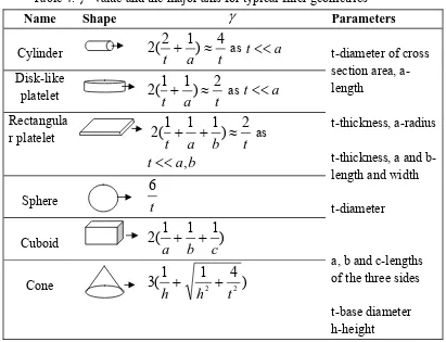
The interaction between nanofillers and matrix is the key to the nanocomposites properties enhancement. There are many factors affecting that interaction, such as the filler volume (weight) fraction, degree of dispersion, the filler geometry and orientation, etc. We assume the same volume fraction and identical degree of dispersion, only the filler geometry (aspect ratio) and orientation will be considered. We define a reactive surface area per unit volume of filler,γ , as

V

A

=

γ

(3.2)

where A and V are surface area and volume of the filler, respectively. Table 4 shows the major axis and the

γ

value for some typical geometry of the nanofillers.

[image:25.612.78.489.161.476.2]

thickness of the disk are the same. According to the values in Table 4, the reinforcement efficiency of the three geometries in the major axis direction, from good to poor, is sphere-cylinder-disk. But nanoplatelets are thought to possess better reinforcement effects than those of spherical and fiber-like particles [230].

Table 4. γ value and the major axis for typical filler geometries

Name Shape

γ

Parameters

Cylinder

_t

_a

_t

4

)

1

2

(

2

+

≈

as

t

<<

a

_{t-diameter of cross}

section area, a-length

t-thickness, a-radius

t-thickness, a and b-length and width

t-diameter

a, b and c-lengths of the three sides

t-base diameter h-height

Disk-like

platelet

2

(

1

_t

+

_a

1

)

≈

2

_t

as

t

<<

a

Rectangula

r platelet

2

(

1

_t

+

_a

1

+

_b

1

)

≈

2

_t

as

b

a

t

<<

,

Sphere

6

_t

Cuboid

)

1

1

1

(

2

c

b

a

+

+

Cone

3

(

1

1

2

4

2

)

t

h

h

+

+

As the filler orientation is very important in reinforcement, equation (3.2) has to be modified to account for the effect of orientation of the filler surfaces. Now we define an effective surface area per unit volume of filler,

γ

, as

V

A

=

γ

(3.3)

where

A

is the effective filler surface area, and it represents the portion of surfaces which is normal to the direction of major axis (see Table 4). The value of

γ

for sphere, disk, and cylinder in the major axis is 3/2t, 2/t, and 4/t, respectively. Therefore, in the major direction shown, the order of reinforcement efficiency, from good to poor, is cylinder-disk-sphere.

than that of nanocylinders. This is because sphere is isotropic, and disk is transversely isotropic, and cylinder is anisotropic.

For all the geometries of the filler, as the characteristic dimension (the smallest dimension) decreases, the value of

γ

will increase. That is, the smaller the filler, the better enhancement it will provide. This is similar to the Hall-Petch effect on the strength of metals. Hall-Petch relates the yield stress of a metal to its average grain diameter d as

2 / 1 0

−

+

=

kd

y

σ

σ

(3.4)

where

σ

₀ and

k

are the constants related to the material of interest. The yield stress increases as the grain size decreases. It is also interesting to note that just as Hall-Petch equation does not apply to extremely fine grain sizes, fine size filler enhancement on nanocomposites may also have a limit. Schiotz and Jacobsen [231] investigated nanocrystalline copper, and pointed out that there may be a maximum in the strengthening that can be obtained by decreasing the grain size, so that below a certain critical grain size the strength begins to decrease again as the grain size decreases.

3.2 Fracture Toughness

Nanocomposites can not only improve stiffness and strength, but also fracture toughness [232-242]. In general, the fracture toughness of nanocomposites increases as the volume fraction increases, and increases as the nanofiller size decreases. For silica/epoxy nanocomposites, Ragosta et al. [235] found the fracture toughness improved as the volume fraction of 15-nm silica particles increases. Similar results were obtained by Zhang et al. [234] with 25-nm silica particles, and by Chen et al. [232] with 12-nm silica particles. Through experiments and an analytical model, Adachi et al. [233] studied the mode I fracture toughness of silica/epoxy nanocomposites, and found that the toughness increased drastically as the silica volume fraction increased and the particle diameters decreased. In nanocomposites with a low volume fraction of particles, the volume fraction affected the fracture toughness more; and with high volume fractions, the particle size affected the fracture toughness more.

propagating crack tip (Fig. 15B). The highly stressed frontal process zone (FPZ) ahead of the crack tip is then released by nano-crack nucleation, and the nano-cracks expand the FPZ size, enhancing the fracture toughness of the materials [236].

[image:27.612.118.460.151.371.2]

Figure 15. Schematic description of the toughening mechanism in nanocomposites. (A) Intra-type nano-structure, (B) FPZ creation [244].

4.CONCLUDING REMARKS

Characterizing and modeling mechanical properties of nanocomposites is reviewed and evaluated. Nanocomposites are made by dispersing nanofillers (e.g., silicate and ceramic nanoparticles, CNTs, etc.) into matrix (e.g., some polymers, ceramics, metals, etc.). Comparing with conventional composite materials, nanocomposites have numerous advantages such as high mechanical and physical properties, and high reinforcement efficiency. The high enhancement of mechanical properties of nanocomposites is mainly attributed to the interaction between the nanofillers and the matrix material through the interphase which is a transition region from the nanofillers to the matrix, and the high value of the reactive surface area per unit volume of nanofillers.

developed to study nanocomposites. These techniques represent approaches at various time and length scales from molecular scale to microscale, and then to macroscale, and have shown success to various degrees in addressing many aspects of nanocomposites. The simulation techniques developed thus far have different strengths and weaknesses, depending on the need of research. Despite substantial progress made in the past decade, there are a number of challenges in computer modeling and simulation. New concepts, theories and computational tools should be developed. In general, there are two fronts that should be pointed out. First, there is a need to develop new and improved simulation techniques at individual time and length scales. Secondly, it is important to integrate the developed methods at wider range of time and length scales, spanning from quantum domain to molecular domain, to mesoscopic domain, and finally to macroscopic domain, to form a useful tool for exploring the structural and mechanical properties, as well as optimizing design of nanocomposites [100]. Specific challenges and the solution strategies are discussed in the following:

1. In either developing new or characterizing the current exist nanocomposites, a comprehensive approach should be adopted that integrates the experimental techniques with nanomechanics-based analytical explorations and computer modeling and simulation.

2. New computational tools are specially needed in the area of multiscale RVE modeling. The multiscale RVE modeling is in nature a “local-global” approach. In order to catch the local nano/micro characteristics, quantum mechanics or molecular dynamics needs to be explored. But the prediction of global macro-mechanical properties requires the continuum mechanics-based finite element method. How to transit from local to global becomes a research issue. Ogata et al. [198] proposed a way of combing quantum mechanics, molecular dynamics, and finite elements. In regions where the atoms obey the laws of continuum mechanics, the finite element method is used. However, in critical areas such as the extremity of a fracture, molecular dynamics and even quantum mechanics are required to obtain a more detailed study of the fracture process. The transition from the global to local levels involves a change of scale. Xiao and Belytschko [245] proposed a way of improving the numerical compatibility between regions modeled by molecular dynamics and those modeled using the finite element method. The suggested method is introducing a broad transition region by superposing the finite element mesh of the continuum region on the atomistic structure of the molecular dynamics region. Clearly, there is still a lot of work needs to be done in connecting the local parameters to the global parameters.

ACKNOWLEDGEMENTS

This work was supported by the funding from the Air Force Office of Scientific Research and the Department of Defense Research & Engineering Office with grant number FA9550-08-1-0230. The first two authors would also like to acknowledge the significant interaction and support from Drs. Jennifer Stewart-Wright and Evelyn Maria Thompson from Tennessee State University.

APPENDIX

Formulas Related to the Overall Moduli:

2 1 3 1 F F T_iijj = = α ) 2 2 ( 5 1 ) 3 1 ( 5 1 2 1 5 4 3 F F F F F T

T_ijij − _iijj = + + − = β ) 3 6 2 ( 3 1 2 7 2 7 1 6 1 6 2 B F A F B F A F

F + + +

= ϕ 5 ) ( 5 2 ) 2 ( 5 1 3 4 4 3 2 7 1 6 2 9 1 8 2 ϕ

ψ = + + + + + −

F A F A B F B F A F A F F where ) )( 2 3 )( 4 3 ( 3 1 )] 2 ( ) 3 2 )( 1 [( 3 1 )] 1 ( 2 ) 4 9 3 )( 1 ( 2 1 [ 3 1 1 2 1 2 1 1 B B R A R f R A R f R F − − − + − + + − + − + − + − + = θ θ θ θ ) 2 )]( 2 ( )[ 4 3 ( 2 1 ] ) 1 ( )[ 4 3 ( )] 1 ( ) 1 )( 1 [( ) 3 )( 1 ( 2 1 1 2 1 2 1 2 1 2 2 1 2 1 2 A B B A A A f R f R B B R A R f R A f R F + + + − − + − + − + − + − + + − + + − + = θ θ θ θ θ θ θ 4

3 ) ( )]

2 3 ( 1 [

1 f R f A

F = + − + θ + +θ

3 4 1 0.25[f 3 ) R( f)]A F = + + θ + θ −

] ) 1 ( )[ 4 3 ( )] 1 ( ) 1 )( 1 [( ) 3 )( 1 ( 2 1

2 _{1 2 1 2}

5 R f A R f R A R B B

F = + − + θ + − + + −θ + − θ + −θ

2 2

6 (3 4 )(2 3 )

2 1 )] 2 ( ) 3 2 )( 1 [( 2 1

1 R f R A R B

F = + − + + −θ + − − θ

1 1

7 [(1 )(3 9 4) 4 (1 )] (3 4 )(3 2) 2

1

1 R f R A R B

F = + − + θ − + −θ + − θ −

2 2

8 1 [(1 R)(1 f) R(1 )]A (3 4R)(1 )B

1 1

9 (1 )( 3 ) (3 4 )

2 1

1 R f A R B

F = + − + θ +θ −

The constants R, A_i(i =1, 2, 3, 4) and B_i (i =1, 2) are non-dimensional ones related to the elastic constants of the isotropic matrix and the transversely isotropic inhomogeneity.

m m m K R μ μ 4 3 3 + = 1 1 − − = m f f l k A

μ , m

f f l n A μ 2 2 −

= , ₃ = −1 m

f m A

μ , 4 = −1 m f p A μ m f f m f

f k l

K l k B μ 6 2 2 9 2 1 − − + = , m f f m f

f n l

K l n B μ 6 9 2 2 − − + =

where k, n, m, p, and l are the notations adopted by Hill. They can be expressed in general by stiffness tensor components as

) ( 2 1 2233 2222 C C

k = + , n=C₁₁₁₁, ( )

2 1

2233 2222 C C

m= − , p=C₁₂₁₂, l =C₁₁₂₂ For an isotropic material, the above constants degenerate into

μ

3 1

+ =K

k , μ

3 4

+ =K

n , m= p=μ, μ 3 2

− = K l

f and θ are related to the geometry of the spheroidal inhomogeneity, which are

spheroid, prolate for 1 / ), 3 2 ( 1 spheroid, oblate for 1 / ), 2 3 ( 1 3 2 1 2 2 1 3 2 2 2 ⎪ ⎪ ⎩ ⎪⎪ ⎨ ⎧ = = < = > = − − = > = = < = − − = c a a a a a c c a a a a a c f χ θ χ χ χ θ χ χ spheroid prolate for } cosh ) 1 ( { ) 1 ( spheroid oblate for } ) 1 ( {cos ) 1 ( 1 2 / 1 2 2 / 3 2 2 / 1 2 1 2 / 3 2 ⎪ ⎪ ⎩ ⎪⎪ ⎨ ⎧ − − − − − − = − − χ χ χ χ χ χ χ χ χ χ θ REFERENCES

[1] Braun T, Schubert A, Zsindely S. Nanoscience and nanotechnology on the balance. Scientometrics 1997;38:321–325.

[2] Alexandre M, Dubois P. Polymer-layered silicate nanocomposites: preparation, properties and uses of a new class of materials. Mater Sci Eng 2000;28:1–63.

[4] Kumar AP, Depan D, Tomer NS, Singh RP. Nanoscale particles for polymer degradation and stabilization-Trends and future perspectives. Progress in Polymer Science, 2009; 34: 479-515.

[5] Vaia RA,Wagner HD. Framework for nanocomposites. Mater Today 2004;7:32–7.

[6] Liu H, Brinson LC. Reinforcing efficiency of nanoparticles: A simple comparison for polymer nanocomposites. Compos Sci Technol 2008; 68: 1502-1512.

[7] Thilly L, Petegem SV, Renault PO, Lecouturier F, Vidal V, Schmitt B, Swygenhoven V. A new criterion for elastio-plastic transition in nanomaterials: Application to size and composite effects on Cu-Nb nanocomposite wires. Acta Materialia 2009; 57: 3157-3169. [8] Dong Y, Bhattacharyya D, Hunter, PJ. Experiental Characterisation and object-oriented

finite element modeling of polypropylene/organoclay nanocomposites. Comp Sci Technol 2008; 68: 2864-2875.

[9] Chen Q, Chasiotis I, Chen C, Roy A. Nanoscale and effective mechanical behavior and fracture of silica nanocomposites. Comp Sci Technol. 2008; 68: 3137-3144.

[10] Chen WH, Cheng HC, Hsu YC, Uang RH, Hsu JS. Mechanical material characterization of Co nanowires and their nanocomposite. Comp Sci Technol 2008; 68: 3388-3395.

[11] Song SY, Youn JR. Modelling of effective elastic properties of polymer based carbon nanotube composites. Polymer 2006; 47, 1741-1748.

[12] Schuster, BE, Wei Q, Ervin MH, Hruszkewycz SO, Miller MK, Hufnagel TC, Ramesh KT. Bulk and microscale compressive properties of a pd-based metallic glass. Scripta Materialia 2007; 57 (6), 517-520.

[13] Zhang H, Schuster BE, Wei Q, Ramesh KT. The design of accurate micro-compression experiments. Scripta Materialia 2006, 54(2), 181-186.

[14] Chang NK, Lin YS, Chen CY, Chang SH. Size effect of indenter on determining modulus of nanowires using nanoindentation technique. Thin Solid Films 2009; 517: 3695-3697. [15] Poon B, Rittel D, Ravichandran D. An analysis of nanoindentation in linearly elastic solids.

Int. J. Solids Struct. 2008; 45: 6018-6033.

[16] Han CF, Lin JF. Modeling to evaluate the contact areas of hard materials during the nano-indentation tests. Sensors Actuators A 2008; 147(1): 229-241.

[17] Ling Z, Hou J. A nanoindentation analysis of the effects of microstructures on elastic properties of Al2O3/SiC composites. Comp. Sci. Technol. 2007; 67: 3121-3129.

[18] Lee SH, Wang S, Pharr GM, Xu H. Evaluation of interphase properties in a cellulose fiber-reinforced polypropylene composite by nanoindentation and finite element analysis. Composites: Part A 2007; 38: 1517-1524.

[19] Qi HJ, Teo KBK, Lau KKS, Boyce MC, Milne WI, Robertson J, Gleason KK. Determination of mechanical properties of carbon nanotubes and vertically aligned carbon nanotube forests using nanoindentation. J. Mech. Phy. Solids. 2003; 51: 2213-2237.

[21] Gao SL, Mader E. Characterisation of interphase nanoscale property variations in glass fiber reinforced polypropylene and epoxy resin composites. Composites: Part A 2002; 33:559–576.

[22] Hodzic A, Stachurskia ZH, Kim JK. Nano-indentation of polymer–glass interfaces part I experimental and mechanical analysis. Polymer 2000;41:6895–905.

[23] Downing TD, Kumar R, Cross WM, Kjerengtroen L, Kellar JJ. Determining the interphase thickness and properties in polymer matrix composites using phase imaging atomic force microscopy and nanoindentation. J Adhes Sci Technol 2000;14:1801–12.

[24] Munz M, Sturm H, Schulz E, Hinrichsen G. The scanning force microscope as a tool for the detection of local mechanical properties within the interphase of fiber reinforced polymers. Composites: Part A 1998; 29A:1251–9.

[25] Oliver WC, Pharr GM. An improved technique for determining hardness and elastic modulus using load and displacement sensing indentation experiments. J Mater Res 1992; 7(6):1564–83.

[26] Fong H, Sarıkaya M, White SN, Snead ML. Nanomechanical properties profiles across dentin—enamel junction of human incisor teeth, Mater. Sci. Eng. 2000; C7: 119—128. [27] Zysset PK, Guo XE, Hoffler CE, Moore KE, Goldstein SA. Elastic modulus and hardness

of cortical and trabecular bone lamellae measured by nanoindentation in the human femur, J. Biomech. 1999; 32: 1005—1012.

[28] Habelitz S, Marshall GW, Balooch M, Marshall SJ. Nanoindentation and storage of teeth, J. Biomech. 2002; 35: 995—998.

[29] Cuy JL, Mann AB, Livi KJ, Teaford MF, Weihs TP. Nanoindentation mapping of the mechanical properties of human molar tooth enamel. Arch. Oral Biol. 2002; 47: 281—291. [30] Marshall GW, Balooch M, Gallagher RR, Gansky SA, Marshall SJ. Mechanical properties

of the dentinoenamel junction: AFM studies of nanohardness, elastic modulus, and fracture. J. Biomedic. Res. 2001; 54: 87—95.

[31] Poolthong S, Mori T, Swain MV. Determination of elastic modulus of dentin by small spherical diamond indenters. J. Dent. Mater. 2001; 20: 227—236.

[32] Habelitz S, Marshall SJ, Marshall GW, Balooch M. Mechanical properties of human dental enamel on the nanometer scale. Arch. Oral Biol. 2001; 46: 173—183.

[33] Xu HHK, Smith DT, Jahanmir S, Romberg E, Kelly JR, Thompson VP, Rekow ED. Indentation damage and mechanical properties of human enamel and dentin. J. Dent. Res. 1998; 77: 472—480.

[34] Kinney JH, Balooch M, Marshall SJ, Marshall GW, Wehs TP. Atomic force microscope measurements of the hardness and elasticity of peritubular and intertubular human dentin. J. Biomech. Eng. 1996; 118: 133—135.

[36] Kinney JH, Balooch M, Marshall SJ, Marshall GW, Weihs TP. Hardness and Young’s modulus of peritubular and intertubular dentine. Arch. Oral Biol. 1996; 41: 9-13.

[37] van Meerbeek B, Willems G, Celis JP, Roos JR, Braem M, Lambrechts P, Vanherle G. Assessment by nanoindentation of the hardness and elasticity of the resin—dentin bonding area. J. Dent. Res. 1993; 72: 1434—1442.

[38] Toparli M, Koksal NS. Hardness and yield strength of dentin from simulated nano-indentation tests. Comp Meth Progr Biomedi 2005; 77, 253-257.

[39] Shin C, Jin HH, Kim MW. Evaluation of the depth-dependent yield strength of a nanoindented ion-irradiated Fe–Cr model alloy by using a finite element modeling. J. Nucl. Mater. 2009; 392(3): 476-481.

[40] Li B, Gu YD, English R, Rothwell G, Ren XJ. Characterisation of nonlinear material parameters of foams based on indentation tests. Mater. Design 2009; 30(7): 2708-2714. [41] Wang, T.H., Fang, T.H., Lin, Y.C. A numerical study of factors affecting the

characterization of nanoindentation on silicon. Mater. Sci. Eng. 2006; 447: 244–253.

[42] Pelletier H, Krier J, Mille P. Characterization of mechanical properties of thin films using nanoindentation test. Mech. Mater. 2006; 38: 1182-1198.

[43] Yu, N., Polycarpou, A.A., Conry, T.F. Tip-radius effect in finite element modeling of sub-50 Nm shallow nanoindentation. Thin Solid Films 2004; 4sub-50, 295–303.

[44] Dao M, Chollacoop N, Vliet KJV, Venkatesh TA, Suresh S. Computational modeling of the forward and reverse problems in instrumented sharp indentation. Acta Mater. 2001; 49, 3899–3918.

[45] Zhang W, Subhash G. Finite element analysis of interacting Vickers indentations on brittle materials. Acta Mater. 2001; 49 (15): 2961-2974.

[46] Zhang W, Subhash G. An elastic–plastic-cracking model for finite element analysis of indentation cracking in brittle materials. Int. J. Solids Struct. 2001; 38(34/35): 5893-5913. [47] Lichinchi, M., Lenardi, C., Haupta, J., Vitalib, R. Simulation of Berkovich nanoindentation

experiments on thin films using finite element method. Thin Solid Films 1998; 312: 240– 248.

[48] Gan L, Ben-Nissan B. The effects of mechanical properties of thin films on nano-indentation data: Finite element analysis. Comp. Mater. Sci. 1997; 8: 273-281.

[49] Zeng K, Giannakopoulos AE, Rowcliffe DJ. Vickers indentations in glass—II. Comparison of finite element analysis and experiments. Acta Metallur. Mater. 1995; 43: 1945-1954. [50] Kral ER, Komvopoulos K, Bogy DB. Elastic–plastic finite element analysis of repeated

indentation of a half-space by a rigid sphere. J. Appl. Mech. 1993; 75: 829–841.

[51] Wang HF, Yang X, Bangert H, Torzicky P, Wen L. Two-dimensional finite element method simulation of Vickers indentation of hardness measurements on TiN-coated steel. Thin Solid Films 1992; 214: 68-73.

tensile yield strength of super- and ultrahard nanocomposites. Surf. Coat. Technol. 2009; 203: 3385-3391.

[53] Jiang W, Batra RC. Identification of elastic constants of FCC metals from 2D load-indentation curves. Comp. Mater. Sci. 2009; 45(2): 511-515.

[54] Harsono E, Swaddiwudhipong S, Liu ZS. Material characterization based on simulated spherical-Berkovich indentation tests. Scrip. Mater. 2009; 60(11): 972-975.

[55] Geng K, Yang F, Grulke EA. Nanoindentation of submicron polymeric coating systems. Mater. Sci. Eng. A. 2008; 479(1/2): 157-163.

[56] Farrissey LM, McHugh PE. Determination of elastic and plastic material properties using indentation: Development of method and application to a thin surface coating. Mater. Sci. Eng A 2005; 399: 254-266.

[57] Zeng K, Soderlund E, Giannakopoulos AE, Rowcliffe DJ. Controlled indentations: a general approach to determine mechanical properties of brittle materials. Acta Mater. 1996; 44: 1127-1141.

[58] Yoshino M, Aoki T, Chandrasekaran N, Shirakashi T, Komanduri R. Finite element simulation of plane strain plastic–elastic indentation on single-crystal silicon. Int. J. Mech. Sci. 2001; 43 (2): 313-333.

[59] Fisher FT, Brinson LC. Nanomechanics of nanoreinforced polymers. In: Rieth M, Schommers W, editors. Handbook of theoretical and computational nanoscience. American Scientific Publishers; 2006. 253–360.

[60] Moniruzzaman M, Winey KI. Polymer nanocomposites containing carbon nanotubes. Macromolecules 2006;39(16):5194–5205.

[61] Thostenson ET, Li CY, Chou TW. Nanocomposites in context. Compos Sci Technol 2005;65: 491–516.

[62] Ajayan PM, Schadler LS, Braun PV. Nanocomposite science and technology. Weinheim: WILEY-VCH Verlag GmbH & Co. KGaA; 2003.

[63] Srivastava D, Wei CY, Cho K. Nanomechanics of carbon nanotubes and composites. Appl Mech Rev 2003; 56: 215–30.

[64] Leamy MJ. Bulk dynamic response modeling of carbon nanotubes using an intrinsic finite element formulation incorporating interatomic potentials. Int J Solids Struct 2007; 44: 874– 94.

[65] Odegard GM, Gates TS. Modeling and testing of the viscoelastic properties of a graphite nanoplatelet/epoxy composite. J Intell Mater Syst Struct 2006;17: 239–46.

[66] Sears A, Batra RC. Buckling of multiwalled carbon nanotubes under axial compression. Phys Rev B 2006; 73:085410-1–085410-11.

[67] Arroyo M, Belytschko T. Continuum mechanics modeling and simulation of carbon nanotubes. Meccanica 2005;40(4–6):455–69.

[69] Arroyo M, Belytschko T. Finite element methods for the non-linear mechanics of crystalline sheets and nanotubes. Int J Numer Methods Eng 2004;59(3):419–56.

[70] Zhu LJ, Narh KA. Numerical simulation of the tensile modulus of nanoclay-filled polymer composites. J Polym Sci 2004; 42: 2391–406.

[71] Wu YP, Jia QX, Yu DS, Zhang LQ. Modeling Young’s modulus of rubber–clay using composite theories. Polym Testing 2004; 23: 903–9.

[72] Luo J-J, Daniel IM. Characterization and modeling of mechanical behaviour of polymer/clay nanocomposites. Compos Sci Technol 2003;63:1607–16.

[73] Fornes TD, Paul DR. Modeling properties of nylon 6/clay nanocomposites using composite theories. Polymer 2003;44:4993–5013.

[74] Voigt W. Uber die beziehung zwischen den beiden elasticitatsconstanten isotroper korper. Ann Phys 1889; 38:573–87.

[75] Reuss A. Berechnung der fliebgrenze von mischkristalen auf grund der plastizitatsbedingung fur einkristalle. ZAMM 1929; 9:49–58.

[76] Hashin Z, Shtrikman, S. A variational approach to the theory of the elastic behavior of multiphase materials. J Mech Phys Solids 1963; 11: 127-40.

[77] Hashin Z, Analysis of composite materials-a survey. J. Appl. Mech. 1983; 50: 481-505. [78] Halpin JC. Primer on composite materials: analysis. Lancaster: Technomic Publishing

Company; 1984.

[79] Halpin JC, Kardos JL. The Halpin-Tsai equations: a review. Polym Eng Sci 1976; 16: 344-52.

[80] Halpin JC. Stiffness and expansion estimates for oriented short fiber composites. J Compos Mater 1969; 3:742-4.

[81] Halpin JC, Tsai SW. Effect of environmental factors on composite materials; Air Force Technical Report AFML-TR 67-423. Dayton, OH: Wright Aeronautical Laboratories; 1967.

[82] Hermans JJ. The elastic properties of fiber oriented materials when the fibers are aligned. Proc Kon Ned Akad v Wetensch B 1967; 65: 1-9.

[83] Hill R. Theory of mechanical properties of fibre-strengthened materials: I elastic behaviour. J Mech Phys Solids 1964; 12: 199-212.

[84] Mori T, Tanaka K. Average stress in matrix and average elastic energy of materials with misfitting inclusions. Acta Metall 1973; 21:571–4.

[85] Eshelby JD. The determination of the elastic field of an ellipsoidal inclusion and related problems. Proc R Soc London A 1957; 241:376–96.

[86] Taya M, Mura T. On stiffness and strength of an aligned short-fiber reinforced composite containing fiber-end cracks inder uniaxial applied stress. J Appl Mech 1981; 48: 361-7. [87] Taya M, Chou T-W. On two kinds of ellipsoidal inhomogeneities in an infinite elastic

body: an application to a hybrid composite. Int J Solids Struct 1981; 17: 553-63.

[89] Tandon GP, Weng GJ. The effect of aspect ratio of inclusions on the elastic properties of unidirectionally aligned composites. Polym Compos 1984;5:327–33.

[90] Hui CY, Shia D. Simple formulae for the effective moduli of unidirectional aligned composites. Polym Eng Sci 1998;38:774–82.

[91] Shia D, Hui CY, Burnside SD, Giannelis EP. An interface model for the prediction of Young’s modulus of layered silicate-elastomer nanocomposites. Polym Compos 1998;19:608–17.

[92] Qiu YP, Weng GJ. On the application of Mori-Tanaka’s theory involving transversely isotropic spheroidal inclusions. Int J Eng Sci 1990; 28: 1121-37.

[93] Chen T, Dvorak GJ, Benveniste Y. Mori-Tanaka estimate of the overall elastic moduli of certain composite materials. J Appl Mech 1992; 59: 539-46.

[94] Wang J, Pyrz R. Prediction of the overall moduli of layered silicate-reinforced nanocomposites-part I: basic theory and formulas. Compos Sci Tech 2004;64:925-934. [95] Cox HL. The elasticity and strength of paper and other fibrous materials. Brit J Appl Phys

1952; 3: 72-9.

[96] Tucker III CL, Liang E. Stiffness prediction for unidirectional short-fiber composites: Review and evaluation. Compos Sci Tech 1999; 59: 655-671.

[97] Van Es M, Xiqiao F, Van Turnhout, Van der Giessen E. Comparing polymer-clay nanocomposites with conventional composites using composite modeling. In: Al-Malaika S, Golovoy AW, editors. Specially polymer additives: principles and applications. CA Malden, MA: Blackwell Science; 2001. Chapter 21.

[98] Rapaport DC. The Art and Science of Molecular Dynamics Simulation. Cambridge: Cambridge University Press; 2004.

[99] Frenkel D, Smit B. Understanding molecular simulation: from algorithms to applications. 2nd ed. San Diego: Academic Press; 2002.

[100] Zeng QH, Yu AB, Lu GQ. Multiscale modeling and simulation of polymer nanocomposites. Prog. Polym. Sci. 2008; 33: 191–269

[101] Cornwell CF, Wille LT. Elastic properties of single-walled carbon nanotubes in compression. Solid State Commun 1997;101:555–8.

[102] Zhu R, Pan E, Roy AK. Molecular dynamics study of the stress-strain behavior of carbon-nanotube reinforced Epon 862 composites. Mater Sci Eng A 2007; 447: 51-57.

[103] Mokashi VV, Qian D, Liu YJ. A study on the tensile response and fracture in carbon nanotube-based composites using molecular mechanics. Compos Sci Technol

2007;67:530–40.

[104] Zheng QB, Xue QZ, Yan KO, Hao LZ, Li Q, Gao XL. Investigation of molecular interactions between SWNT and polyethylene/polypropylene/polystyrene/ polyaniline molecules. J Phys Chem C 2007;111:4628–35.