To the Complete Set of Equations for a Static Problem of General Relativity

(1)

ISSN Online: 2153-120X ISSN Print: 2153-1196

DOI: 10.4236/jmp.2019.1012093 Oct. 29, 2019 1401 Journal of Modern Physics

To the Complete Set of Equations for a Static

Problem of General Relativity

Valery V. Vasiliev, Leonid V. Fedorov

Institute of Problems in Mechanics, Russian Academy of Sciences, Moscow, Russia

Abstract

The paper is concerned with the formulation of the static problem of general relativity. As known, this problem is reduced to ten equations for the com-ponents of the Einstein tensor and the solution of these equations is asso-ciated with two principal problems. First, since the components of the Eins-tein tensor identically satisfy four conservation equations, only six of these equations are mutually independent. So, the set of the Einstein equations ac-tually contains six independent equations for ten components of the metric tensor and should be supplemented with four additional equations which are missing in the original theory. Second, for a deformable solid the Einstein tensor is associated with the energy tensor which is expressed in terms of six stresses induced by gravitation. These stresses are not known and the relativ-ity theory does not propose any equations for them. Thus, the static problem of general relativity cannot be properly formulated because the set of govern-ing equations is not complete. In the paper, the problem of completeness of the general relativity governing set of equations is analyzed in application to the spherically symmetric static problem and the proposed approach is fur-ther described for the general case. As an example, linearized axisymmetric problem is considered.

Keywords

General Relativity, Coordinate Conditions, Compatibility Stress Equations, Spherically Symmetric Problem

1. Introduction. General Relativity Equations

The Einstein equation which specifies the Einstein tensor has the following form:

1 2

j j j

i i i

E =R − δ R_,

(

i j, =1,2,3,4

)

₍₁₎ How to cite this paper: Vasiliev, V.V. and

Fedorov, L.V. (2019) To the Complete Set of Equations for a Static Problem of Gener-al Relativity. Journal of Modern Physics, 10, 1401-1415.

https://doi.org/10.4236/jmp.2019.1012093

Received: September 16, 2019 Accepted: October 26, 2019 Published: October 29, 2019

http://creativecommons.org/licenses/by/4.0/

(2)

DOI: 10.4236/jmp.2019.1012093 1402 Journal of Modern Physics

in which j i

R ( i

i

R R= _{) are the components of the Ricci curvature tensor (we}

use mixed components because for the spherically symmetric problem consi-dered further they coincide with the physical components). The Einstein tensor is associated with the energy tensor as

j j

i i

E =χT ₍₂₎

where

4

8 G c

χ = π ₍₃₎

is the relativity gravitational constant expressed in terms of the classical constant G and the velocity of light c. The energy tensor expressed with the aid of Equa-tion (1) and EquaEqua-tion (2) identically satisfies the conservaEqua-tion equaEqua-tions

, 0

k i k

T = ₍₄₎

For the static problem,

j j

i i

T =σ _, 4 ₀

i

T =

(

i j, =1,2,3

)

_, 4 2 4

T =µc ₍₅₎

where j i

σ _{is the stress tensor and} µ_{is the density.}

Consider two problems associated with the formulation of the general relativ-ity static problem. First, substituting Equations (2) in Equation (1), we arrive at ten equations for ten components of the metric tensor in four-dimensional Rie-mannian space. However, the right parts of these equations identically satisfy Equations (4) which means that only six of ten Equation (1) are mutually inde-pendent. Thus, we have six equations for ten unknown functions. The additional equations which are usually referred to as coordinate conditions should be im-posed on the metric tensor. As known, the metric tensor of the Euclidean space must satisfy the Lame equations. Such equations do not exist for the Riemannian space. However, we can suppose that the Riemannian space induced by gravita-tion cannot be arbitrary and must be somehow restricted, e.g., by coordinate conditions. The necessity of such conditions was first mentioned by D. Hilbert

[1]. By now the widely recognized general form of these conditions has not been proposed. Existing particular conditions are discussed further in application to the spherically symmetric problem.

Second, changing E to T and then to σ _{in Equations (1), we arrive at the set}

of equations containing stresses on the left sides. These stresses are not known. Traditionally, Equation (1) is used to study the gravitation in the empty space for which j 0

i

T = _{and Equation (1) are homogeneous. For solids the stresses}

are not zero and the equations cannot be solved. The solution can be obtained if the solid is simulated with perfect fluid. In this case the nonzero stresses

1 2 3

1 2 3 p

σ =σ =σ = − _{, where}_p_{is the pressure that can be found from the}

(3)

al-DOI: 10.4236/jmp.2019.1012093 1403 Journal of Modern Physics

low us to express the stresses in terms of stress functions and to satisfy the equi-librium equations. Thus, the metric tensor of general relativity is analogous to the tensor of stress functions in theory of elasticity. In this theory, the stress functions are found from the compatibility equations which postulate that the geometry of the stressed solid is Euclidean. In general relativity, the geometry is Riemannian and the compatibility equations of the theory of elasticity cannot be directly applied.

Thus, the traditional set of the general relativity equations is not complete and should be supplemented with some additional equations that are discussed fur-ther. The proposed approach is demonstrated in application to the spherically symmetric problem which has the exact solution.

2. Spherically Symmetric Static Problem

2.1. Classical Linear Solution

For comparison with the general relativity solutions that are discussed further, consider the problem of the theory of elasticity for a linear elastic isotropic solid sphere loaded with gravitation forces following from the Newton theory. For a sphere with constant density µ_{, the gravitational potential}ϕ_{is the solution of}

the Poisson equation

2 ₄ _G

r

ϕ ϕ′′ ϕ′ µ

∆ = + = π ₍₆₎

Here,

( )

⋅⋅⋅ =′ d

( )

⋅⋅⋅ dr_and_r_{is the radial coordinate (}0≤ ≤r R_{). For the}

ex-ternal space (r R≥ _{, index “}_e_”), µ =0 and the solution of Equation (6) is

e Gm r

ϕ = − _{in which}

3

4 3

m= πR µ (7)

is the sphere mass. Introduce the so-called gravitational radius

2

g Gm

r c

= (8)

Then, 2 ₂

e r cg r

ϕ = − . For the internal space (0≤ ≤r R_{, index “}_i_{”), the regular}

solution of Equation (6) is

2

2 3

i G r C

ϕ = π µ +

Determining constant C from the boundary condition ϕi

( )

R =ϕe

( )

R and us-ing Equation (8), we get

2 ₂

2

3 4

g i

r c r

R R

ϕ = − _ − _

  (9) The equilibrium equation for the sphere under the action of gravitational body forces fg = −µϕi′ is

(

)

₃2

2 ₀

2

g

r r

r c r

r θ R

µ

(4)

where σr and σθ are the radial and the circumferential stresses. The second

equation for the stresses follows from the compatibility equation. There are two ways to derive this equation. First, introduce the corresponding strains ex-pressed in terms of the radial displacement u as

r u

ε = ′_, ε =θ u r (11)

The compatibility equation follows from these equations and has the form

( )

rεθ ′ =εr (12)

Express the strains in terms of stresses with the aid of Hooke’s law

(

)

1 ₂

r _E r θ

ε = σ − νσ _, 1 1

(

)

_r

E

θ θ

ε = _ −ν σ −νσ _₍₁₃₎

in which E is the elastic modulus and ν is the Poisson’s ratio. Substituting the strains in Equation (12), we finally get

(

1

)

r

(

1

)(

r

)

0

r −ν σθ′−νσ + +ν σθ−σ = (14)

Equation (12) means that the geometry of the deformed sphere is Euclidean. In general relativity, the geometry is Riemannian, the displacement u and Equa-tions (11) do not exist. However, there is the second way to obtain Equation (14) not attracting Equations (11). This approach is based on the principle of mini-mum of the complementary energy

(

)

2 2 2

0

2 R _{2 1} ₄ _d

r r

U r r

Eπ σ ν σθ νσ σθ

=

_∫

_ + − − _

under the condition that the stresses satisfy the equilibrium equation, Equation (10). Introducing this equation with the aid of the Lagrange multiplier λ_,

con-struct the augmented functional

0

2 R _d

U F r

E

π =

_∫

_,

(

)

( )

(

)

2

2 2 2

3

2

2 1 4

2

g

r r r r

r c

F r r r

r R

θ θ θ

µ

σ ν σ νσ σ λ σ σ σ 

  ′

=_ + − − _ +  + − − 

 

  (15)

The Euler equations providing δ =U 0

d ₀

d

r r

F F

r

σ σ

 

∂ ₋ ∂ ₌

 _′

∂ _∂ _ , 0

F θ

σ

∂ ₌

∂ (16)

take the form

(

)

2 2

2 σr−2νσθ r +_rλ λ′− =0, 2 1

(

)

θ 2 r _r₃ 0

λ

ν σ νσ

− − − = ₍₁₇₎

Expressing λ_{from the second equation and substituting in the first equation,}

we arrive at the compatibility Equation (14).

Thus, we get two equations, Equation (10) and Equation (14) for two stresses. The final solution which satisfies the boundary condition σr

( )

R =0 is

(

₁ 2

)

r krg r

σ = − − , ₁ 1 2

3

g

kr r

θ

ν

σ

ν

+

 

= − _ + _

−

 ,

(

)

3 20 1

k= −ν_ν

(5)

Here,

2

r

r _c

σ σ

µ

= _, ₂

c θ θ

σ σ

µ

= _, g

g r r

R

= _, r r R

= ₍₁₉₎

For a sphere of perfect fluid, σr =σθ = −p and the pressure p can be found

from the equilibrium Equation (10) not attracting the compatibility Equation (14). The result is

(

₁ 2

)

4

g r

p= −r ₍₂₀₎

In general relativity, the space geometry is Riemannian and the line element in spherical coordinates r, ,θ ϕ is taken in the form

(

)

2 2 2 2 2 2 2

11 22 44

ds =g rd +g dθ +sin dθ ϕ −g c td ₍₂₁₎

The components of the metric tensor depend on the radial coordinate only. For the foregoing linear solution, these components are [2]

11 1 g

r g

r

= + _, 2 22

g =r ₍₂₂₎

In case rg =0, the space is Euclidean and gravitation vanishes. For real objects, the ratio rg, as a rule, is extremely small. For example, for Earth rg=1.4 10× −6,

for Sun _{4.3 10} 6

g

r ₌ _× − _{, for the largest of the observed visible stars—red}

super-giant UI Scutti (_R₌_{11.9 10 m}_× 11 _, _m₌_{64 10 kg}_× 30 _[3]₎ _{8 10} 9

g

r _{= ×} − _.

2.2. General Relativity Solution

For a spherically symmetric problem, the field equations following from Equa-tion (1), EquaEqua-tion (2) and EquaEqua-tion (5) reduce to

2

22 22 44

22 11 22 22 44

1 1 1

4 2

r _g _g g_g g g_{g g}

χσ = −  _ ′ _ + ′ ′ 

   

  (23)

2 2

44 44 22 22

11 44 44 22 22

22 44 11 11 44

1 1 1

2 2 2

2 2

g g g g

g g g g g

g g g g g

θ

χσ = −  ′′ − _ ′ _ + ′′ − _ ′ _

    



 ′  ′ ′  ′ ′

+ _ − _− _



  

(24)

2

2 22 22 11 22

22 11 22 22 11 22

1 1 1

4 2

g g g g

c

g g g g g g

χµ = −  ′′ − _ ′ _ − ′ ′ 

   

  (25)

The only one conservation equation, Equation (4), becomes

(

)

(

2

)

22 44

0 2

r g_g r θ g_g r c

σ′ + ′ σ −σ + ′ σ −µ = ₍₂₆₎

The solution of the external (r R≥ ) problem must satisfy the asymptotic condi-tions and to reduce to Equation (22) for r→ ∞_{. The solution for the internal} (0≤ ≤r R_{) problem must satisfy the symmetry condition at the sphere center}

(6)

boundary conditions on the sphere surface, i.e.

( )

11e 11i

g R =g r _, _g₂₂e

( )

_R ₌_gi₂₂

( )

_R _,

_{( )}

44e 44i

g r =g R ₍₂₇₎

As in the general case (Section 1), substitution of the left parts of Equations (23)-(25) in Equation (26) identically satisfies this equation. So, only three of four Equations (23)-(26) are mutually independent. Traditionally [4], the sim-plest set of equations including Equation (23), Equation (25) and Equation (26) is used. The obtained solution identically satisfies Equation (24).

To solve the problem, we should supplement Equation (23), Equation (25) and Equation (26) which include three components of the metric tensor and two stresses with one coordinate condition for the metric tensor and one equation for the stresses. The first coordinate condition was proposed by K. Schwarzchild

[5] who changed the spherical coordinates to 3

1 3

x =r _, x₂ = −_cosθ, x3=ϕ, 4

x =t and applied the condition g=1, where g is the determinant of the me-tric tensor components in coordinates xi. This condition is equivalent to

2 22

g =r [6] and reduces the order of Equation (25). As a result, the solution

does not contain the proper number of integration constants and the first boun-dary condition in Equation (27) cannot be satisfied [6]. The internal problem was solved for a sphere of perfect fluid [7] and did not require the additional equation. The other way involves the application of the so-called harmonic coordinate conditions which in the general case have the following form [8]

(

ij

)

0

i g g x

∂ ₌

∂

External spherically symmetric problem was solved with the harmonic coordi-nate condition by V. Fock [9]. Internal problem and boundary conditions were not considered.

To obtain the general solution of the spherically symmetric static problem, apply the set of Equation (23), Equation (25) and Equation (26). To simplify these equations, introduce new notations for the components of the metric ten-sor, i.e., put 2

11

g =q _, 2

22

g =ρ _, 2

44

g =h _{. Then, Equation (23), Equation (25)}

and Equation (26) reduce to

2 2

1 2

r _q _hh

ρ ρ

χσ

ρ

ρ ρ

′  ′ ′

= − _ + _

 ,

2 2

1 1 2 2q

c

q q

ρ ρ ρ

χµ

ρ ρ ρ

ρ

_ _′_ _′′ _{′ ′}

= − _ _ + − 

  

  (28)

(

)

(

2

)

2 ₀

r r θ h_h r c

ρ

σ

µ

ρ

′ ′

′ + − + − = ₍₂₉₎

For the external space (σr =σθ =0,µ=0), the solution of Equation (28) which

satisfies the asymptotic conditions for r→ ∞ is [10]

( )

2

2 e e

e

e g q

r

ρ ρ ρ

′ =

− , 2 1

g e

e r

h = −_ρ (30)

(7)

with the space density d= g gR E in which gR and gE are the determi-nants of the metric tensors in Riemannian and Euclidean three-dimensional spaces in the same coordinates. Assume that in space coordinates _{x x x}1_{, ,}2 3_the

space density satisfies the following variational equation:

0 D

δ = _, _{d d d}1 2 3 _{d d d}1 2 3

E R

D=

_∫∫∫

d g x x x =

_∫∫∫

g x x x ₍₃₁₎

Equation (31), written for a four-dimensional space, is known in general relativ-ity as a possible way to derive the field equations [12]. However, if the variations

ij g

δ _{are mutually independent,}δ ≠D 0_{. The situation becomes different if}

these variations are not independent. For spherically symmetric problem,

2 2

2 2 ₁

e e e e

e

g e

q d

r r r

ρ ρ ρ

ρ ′

= =

− (32)

The Euler equation similar to Equation (16) is satisfied identically which means that δ =D 0_{for any function} ρ_e

( )

r _{. To specify this function, we can}

minim-ize de taking de =1. Thus, it is assumed that gravitation transforming Eucli-dean space into Riemannian does not change the density of the metric tensor. For de =1, Equation (32) yields the following equation for ρe

( )

r :

2 2 ₁

e e r rg e

ρ ρ′ = − ρ ₍₃₃₎

For the internal space (µ=const ), the solution of the second equation in Equa-tion (28) which satisfies the regularity condiEqua-tion at the sphere center is [10]

( )

2 2

2

1

i i

i

q u

ρ ρ ′ =

− ,

2

1 3

u= χµc ₍₃₄₎

As for the external space, take Equation (31) as the coordinate condition in which

2 2

2 ₂ ₂

1

i i i i

i

q d

r _r _u

ρ ρ ρ

ρ ′

= =

− (35)

where di is the space density. The Euler equation is satisfied identically and we can take di =1. This means that that the sphere mass is not affected by

gravita-tion and is specified by Equagravita-tion (7). Using this equagravita-tion in conjuncgravita-tion with Equation (3) and Equation (8) for χ and rg, we get u r R= g 3. Then,

Equa-tion (34) and EquaEqua-tion (35) take the following final forms:

( )

2 2

2 3

1

i i

g i q

r R

ρ ρ

′ =

− ,

2

2 ₁ 2 3

i i i

g i d

r r R

ρ ρ ρ

′ =

−

Putting di =1, we arrive at the following equation for ρi

( )

r :

2 2 ₁ 2 3

i i r rg i R

ρ ρ′ = − ρ

The solution of this equation which satisfies the boundary condition ρi

(

r=0

)

=0

is [10]

(

)

1 2 3

1 _sin ₁ 2

3

i g i g i g

g

r r r r

r ρ ρ ρ

(8)

where in addition to Equation (19) ρ ρ= R_{. For the sphere surface}r =1_,

1

i

ρ =ρ _{, and Equation (36) yields}

(

)

1 2

1 1 1

1 _sin ₁ 2

3

g g g

g

r r r

r ρ ρ ρ

− ₋ ₋ ₌ ₍₃₇₎

The general solution of Equation (33) is [10]

(

)

(

)

2 2 3 3

1 5 5 5 _ln 1

3

ρ

e 12rg e

ρ

8rg

ρ ρ

e e rg 8rg

ρ

e

ρ

e rg 3r C

 ₊ ₊  ₋ ₊ ₊ ₋ ₌ ₊

 

  (38)

The integration constant can be found from the boundary condition on the sphere surface according to which ρe

(

r = =1

)

ρ1. Then,

(

)

(

)

2 2 3

1 1 1 1 1 1

1 5 5 5 _ln 1

3 12 g 8 g g 8 g g 3

C=_

ρ

+ r

ρ

+ r _

ρ ρ

−r + r

ρ

+

ρ

−r −

  (39)

For rg 1, Equation (36) and Equation (38) reduce to ρi =ρe=r.

Thus, the functions ρi

( )

r and ρe

( )

r are specified by Equation (36) and Equation (38). The obtained solution satisfies the asymptotic and the boundary conditions in Equation (27) [10]. As follows from Equation (39), the solution exists if ρ1≥rg. Otherwise, the solution becomes imaginary. The minimum

possible value of ρ1 is rg. Assume that this minimum value correspond to the

sphere radius Rg. Then, substituting ρ1=ρ1 Rg =r Rg g in Equation (37), we

get

3

1 2

sin 1

3

g g g g g g

R r r r r r

r R R R R R

− _ _{ −} ₋_ _ ₌

 

  _ _

 

The solution of this equation is Rg=1.115rg. Thus, the obtained solution gives

the critical radius which is larger than the gravitational radius. In contrast to the Schwarzchild solution, for the sphere with the critical radius Rg the solution is

not singular and gives finite values for the metric coefficients. Particularly, for

1

ρ ρ= _{we get}qe =qi =1.243 and ρe =ρi =0.8968R. For R R< g, the

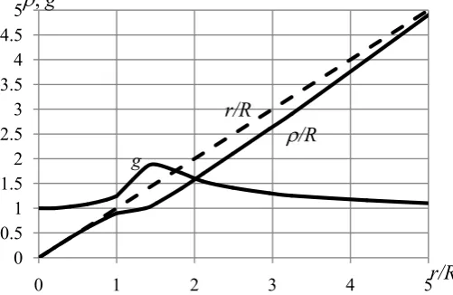
solu-tion becomes imaginary which means that the general relativity is not valid for such high levels of gravitation. Dependences of the space metric coefficients on the radial coordinate for the sphere with the critical radius Rg is shown in

Figure 1.

As can be seen, g r

(

→ ∞ =

)

1_and ρ → ∞ =

(

r

)

r_{(dashed line in}_Figure 1).

Consider the propagation of light from the sphere surface. The trajectory of light in the equatorial (θ = π 2_{) plane is specified by the following equations} [13]:

2

d ₁

d ee ee

h sh

r c

t q ρ

 

= _{− } _

  ,

2

d

d e_e

h cs t

ϕ ρ

  =  

  (40)

(9)

[image:9.595.247.498.76.239.2]

Figure 1. Dependences of the space metric coefficients on the radial coordinate for the

sphere with the critical radius.

2

d ₁

d

e e

r

e e

g r sh

v c

h t ρ

 

= = _{− } _

  ,

e e

sh

vϕ =c_ρ (41)

so that 2 2 2

r

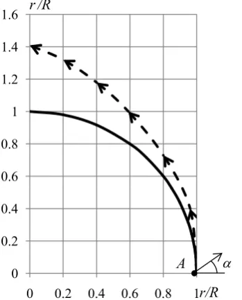
v +vϕ =c . Assume that light propagates from point A on the sphere

surface (ρ ρ= 1, r =1) at angle α with respect to the radius (Figure 2).

The initial conditions are vr=ccosα, vϕ =csinα and Equations (41) yield

1sin 1

s=ρ α h , where h h1= e

(

ρe =ρ1

)

. Consider the case α =0 for which

0

s= _and vr =c v, ϕ =0. This result allows us to conclude that in the radial di-rection light propagates for any spherical object with velocity c. However, if

0

α ≠ _{, the situation can be different. Using Equation (30) and Equation (40), we}

can obtain the following equation for the light trajectory:

2

2 2 2

1 1

d d d 1 ₁ 1 ₁

d d d sin

g g

e e

e

e e

r r

ρ ρ _ρ

ϕ ϕ ρ α ρ ρ ρ

   

= = _ − _− _ − _

    (42)

Numerical integration of this equation allows us to plot ρ ϕe

( )

. Using further Equation (38), we change ρe to r. The resulting trajectory r

( )

ϕ for α = π2 and r_g =0.5_{is shown in}_{Figure 2}_{with the dashed line. As follows from} Equa-tion (42), for the sphere with the critical radius, ρ1=rg the trajectory becomes

imaginary and light does not propagate.

Return to the internal problem and determine the stresses. Consider the first equation in Equation (28). Substitute qi from Equation (34) and express

(

)

(

2

)

2 1

i i r

i

i i

u h

h u

ρ ρ χσ

ρ ′ − ′

=

− (43)

Here, 2 ₃ 3

g

u=χµc =r R _{. Substitute Equation (43) in Equation (29) to get}

(

)

(

2

)

(

)

(

2

)

2 ₀

2 1

i i i

r r r r

i i

u c

u θ

ρ ρ ρ

σ σ σ χσ σ µ

ρ ρ

′ ′

′ − − + − − =

− (44)

The first equation for the stresses follows from this equation if we change variable r to ρ_{, use notations (19), and Equation (3), Equation (7) for} χ_and r_g, i.e.,

0 0.5 1 1.5 2 2.5 3 3.5 4 4.5 5

0 1 2 3 4 5

r/R

ρ

/R

ρ

,

g

(10)

[image:10.595.290.465.74.291.2]

Figure 2. Propagation of light from the sphere surface.

(

)

(

2

)

(

)(

)

d 2 _{1 3} ₁ ₀

d 2 1

g i r

r r r

i i g i

r r θ

ρ

σ _σ _σ _σ _σ

ρ +ρ − − − ρ − − = (45)

For a sphere of perfect fluid, σr =σθ = −p and Equation (45) reduces to

(

2

)

(

)(

)

d _{1 3} ₁ ₀

d 2 1

g i

i g i

r

p _p _p

r

ρ

ρ + − ρ + + =

The solution of this equation which satisfies the boundary condition p

(

ρi =ρ1

)

=0

is [10]

2 2

1

2 2

1

1 1

1 3 1

g i g

r r

p

r r

ρ ρ

− − −

=

− − − (46)

In contrast to the Schwarzchild solution, the pressure is not singular. For rg 1, Equation (46) degenerates into Equation (20). For the fluid sphere, Equation (43), being transformed to variables p, ,ρi rg, becomes

(

)

(

2

)

1 3 d

1

d 2 1

g i i

i i g i

r p

h

h r

ρ

ρ ρ

+ =

−

Integrating, we can find hi for the fluid sphere. The integration constant allows us to satisfy the last boundary condition in Equation (27).

To obtain the stresses, we need to supplement Equation (45) with an addi-tional equation. To derive this equation, we minimize the funcaddi-tional in Equation (15), where with regard to Equation (44)

(

)

(

)

(

)

(

) (

)

2 2 2

2 2

2 1 4

2

2 1

r r i i

i i r

i

r r r

i i

F q

u

c u

θ θ

θ

σ ν σ νσ σ ρ

ρ ρ χσ

ρ

λ σ σ σ σ µ

ρ ρ

 

=_ + − − _

 _′ _{′ −} 

 ′ 

+ + − + −

 − 

 

0 0.2 0.4 0.6 0.8 1 1.2 1.4 1.6

0 0.2 0.4 0.6 0.8 1

r /R

A

α

(11)

Using Equation (34) for qi, we can present the Euler equations, Equation (16), as

(

)

(

)

2 2

2

2 2 2 ( 2 0

2 1 1

i i i i

r r

i i

i

u c

u u

θ

ρ ρ ρ ρ

σ νσ λ χσ χµ λ

ρ ρ

ρ

 

′ ′_ _

′

− + + − + − =

 − 

− _ _

(

)

2

2 1 0

1

i r

i i

u θ

ρ λ

ν σ νσ

ρ ρ

− − − =

 

 

−

Expressing λ from the second equation, substituting in the first equation and reducing the resulting equation to the form similar to Equation (45), we arrive at

(

)

2 2

d ₂ ₂ 1 _{4 3} ₃ ₀

d 1

i r g i r

i g i

r r θ

σ

ρ σ νσ σ ρ σ

ρ ρ

 

 _ _

+ − + _ + _ − − __=

−

 

  (47)

where σ = −

(

1 ν σ

)

θ−νσr. For rg =0 and ρ =r, this equation coincides with

Equation (14). Numerical integration of Equation (45) and Equation (47) under the boundary conditions σ ρr

(

i =0

)

=σ ρθ

(

i =0

)

and σ ρr

(

i =ρ1

)

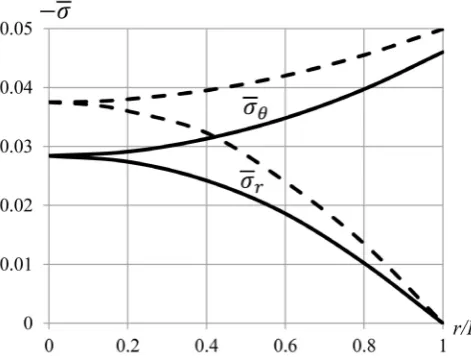
=0 allows

us to obtain the dependences of stresses on ρi which can be changed to r with the aid of Equation (38). The dependences σr

( )

r and σθ

( )

r corresponding

to rg =0.25 and ν =0 are shown in Figure 3 with solid lines. Dashed lines correspond to the linear classical solution in Equation (18).

3. The General Theory

Return to Section 1 and consider the general case. Ten Einstein’s equations

1 2

ij ij ij

R − g R=χT ₍₄₈₎

in which the energy tensor ij ij

T =σ

(

i j, =1,2,3

)

_, _Ti4₌₀

(

_i₌_1,2,3

)

_, _T44₌_µ_c2

[image:11.595.253.489.515.694.2]

satisfies the conservation equations

Figure 3. Dependences of the normalized stresses on the radial coordinate corresponding

(12)

2

44 0

ik i mk n ik i

kσ mkσ knσ µc

∂ + Γ + Γ + Γ = ₍₄₉₎

and includes 10 components of the metric tensor _gij_{. Because of Equation (49),} only six of Equation (48) are mutually independent and we have six equations for 16 functions, i.e., 10 coefficients _gij_{and six stresses} _σij_{. Assume that we} use six independent equations of Equation (48) to express six metric coefficients in terms of four. To derive four additional equations, we propose to use the vari-ational equation, Equation (31), in which six metric coefficients are expressed in terms of four. Variation with respect to these coefficients allows us to write four Euler’s equations and to obtain the set of 10 equations for the metric tensor.

To derive the equations for stresses, introduce the strain energy

1 2 3

1 _{d d d}

2 ij ij R

U =

_∫∫∫

σ ε g x x x

in which gR is the determinant of the metric tensor in the Riemannian three-dimensional space. Expressing strains in terms of stresses through Hooke’s la

ij mn cmnij

ε = σ

in which cmnij is the compliance tensor and introducing Equation (49) with aid

of the Lagrange multipliers, construct the augmented functional

1 2 3

1 _{d d d ,}

2

U=

_∫∫∫

F x x x

(

2

)

44

mn ij ik i mk n ik i

mnij R i k mk kn

F c= σ σ g +λ ∂ σ + Γ σ + Γ σ + Γ µc

Minimization with respect to the stresses and λ_{-multipliers yields 10 equations}

for six stresses and four multipliers [14]. Thus, we have arrived at the complete set of 20 equations for 10 metric coefficients 6 stresses and 4 multipliers.

4. Linearized Axisymmetric Problem

Spherically symmetric problem discussed above requires only one coordinate condition. To demonstrate a more complicated case, consider an axisymmetric problem for which we need two conditions. Since the general problem can hard-ly be solved because the equations are too complicated, obtain the linearized so-lution for the external space. The line element in cylindrical coordinates r, ,ϕ z

can be presented as

(

)

(

)

(

)

(

)

2 2 2 2 2 2 2

11 22 33 13 44

ds = +1 f dr +r 1+ f dϕ + +1 f dz + f r zd d − +1 f c td

Assume that functions fmn

( )

r z, are small in comparison with unity. For the

external space with zero stresses and density, Equations (1), i.e.

11 13 22 33 44 0

E =E =E =E =E = _{, reduce to}

(

)

(

)

(

)

(

)

2

13

22 44 33 44

2

22 44 11 22

2 0

0 f

r f f f f

r z

z

r f f f f

r z z

∂

∂ ∂

+ + + − =

∂ ∂

∂

∂ ∂

+ − − =

∂ ∂ ∂

(13)

(

)

(

)

(

)

(

)

2 2 2

13

33 44 11 44

2 2

2

22 44 11 22 44

2

2 0

f _f _f _f _f

r z r z

r f f f f f

r r

∂ ₋ ∂ ₊ ₋ ∂ ₊ ₌

∂ ∂ ∂ ∂

∂ ₊ ₋ ∂ ₋ ₋ ₌

∂ ∂

(51)

(

)

(

)

(

)

2

2 2

13

22 33 11 22

2 2

13

11 22 33

2

2 2 0

f

f f f f

r z

r z

f

f f f

r z

∂

∂ ₊ ₊ ∂ ₊ ₋

∂ ∂

− − − − =

∂ ∂

(52)

For the axially symmetric problem, we have two conservation equations, so only three of five Equations (50)-(52) are mutually independent. Consider Equation (52) and subtract from it the first equation in Equation (50) and the first equa-tion in Equaequa-tion (51). The resulting equaequa-tion

2 2

44 44 44

44 2 2

1 ₀

f f f

f

r r

r z

∂ ∂ ∂

∆ = + + =

∂

∂ ∂ (53)

allows us to conclude that f r z44

( )

, is the classical gravitational potential which

can be found in terms of exponential functions with respect to z and Bessel func-tions with respect to r [15]. For the external problem, the solution must satisfy the asymptotic conditions according to which f44→0 for r→ ∞ and

z→ ∞_{. Proceeding, express} f₁₃ from the first equation in Equations (50), i.e.,

(

)

2

(

)

13

33 44 2 22 44

1

2 2

f _f _f r _f _f

z r z

∂ ₌ ∂ ₊ ₊ ∂ ₊

∂ ∂ ∂ (54)

and substitute this result in the first equation in Equation (51) to get

(

)

(

)

3 2

22 44 11 22

2 2 0

r f f f f

r z z

∂ ₊ ₋ ∂ ₋ ₌

∂ ∂ ∂

This equation can be ignored because it follows from the second equation in Equation (50). Integration of Equation (50) yields

(

)

( )

11 22 22 44 1

f f r f f r

r ϕ

∂

= + − +

∂ (55) where ϕ1

( )

r is the integration function. Substituting Equation (55) in the

second equation of Equation (51), we get ϕ′ =1 0, so ϕ =1 C. Thus, Equation

(50) and Equation (51) allow us to express f13 and f11 in terms of two

un-known functions— f22 and f33. To proceed, we need to introduce two

coordi-nate conditions. As earlier, apply Equation (31), i.e., δ =D 0_{. The linearized}

space density is d= +1 f11+ f22+ f33. Using Equation (55), we can construct the

following functional:

d d d

D=

_∫∫∫

F r θ z, F r 1 2f22 r _r

(

f22 f44

)

f33 C ∂

 

= _ + + + + + _

∂

 

The condition δ =D 0 is satisfied if f33=0 and f22 is an arbitrary function.

To identify this function, we use, as earlier, the minimum condition d=1. Then, f22 = −f11 and Equation (55) yields

22 44

22

2

f f

r f r C

r r

∂ ∂

+ = −

(14)

The solution of this equation is

( )

22 11 2 44 2

1 _ln

f f f C r z

r ϕ

= − = _ − + _

Integration of Equation (54) allows us to find the last metric coefficient, i.e.,

( )

44 44

13 3 2 3

1 d

f f

f r z z r

z r r ϕ ϕ

∂ ∂ _′

= + + +

∂

∫

∂

Using the asymptotic conditions, we can conclude that constant C and functions

2, 3

ϕ ϕ are zero. Thus, the solution is

44

11 22 2

f

f f

r

= − = − , 44 44

13 f f d

f r z

z r

∂ ∂

= +

∂

∫

∂ , f33=0

where f44 is the solution of Equation (53). As follows from the foregoing

deri-vation, the space density is uniform in the external space.

5. Gravitation and Space Density

The space density introduced in Section 2.2 allows us to propose the new inter-pretation of gravitation. As follows from the foregoing discussion, the isolated object in space can be in equilibrium under the action of gravitation and stresses induced by gravitation. It is important that the gradient of the space density out-side the object is zero. Two objects in space cannot be in equilibrium and it is natural to suppose that the space density between them is not uniform. To take the equilibrium state and to reduce the gradient of the space density between the objects, they should move towards each other. Two situations are possible re-sulting in stable equilibrium or stable motion. First, the collision and the merge into one object can take place resulting in the equilibrium of the new object and zero gradient of the space density. Second case can take place if the trajectories of the moving objects are affected by perturbations induced by other objects in space. In this case, the collision does not occur and the objects orbit in elliptical paths.

6. Conclusion

The general relativity equations are supplemented with the coordinate condi-tions following from the stationarity condition of the three-dimensional metric tensor density and equations for the stresses similar to compatibility equations of the theory of elasticity. The solution of the obtained complete set of equations is demonstrated for linearized and general spherically symmetric problems and linearized axially symmetric problem. The space density which is the ratio of the three-dimensional metric tensor densities in Riemannian and Euclidean spaces in the same coordinates is introduced and used to explain the attraction of objects under the action of gravitation.

Conflicts of Interest

(15)

References

[1] Logunov, A.A., Mestvirishvili, M.A. and Petrov, V.A. (2004) Physics-Uspekhi, 47, 607-621.https://doi.org/10.1070/PU2004v047n06ABEH001817

[2] Landau, L.D. and Lifshits, E.M. (1988) Field Theory. Nauka, Moscow. (In Russian) [3] Arroyo-Torres, D., Wittkovski, M, Marcaide, J.M. and Hauschildt, P.H. (2013)

As-tronomy and Astrophysics, 554, A76.https://doi.org/10.1051/0004-6361/201220920

[4] Singe, J.L. (1960) Relativity: The General Theory. North-Holland Publishing Com-pany, Amsterdam.

[5] Schwarzschild, K. (1916) Sitz Preuss. Akad. Wiss., 189-207.

[6] Vasiliev, V.V. and Fedorov, L.V. (2018) Journal of Modern Physics, 9, 2482-2494.

https://doi.org/10.4236/jmp.2018.914160

[7] Schwarzschild, K. (1916) Sitz Preuss. Akad. Wiss., 424-432.

[8] Weinberg, S. (1972) Gravitation and Cosmology. John Wiley and Sons, Inc., New York.

[9] Fock, V. (1959) The Theory of Space, Time and Gravitation. Pergamon Press, Lon-don.

[10] Vasiliev, V.V. (2017) Journal of Modern Physics, 8, 1087-1100.

https://doi.org/10.4236/jmp.2017.87070

[11] Vasiliev, V.V. (1989) Mechanics of Solids, 5, 30-34.

[12] Schrodinger, E. (1950) Space-Time Structure. The University Press, Cambridge. [13] Logunov, A.A. (2006) Relativistic Theory of Gravitation. Nauka, Moscow. (In

Rus-sian)

[14] Vasiliev, V.V. and Fedorov, L.V. (2018) Mechanics of Solids, 53, 256-261.

https://doi.org/10.3103/S0025654418070038