doi:10.4236/iim.2012.23025 Published Online March 2010 (http://www.SciRP.org/journal/iim)
Adaptive Method for State Estimation of Sound
Environment System with Uncertainty and its Application
to Psychological Evaluation
Hisako Orimoto1, Akira Ikuta2
1Department of Circulation Information Engineering, Hiroshima National College of Maritime Technology, Hiroshima, Japan 2Department of Management Information Systems, Prefectural University of Hiroshima, Hiroshima, Japan
E-mail: [email protected], [email protected]
Received December 16, 2009; revised January 27, 2010; accepted February 28, 2010
Abstract
The actual sound environment system exhibits various types of linear and non-linear characteristics, and it often contains uncertainty. Furthermore, the observations in the sound environment are often in the level-quantized form. In this paper, two types of methods for estimating the specific signal for sound envi-ronment systems with uncertainty and the quantized observation are proposed by introducing newly a system model of the conditional probability type and moment statistics of fuzzy events. The effectiveness of the proposed theoretical methods is confirmed by applying them to the actual problem of psychological evalua-tion for the sound environment.
Keywords:Adaptive Estimation, Sound Environment System, Uncertainty, Psychological Evaluation
1. Introduction
The actual sound environment system contains uncer-tainty and it is often difficult to recognize analytically the internal physical mechanism. Furthermore, the stochastic process observed in the actual phenomenon exhibits complex fluctuation pattern and there are potentially various nonlinear correlations in addition to the linear correlation among the time series data.
In our previous study, a digital filter for estimating the state variables of complex stochastic systems was de-rived by introducing a nonlinear system model in an ex-pansion series of reflecting various type correlation in-formation from the lower order to the higher order be-tween state variable and observation [1]. The conditional probability density function in the expansion series con-tains the linear and nonlinear correlations in the expan-sion coefficients, and these correlations play an impor-tant role as the statistical information for the state vari-able and observation relationship.
On the other hand, it is necessary to pay our attention on the fact that the observation data in the sound envi-ronment system are often measured in a level-quantized form and contain fuzziness due to several causes. For example, the human psychological evaluation for loud-ness can be judged by use of 7 levels from 1.very calm to
7.very noisy [2]. However, each score is affected by the human subjectivity and the border between two neigh- boring scores are vague [3]. Furthermore, the observation data are often measured in a digital level form at discrete times because various kinds of statistical evaluation (e.g., median, mean, covariance, higher order moments, etc.) for these quantized level data become easier if a digital computer is used. Therefore, in order to evaluate the ob-jective sound environment system, it is desirable to esti-mate the waveform fluctuation of the specific signal for the system with uncertainty based on the quantized or fuzzy observation data.
esti-H. ORIMOTO ET AL. 213
mation algorithms are assumed accurate system and ob-servation models without containing uncertainty. On the other hand, the actual sound environment systems exhibit complex and unknown system characteristics and often contain uncertainty in the relationship among the state variables and the observation. Thus, it is necessary to improve the previous state estimation methods by taking account of the complexity and uncertainty in the actual systems.
In this paper, based on the quantized or fuzzy observa-tions, an adaptive method for estimating precisely the specific signal for the sound environment system with uncertainty is theoretically proposed. More specifically, first, by adopting an expansion expression of the condi-tional probability distribution reflecting the information on linear and nonlinear correlation among the time series of the specific signal and the quantized observation as the system and observation characteristics, a method to estimate adaptively the time series of the specific signal is derived. The proposed estimation method can be ap-plied to an actual complex sound environment system with uncertainty by considering the coefficients of con-ditional probability distribution as unknown parameters and estimating simultaneously these parameters and the specific signal. Next, by introducing fuzzy theory to the uncertainty of the system, the other type of estimation algorithm is derived. The proposed theory is applied to the estimation problem of the psychological evaluation for loudness in sound environment and the effectiveness of the theory is experimentally confirmed.
2. State Estimation of Sound Environment
System with Uncertainty
2.1. Estimation Algorithm by Introducing a Stochastic Model
Consider a complex sound environment system with un-certainty that cannot be obtained on the basis of the in-ternal physical mechanism of the system. In the observa-tions of actual sound environment system, the sound pressure level data are very often measured in a digital level form at discrete times. This is because some signal processing methods by utilizing a digital computer are indispensable for extracting exactly various quantities for human evaluation based on these quantized level data.
Let xk and be the input and output signals at a
discrete time for a sound environment system. For example, for the psychological evaluation in sound en-vironment,
k
y k
k
x and denote the physical sound pressure level and human response quantity for it, re-spectively. It is assumed that there are complex nonlinear relationships between
k
y
k
x and , which are difficult to find a fundamental relationship between them. Since
the system characteristics are unknown, a system model in the form of a conditional probability is adopted. More precisely, attention is focused on the joint probability distribution function reflecting all linear and nonlinear correlation information among
k
y
1
( ,k k , )k
P x x y
k
x , xk1
and . Expanding the joint probability distribution function in an orthogonal form based on the product of , and , the foll- owing expression can be derived.
k
y
1
( ,k k ,
P x x
(
P x
0 0 0
( ,k k
r s t
P x x
) k
y
)
k P x( k1)
(1) (1)
, ) ( ) (
( ) (
k k
rst r k s k
y P x P x
( )k
P y
(2)
) ( )
) (
k
t k
P y
1 1
1
k
)
A x x
) (1) ( 1
( )k s ( k ) t
A x x
y
( )yk
(1
rst r
(1)
with
2)
(2)
where < > denotes the averaging operation on the vari-ables. The linear and nonlinear correlation information among xk, xk1 and is reflected hierarchically in
each expansion coefficient
k
y
rst
A . The functions (1)( )
r xk
P x
(
s x
) k
and are orthonormal polynomials with the weighting functions and , respectively. These orthonormal polynomials can be decomposed by using Schmidt's orthogonalization [12]. From (1), the conditional probability distribution function
and are given as
(2)
P y
P x
P y ( )
t yk
( k|xk)
( k |xk)P
( k|xk)P
0
rs
( )k P x
1 1
0 0
( k ) R S rs
r s
x A
(1) 0 0 0
( )k R T r t r r t
y A
( )k
(1) 0r ( )xk
(2)
) (
k t y
P y
1
( k |xk
1)
)
(1)
k (3)
(x (4) Though (3) and (4) are originally infinite series expan-sions, finite expansion series are adopted because only finite expansion coefficients are available and the con-sideration of the expansion coefficients from the first few terms is usually sufficient in practice. Since the objective system contains an unknown structure, the expansion coefficients A and Ar t0 expressing hierarchically
the correlation relationship between xk, xk1 and xk, have to be estimated on the basis of the observation . Considering the expansion coefficients
k
y
k
y Ars0 and
0
r t
A as unknown parameter vectors a and : b
( )
, )
, 2, ...,
I S
1 2 1 0 2 0
, , ...,
( ,
s s
a a (1) (2)
0
) ( , ,
, ..., ), (
s Rs
a
( )
( ...
1 )
A A A
a a
(1) (2)
) ( , ,
..., ), ( 1
b
s S
a a
( ))
2, ...,
J T
a
(
(5)
1, 2, ...,
( , ,
b b
( ) 10 20 0
..., ,
t A t A t AR t )
b b
t T
b b
)
where I ( R S and J ( R T) are the number of unknown expansion coefficients to be estimated, the simple dynamical models:
1 , 1
k k k
a a b bk (7) are introduced for the simultaneous estimation of the parameters with the specific signal xk.
To derive an estimation algorithm for the specific sig-nal xk, attention is focused on Bayes' theorem for the conditional probability distribution [12,13]. Since the parameter and are also unknown, the condi-tional probability distribution of
k
a bk
k
x , and is considered.
k
a bk
1 1
( , , , | ( , , | )
( | )
k k k k k
k k k k
k k
P x y Y
P x Y
P y Y
a b
a b ) (8)
where is a set of observation data up to time . The conditional joint probability distribu-tion 1 can be generally expanded in a statistical orthogonal expansion series:
1 2
( { , ,..., }) k
Y y y y k
( , ,k k k, k| k )
P x a b y Y
k
y
1
0 1 0 1 0 1 0 1 (1) (2) (3) (4) 0 0
( , , , | )
( | ) ( | ) ( | ) ( | )
( ) ( ) ( ) ( )
k k k k k
k k k k k k k k
l q l k k k q k
l q
P x y Y
P x Y P Y P Y P y Y
B x
mn m nm 0 n 0
a b
a b
a b (9)
(1) (2) (3) (4)
1
( ) ( ) ( ) ( ) |
l q l k k k q k k
Bmn x m a n b y Y (10) After substituting (9) into (8) and expanding an arbitrary polynomial function fL, ,M N( , ,xk a bk k) of xk, and
with th order in a series expansion form using
k
a
k
b ( , , )LM N
(1)
{l ( )}xk , { (2)( )} and { ( :
k
m a
(3)
n
bk)}
(1) (2) (3) , ,
0
( , , ) L L ( ) ( ) ( )
L k k k l l k k k
l
f x C x
M N MNM N mn m n
m 0 n 0
a b a b
( L ; appropriate constants), (11)
l
C MN mn
by taking the conditional expectation of the function
, , ( , , )
L k k k
f M N x a b and using the orthonormal condition for the functions (1)( )
l xk
, and , the
estimate of the function
(2)( )
k
m a
, , ( ,
(3)( )
k
n b
) ,
L k k
f M N x a bk can be
de-rived as follows:
, , , , (4) 0 0 (4) 0 0
ˆ ( , , ) ( , , ) |
( )
( )
L k k k L k k k k
L
L
l l q q k
l q
q q k
q
f x f x Y
C B y
B y
M N M N
M N
MN
mn mn
m 0 n 0
00
a b a b
(12)
The four functions , , and
are orthonormal polynomials of degrees l,
, and with weighting functions ,
, and , which can
be chosen as the probability functions describing the dominant parts of the actual fluctuation or as the well-known standard probability distributions.
) ( ) 1 ( k l x
m(2)(ak) n(3)(bk)
) ( ) 4 ( k q y m n ( | q ) P x
0( k| k1)
P x Y
1) 0 k k1
P a Y P0(bk|Yk)
0( k|Yk1) N
1 P y Y0( k| k
*
; ,xk xk)
As an example of standard probability functions for the specific signal and the parameter, consider the Gaus-sian distribution:
(xk
,
* , ,
( i k; i k, a N a a
,
* , ,
( i k; i k, b N b b
(13)
0( | 1)
I
k k
i
P Y
0( k| k 1)
i
P Y
1 ) i k ) i k a b (14) 1 J
(15) with , , 2 2 2 * * * * 1 , * *1 , ,
( )
1 exp{ }
2 2 | , ( ) | | , ( | , ( k i k i k k
k x k k
k a i k i k
k b i k i k
x
Y x x
Y a a
Y b b
2 , , , , ) i k i k 2 1 1 , 1 1 , , ) | , ) | . k k k Y Y Y 2 2 ( ; , k k x x a a b b i k i k N x y h , )
k hy
(16) Furthermore, as the fundamental probability function on the level-quantized observation, the generalized binomial distribution [14] with level difference interval can be chosen:
0( k|Yk1) B y N( ;k yk,M py, y
P y (17)
with * * ( ; , , k y k N M
y M *
1
* *
* 2 1
( )!
) (1 ) ,
( )!( )! , | , , ( ) | , k k
y M N y
h h
y k k k
y k y y
k y y y
k k
N M
h p p
y M N y
h h
p y y Y
h y M h Y , ( ) ( ) k y y y k y p h N M y M y M y y k k k y B y N y (18)
where M is the minimum level of the observation. The orthonormal polynomials with four weighting prob-ability distributions in (13)-(15) and (17) can be deter-mined as
* (1)( ) 1 ( )
! k
k k
l k l
x x x x H l
(19)
, * , , 1 1 ( ) ( ) ! i i k I
i k i k
k m
i i a
a a H m
a (2)H. ORIMOTO ET AL. 215
,
* , , (3)
1
1
( ) ( )
! i i k
J
i k i k
k n
i i b
b b
H n
n b (21)
(4)( ) ( ; , , , )
k k
q yk BP y Nq k y M p hy y y
(22)
with
( ) 1/ 2 / 2
( ) ( ) 0
1
( ; , , , ) {( ) !} ( )
1
( 1) ( ) ( ) ( )
1
q q
q
q
q j q j q j j
q j
N M p
BP y N M p h q
h p
q p
N y y M
j p
h
(23)where denotes the Hermite polynomial with th order [15], and
( ) l
H l
( )j
y is the th order factorial function defined by [14]
j
( )n ( )( 2 ) ( ( 1) ), (0)
y y y
y y y h y h y n h y 1 (24) Using the property of conditional expectation and (3)(4), the two variables * and
k
y yk in (18) can be ex-pressed in functional forms on predictions of xk,
and at a discrete time
k
a
k
b k1 (i.e., the expectation value of arbitrary functions of xk, and
condi-tioned by ), as follows:
k
a bk
1
k
Y
*
1 1
(1)
1 0 1
0 0 1
(1)
1 0 1 1
0 0 1
1 0 ( ), 1 1 0 0
( | ) |
( ) |
( ) ( | ) |
( ) | ,
k k k k k k
t r t r k k
r t
t r t r k k k k k
r t
t r t r k k k
r t
y y P y x dy Y
d A x Y
d A x P x x dx Y
d A x Y
A (25)* 2
1 2
2 0 ( ), 1 1 0 0
( ) ( | ) |
( ) |
k k k k k k k
t r t r k k k
r t
y y P y x dy Y
d A x Y
A k
)
2 2
0 k
(26)
with
( ), ( ), (0),
(1) (1) (1) 0 1
(0, ), ( 1, 2, ), (1, 0, 0, , 0),
( ) ( ( ), ( ), , ( )) ',
r k r k
k
k k k R
r
x x x x
A a
A
(27) where ' denotes the transpose of a matrix. The coeffi-cients and in (25) and (26) are determined in advance by expanding and in the fol-lowing orthogonal series forms:
1t
d d2t k
y ( * 2
k k
y y
1
(2) * 2 (2) 1
0
( ), ( ) ( )
k i i k k k i i
i i
y d y y y d y
(28)Furthermore, using (3) and (4), and the orthonormal con-dition of (1)( )
i xk
and , each expansion
coeffi-cient defined by (10) can be obtained through the similar calculation process to (25) and (26), as follows:
(2)( )
i yk
l q
Bmn
l q
(2) (3) ,
0 0 0
0 ( ), 1 1
( )
( ) ( ) |
q l r
qt l r j k
r t j
k r t j k k k
B d w
A x Y
m a nb A
mn
qi
d
(4)
(1)
(29)
where and are appropriate coefficients sat-isfying the following equalities:
,
l r j
w
(2) 0
(1) (1) , 0
( ) ( ),
( ) ( ) ( )
q
q k qi i k
i
l r
l k r k l r j j k
j
y d y
x x w x
(30)Furthermore, by substituting the dynamical models of and in (7) into (25), (26) and (29), the parame-ters and
k
a bk
*
k
y yk and the expansion coefficient can be given in functional forms on estimations of
l q
Bmn
1
k
x ,
1
k
a and bk1. Therefore, the recurrence estimation of the specific signal can be achieved.
2.2. Estimation Algorithm by Introducing a Fuzzy Theory
In the observations of actual sound environment system, the sound pressure level data often contain fuzziness due to human subjectivity in noise evaluation, confidence limitations in sensing devices, and quantizing errors in digital observations, etc. Let be fuzzy observation obtained from . For example, for the psychological evaluation in sound environment,
k
z
k
y
k
x and denote respectively the physical sound pressure level and human response quantity for it. Since the system characteristics are unknown, the observation model in a form of a con-ditional probability in (4) is adopted. Furthermore, expresses the loudness scores (1.very calm, 2.calm, 3.mostly calm, 4.little noisy, 5.noisy, 6.faily noisy, 7.very noisy) taking the individual and psychological situation into consideration for . The fuzziness of is characterized by the membership function
k
y
k
z
k
z
( ) k
y
k
z yk
.
As the membership function, a standard Gaussian type function:
2
( ) exp{ ( ) }
k
z yk yk k
z , (31) where ( 0) is a parameter, is adopted. Though the parameter in (31) can be generally given based on the prior information (or, through trial and error), it can be regarded as unknown parameter and estimated simul-taneously with the specific signal xk and the parameter
. First, a simple dynamical model for the parameter:
k
k
1
k
, (32) is naturally introduced. Next, as the similar manner to (8), by paying our attention to the conditional joint probabil-ity densprobabil-ity function of xk, bk and k, the following expression is obtained.
1 1 0 1 0 1 0 1
(1) (3) (5) (6) 0 0 0
(6) 0 0 0 ( , , , | ( , , | ) ( | ) ( | ) ( | ) ( | ) ( ) ( ) ( ) ( ) ( )
k k k k k
k k k k
k k
k k k k k k
l nq l k k n k q k
l n q
q q k
q
P x z Z
P x Z
P z Z
P x Z P Z P Z
D x D z z
m m m 0 0 b b b b ) (33) with(1) (3) (5) (6)
1
( ) ( ) ( ) ( ) | ,
l nq l k k n k q k k
Dm x m b z Z (34) where Zk( { , ,..., }) z z1 2 zk is a set of fuzzy observation
data. The two functions (5)( )
n k
and denote
the orthonormal polynomials of degrees and , with the fundamental probability density functions
(6)( )
q zk
n q
0( |
P k Zk1) and P z0( |k Zk1) of k and as weighting functions. Based on (33), through the similar calculation process to (12), the estimate of an arbitrary polynomial function
k
z
, , ( , , )
L N k
f M x bk k of xk, bk and k
of ( , , )L M N th order can be derived, as follows:
, , , ,
(6) 0 0 0
(6) 0 0 0
ˆ ( , , ) ( , ) |
( )
( )
L N k k k L N k k k k
L N
L N
l n l nq q k
l n q
q q k
q
f x f x Z
E D z
D z
M M M M m m m 0 0 b b (35)All the coefficients L N l n
E M
m are appropriate constants in
the case when the function fL, ,MN( ,xk bk,k) is ex-pressed in a series expansion form similar to (11) using
(1)
{l ( )}xk , and . As concrete ex-amples of the fundamental probability density functions for the parameter
(3)
{m (bk)}
k
(5)
{ n ( )}k
and , the Gaussian distribution and the generalized binomial distribution are adopted, respectively:
k
z
* 0( k | k 1) ( ;k k, k)
P Z N (36)
0( |k k 1) ( ;k zk, z, zk, )z
P z Z B z N M p h (37) with * * 1 1 * * 1 | , ( ) | , , | , k k k
k k k k k k
k z
z k k k
z z
Z Z
z M
p z z Z
N M * * * ( ) , ( ) k k k
k z z k z z
z
k z z z
z M h z M N
z M h
* 2 1 ( ) | k
z zk zk Zk ,
(38) where Mz is the minimum level of the observation
and
k
z
z
h denotes the level difference interval of . Then, the orthonormal polynomials with two weighting probability density functions in (36) and (37) can be given as
k
z
* (5)( ) 1 ( )
! k
k k
n k Hn
n
, (39)
(6)( ) ( ; , , , )
k k
q zk BP z Nq k z M p hz z z
. (40)
After applying moment statistics of fuzzy events which are generalization of mean and variance of fuzzy events [16], by applying (4), the two variables * and
k
z zk in (38) and the expansion coefficient are expressed in concrete forms, as follows:
l nq Dm 1 * 1 ( ) | , ( ) | k k
z k k k
k
z k k
y y Z z y Z
(41)
* 2 1 1 ( )( ) | , ( ) | k k k
z k k k k
z
z k k
y y z Z
y Z (42)
(1) (3) (5) (6)
1 1 ( ) ( ) ( ) ( ) ( ) | ( ) | . k k
l nq l k k n k z k q k k
z k k
D x y y Z
y Z
m m b
(43) Furthermore, by applying (4) and considering orthonor-mal condition of , (41)–(43) can be expressed as follows:
(2)( )
t yk
( ), 1 * 0
( ), 1 0
( ) |
( ) | T
t t k k k
t
k T
t t k k k
t
e x Z
z
h x Z
B B (44)( ), 1 0
( ), 1 0
( ) |
( ) |
k
T
t t k k k
t
z T
t t k k k
t
f x Z
h x Z
B B (45)(1) (3) (5)
( ), 1 0
( ), 1 0
( ) ( ) ( ) ( ) |
( ) | T
l nq t l k k n k t k k k
t T
t t k k k
t
D g x x Z
h x Z
m m b B
B
(46)
2
with
( ),t k(0, ( ),t k), (t1, 2, ), (0),k (1, 0, 0, , 0),
B b B
H. ORIMOTO ET AL. 217
where et, ft, gt and are expansion coefficients
satisfying the following relations:
t
h
(2) 0
( ) ( )
k
z k k i i k
i
y y e y
(48)* 2 (2) 0
( )( ) ( )
k
z k k k i i k
i
y y z f y
(49)(6) (2) 0
( ) ( ) ( )
k
z k r k i i k
i
y y g y
(50)(2) 0
( ) ( )
k
z k i i
i
y h y
k (51)The variables * ,
k
z zk and expansion coefficient
in (44)–(46) can be given by the predictions of
l nq
Dm
k
x , and . Furthermore, the following simple system model is introduced instead of (3), for the simpli-fication of the algorithm.
k
b k
1
k k k
x Fx Gu (52) where is the random input with mean 0 and variance
, and
k
u
2
u
F, are system parameters. By considering (7) (32) and (52), the prediction algorithm for an
arbi-trary polynomial function with
th order can be given as follows: G
, , ( 1, 1, 1
L N k k k
g M x b )
( , , )L M N
*
, , 1 1 1 , , 1 1 1 , ,
( , , ) ( , , ) |
( , , ) |
L N k k k L N k k k k
L N k k k k k
g x g x Z
g Fx Gu Z
M M
M
b b
b
(53) Since the prediction of xk1, and at a
dis-crete time in (53) are given in the form of estimates for the polynomial functions of
1
k
b k1
k
k
x , bk and k, by
combining the estimation algorithm of (35) with the pre-diction algorithm of (53), the recurrence estimation of the specific signal can be obtained.
3. Application to Psychological Evaluation
for Loudness
To find the quantitative relationship between the loud-ness for human and the physical sound pressure level for environmental noise is important from the viewpoint of noise assessment. Especially, in the evaluation for a re-gional sound environment, the investigation based on questionnaires to the regional inhabitants is often given when the experimental measurement at every instanta-neous time and at every point in the whole area of the region is difficult. Therefore, it is very important to esti-mate the sound pressure level based on the loudness data. It has been reported that the loudness based on the hu-man sensitivity can be distinguished each other from 7
loudness scores, for instance, 1.very calm, 2.calm, 3.mostly calm, 4.little noisy, 5.noisy, 6.fairly noisy, 7.very noisy, in the psychological acoustics [2]. After recording the road traffic noise by use of a sound pres-sure level meter and a data recorder, by replaying the recorded tape through amplifier and loudspeaker in a laboratory room, 6 subjects (A, B, …, F) aged of 22-24 with normal hearing ability judged one score among 7 loudness scores (i.e., 1, 2, …, 7) at every 5 [sec.], ac-cording to their impressions for the loudness at each moment using 7 categories from very calm to very noisy. The mean and standard deviation of the road traffic noise were 71.4 [dB] and 7.23 [dB], respectively. Furthermore, the mean and standard deviation for the loudness scores of each subject, and the correlation coefficients between the road traffic noise levels and the loudness scores are shown in Table 1.
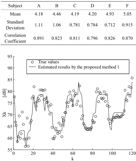
The state estimation method proposed in Subsection 2.1 was applied to an estimation of the time series xk for sound pressure level of a road traffic noise based on the successive judgments on loudness scores. Figure 1 shows one of the estimated results of the waveform fluc-tuation of the sound pressure level based on the loudness score by a subject. In this figure, the horizontal axis shows the discrete time , of the estimation process,
k
y
[image:6.595.307.538.421.695.2]k
Table 1. Statistics of loudness scores and correlation coeffi-cients between the sound pressure level and the loudness scores.
Subject A B C D E F Mean 4.18 4.46 4.19 4.20 4.93 5.05 Standard
Deviation 1.11 1.06 0.781 0.784 0.712 0.915 Correlation
Coefficient 0.891 0.823 0.811 0.796 0.826 0.870
0 20 40 60 80 100 120
55 60 65 70 75 80 85 90 95
k
Xk
[
dB]
True values
Estimated results by the proposed method 1
)
and the vertical axis represents the A-weighted sound pressure level (i.e., the sound pressure level measured by use of sound level meter with frequency weight of A-type characteristic). The finite numbers of expansion coefficients in the proposed estimation algorithm (12) employing the system models of condi-tional probability type (3) and (4) with
were used in this estimation. In principle, it is expected that the successive addition of higher expansion terms reflecting higher order statistics in the proposed algo-rithm moves the theoretical estimation closer to the true values. However, higher order statistics based on the finite numbers of observed sample data give us unstable information with less reliability. It remains as one of the future problems to derive a method for determining an optimal order for the conditional probability distribution in expansion series form like (3) and (4).
l q
Bmn (q2
2
R S T
One of the estimated results by applying the algorithm proposed in Subsection 2.2 is shown in Figure 2. Fur-thermore, the estimated processe for the parameter of the membership function in (31) is shown in Figure 3. The estimated parameter converges to a certain value as considering sequentially the observation data. The esti-mated results of the parameter of the membership function in (31) are shown in Table 2 for all subjects.
For comparison, the estimated results by the previ-ously reported method [1] and the extended Kalman Fil-ter [6] are shown in Figure 4. The root mean squared error of the estimation is shown in Table 3. It is obvious that the proposed methods show more accurate estima-tions than the results based on the previous estimation method and the extended Kalman filter. By comparing Table 3 with Table 1, it can be found that the more ac-curate estimation results are obtained in cases with the larger values of the correlation coefficient between the sound pressure levels and the loudness scores.
0 20 40 60 80 100 120
55 60 65 70 75 80 85 90 95
k
Xk
[
dB
]
True values
Estimated results by the propsed method 2
Figure 2. Estimation results of the sound pressure level by use of the method in Subsection 2.2.
0 20 40 60 80 100 120
0.04 0.06 0.08 0.1 0.12 0.14 0.16 0.18
k
Estimated result of the parameter of membership function
Figure 3. One of the estimation results for the parameter of the membership function.
0 20 40 60 80 100 120
50 55 60 65 70 75 80 85 90 95 100
k
Xk
[
dB
]
True values Estimated results by the previous method Estimated results by the extended Kalman filter
Figure 4. Estimation results of the sound pressure level by use of the previous method and the extended Kalman filter.
Table 2. Estimated results of the parameter of the mem-bership function in (31).
Subject A B C D E F
Estimates 0.161 0.201 0.483 0.231 0.241 0.245
Table 3. Root means squared error of the estimation in [dB].
Sublect A B C D E F
Method 1 in
Section 2.1 3.13 3.67 3.88 3.97 3.61 3.16 Method 2 in
Section 2.2 3.15 3.93 4.32 4.13 3.82 3.44 Previous
Method 3.94 4.89 4.56 4.28 3.91 3.59 Extended
H. ORIMOTO ET AL. 219
4. Conclusions
In this paper, based on the quantized or fuzzy observa-tion data, two types of new methods for estimating the specific signal for sound environment systems with un-certainty have been propoesd. The proposed estimation methods have been realized by introducing a system model of conditional probability type and a fuzzy theory. The proposed methods have been applied to the estima-tion of an actual sound environment, and it has been ex-perimentally verified that better results have been ob-tained as compared with the results by use of the previ-ous method and the extended Kalman filter.
The proposed approach is quite different from the tra-ditional standard approaches. It is still at early stage of development, and a number of practical problems are yet to be investigated in the future. These include: 1) Appli-cation of the proposed state estimation methods to a di-verse range of practical estimation problems for stochas-tic systems with uncertainty. For example, the proposed methods have to be applied to the observation data for human psychological evaluation in many fields in order to estimate the physical quantities. 2) Extension of the proposed methods to cases with multi-dimensional state variable and multi-source configuration. 3) Finding an optimal number of expansion terms in the proposed es-timation algorithm of expansion expression type. 4) Ex-tension of the proposed theory to the actual situation un-der existence of the external noise (i.e., background noise).
5. Acknowledgement
The authors are grateful to Prof. M. Ohta for his helpful discussion during this study.
6. References
[1] A. Ikuta, H. Masuike, and M. Ohta, “A digital filter for stochastic systems with unknown structure and its appli-cation to psychological evaluation of sound environ-ment,” IEICE Transactions on Information and Systems, Vol. E88-D, No. 7, pp. 1519–1522, 2005.
[2] S. Namba, S. Kuwano, and T. Nakamura, “Rating of road traffic noise using the method of continuous judgment by category,” The Journal of the Acoustical Society of Japan, Vol. 34, No. 1, pp. 29–34, 1978.
[3] A. Ikuta, M. Ohta, and M. N. H. Siddique, “Prediction of probability distribution for the psychological evaluation of noise in the environment based on fuzzy theory,” In-ternational Journal of Acousics and Vibration, Vol. 10, No. 3, pp. 107–114, 2005.
[4] R. E. Kalman, “A new approach to linear filtering and
prediction problems,” Transactions of ASME, Series D, Journal of Basic Engineering, Vol. 82, No. 1, pp. 35–45, 1960.
[5] R. E. Kalman and R. S. Bucy, “New results in linear fil-tering and prediction theory,” Transactions of ASME, Se-ries D, Journal of Basic Engineering, Vol. 83, No. 1, pp. 95–108, 1961.
[6] H. J. Kushner, “Approximations to optimal nonlinear
filter,” IEEE Transactions on Automatic Control, Vol. 12, No. 5, pp. 546–556, 1967.
[7] B. Bell and F. W. Cathey, “The iterated Kalman filter
update as a Gauss-Newton methods,” IEEE Transactions on Automatic Control, Vol. 38, No. 2, pp. 294–297, 1993. [8] K. Nishiyama, “A nonlinear filter for estimating a
sinu-soidal signal and its parameter: On the case of a signal sinusoid,” IEEE Transactions on Signal Processing, Vol. 45, No. 5, pp. 970–981, 1997.
[9] T. L. Vincent and P. P. Khargonekar, “A class of nonlin-ear filtering problems arising from drift sensor gains,” IEEE Transactions on Automatic Control, Vo. 44, No. 3, pp. 509–520, 1999.
[10] S. Julier and J. Uhlmann, “Unscented filtering and
nonlinear estimation,” Proceedings of The IEEE, Vol. 92, No. 3, pp. 401–421, 2004.
[11] G. Kitagawa, “Monte carlo filter and smoother for
non-Gaussian nonlinear state space models,” Journal of Computational and Graphical Statistics, Vol. 5, No. 1, pp. 1–25, 1996.
[12] M. Ohta and H. Yamada, “New methodological trials of
dynamical state estimation for the noise and vibration en-vironmental system,” Acustica, Vol. 55, No. 4, pp. 199– 212, 1984.
[13] A. Ikuta and M. Ohta, “A state estimation method of
impulsive signal using digital filter under the existence of external noise and its application to room acoustics,” IEICE Transactions on Fundamentals of Electronics, Communications and Computer Sciences, Vol. E75-A, No. 8, pp. 988–995, 1992.
[14] M. Ohta and A. Ikuta, “A basic theory of statistical gen-eralization and its experiment on the multi-variate state for environmental noise---A unification on the variate of probability function characteristics and digital or ana-logue type level observation,” The Journal of the Acous-tical Society of Japan, Vol. 39, No. 9, pp. 592–603, 1983. [15] M. Ohta and T. Koizumi, “General statistical treatment of
the response of a non-linear rectifying device to a sta-tionary random input,” IEEE Transactions on Information Theory, Vol. 14, No. 4, pp. 595–598, 1968.
[16] L. A. Zadeh, “Probability measures of fuzzy events,”