Simultaneous localization and mapping in wireless sensor networks

http://wrap.warwick.ac.uk/

Original citation:

Dumont, Thierry and Le Corff, Sylvain. (2014) Simultaneous localization and mapping in

wireless sensor networks. Signal Processing: Image Communication, Volume 101

(Number 2). pp. 192-203.

Permanent WRAP url:

http://wrap.warwick.ac.uk/59645

Copyright and reuse:

The Warwick Research Archive Portal (WRAP) makes this work of researchers of the

University of Warwick available open access under the following conditions.

This article is made available under the Creative Commons Attribution- 3.0 Unported

(CC BY 3.0) license and may be reused according to the conditions of the license. For

more details see

http://creativecommons.org/licenses/by/3.0/

A note on versions:

The version presented in WRAP is the published version, or, version of record, and may

be cited as it appears here.

Simultaneous localization and mapping in wireless

sensor networks

Thierry Dumont

, Sylvain Le Corff

a

Laboratoire MODAL'X, Université Paris Ouest Nantere La Défense, France b

Department of Statistics, University of Warwick, United Kingdom

a r t i c l e i n f o

Article history:

Received 28 February 2013 Received in revised form 24 January 2014 Accepted 14 February 2014 Available online 22 February 2014

Keywords:

Simultaneous localization and mapping Indoor localization

Received signal strength indicator Parameter estimation

Signal propagation

a b s t r a c t

Mobile device localization in wireless sensor networks is a challenging task. It has already been addressed when the WiFi propagation maps of the access points are modeled deterministically or estimated using an offline human training calibration. However, these techniques do not take into account the environmental dynamics. In this paper, the maps are assumed to be made of an average indoor propagation model combined with a perturbation field which represents the influence of the environment. This perturbation field is embedded with a distribution describing the prior knowledge about the environ-mental influence. The device is localized with Sequential Monte Carlo methods and relies on the estimation of the propagation maps. This inference task is performed online, using the observations sequentially, with a new online Expectation Maximization based algorithm. The performance of the algorithm is illustrated with Monte Carlo experiments using both simulated data and a true data set.

&2014 The Authors. Published by Elsevier B.V. This is an open access article under the CC

BY license (http://creativecommons.org/licenses/by/3.0/).

1. Introduction

In this paper, we consider a WiFi communication net-work made up of a mobile device, a server and WiFi access points (AP). In this context, a key step to localize the mobile device is to estimate the WiFi signal strength at different positions in the environment. However, in an indoor environment, signals may experience complex attenuation such as shadowing or reflection.

Different techniques can be used to approximate the WiFi propagation map of each AP. In Gorce et al. [19], a deterministic model based on the characteristics of the sur-rounding AP and on the localization of the obstacles in the

environment is introduced. In Bahl and Padmanabhan[2] and Evennou and Marx [16], a previous offline training phase is performed. In this site survey, the signal strength indicator (RSSI) received from different AP is measured at some previously determined positions. This allows us to build an accurate estimation of the signal strength, but only for a finite number of points. Ferris et al. [17] provide a method to extend these measures to the entire map using Gaussian processes techniques.

In this paper, we propose an estimation method that does not require any calibration procedure. The propagation maps are estimated online, without storing the observations, using the data sent by the mobile device. Any modification in the signal propagation (due to new obstacles for instance) affects the data sent by the mobile device. Then, while these changes deteriorate the accuracy of localization systems based on fixed estimators of the propagation maps, our estimation procedure takes them into account. Thus, as illustrated in Section 5.2, the accuracy of our localization method improves with time instead of degrading.

Contents lists available atScienceDirect

journal homepage:www.elsevier.com/locate/sigpro

Signal Processing

http://dx.doi.org/10.1016/j.sigpro.2014.02.011

0165-1684&2014 The Authors. Published by Elsevier B.V. This is an open access article under the CC BY license

(http://creativecommons.org/licenses/by/3.0/).

n_{Corresponding author.}

E-mail addresses:[email protected](T. Dumont),

[email protected](S. Le Corff).

1_{This work is partially supported by ID Services, 91400 Orsay, France.} 2

We use a semiparametric statistical model introduced in [15, Chapter 5]: the propagation maps are made of a parametric average indoor model and a nonparametric perturbation field. This model combines a prior knowledge on signal propagation with random perturbations due to the obstacles. Based on the data collected by the mobile device, the parameters and the perturbation field can be estimated. The proposed procedure relies on a new online Expectation Maximization (EM) based algorithm intro-duced in Le Corff and Fort [21,22] and on Sequential Monte Carlo methods. The device position can be simulta-neously estimated using the weighted samples produced by the Sequential Monte Carlo method.

The structure of this paper is the following. Section 2 details the approach of the paper in comparison with other methods for localization and mapping in wireless sensor networks.Section 3 describes the model and defines the notations. Section 4 introduces our algorithm for the considered Simultaneous Localization and Mapping (SLAM) problem.Section 5illustrates the performance of this algorithm with numerical experiments.

2. State of the art and main contributions

2.1. Wireless sensor networks

In a radio network field, the signal strength is measured by the RSS (received signal strength, in dBm). Each WiFi connected device can compute the RSS as it is needed to associate the device with the AP providing the best signal/ noise ratio. Localization systems based on RSS measure-ments allow us to locate any WiFi connected device.

Remark 1. Different devices might have different methods to

compute the RSS. It is common to use the terminology of RSSI (received signal strength indicator) expressed without unit to name the information on the signal level provided by a WiFi device. To overcome the issue of information disparity between WiFi connected devices, a previous RSSI to RSS conversion might be needed for each localized device. The conversion rule is specific to the device's WiFi card. For the sake of clarity, we assume in this paper that the mobile device's RSSI corresponds to the standard RSS.

Using RSS to estimate the position of the device is challenging. As represented inFig. 1, RSS is highly unstable as it fluctuates considerably between two consecutive measures at the same position. It is common to describe the RSS variations using a Gaussian representation.

Despite the instant variations of the RSS, its mean value strongly depends on the position of the device. The function that returns the expected RSS at each position is called thepropagation map. In free spaces, signals propa-gate in straight line from the emitter to the receptor. The propagation maps are isotropic and can be described using few parameters, see Friis [18]. Therefore, there exist two parameters c and d such that the strength of a signal received atxand emitted atOiscþdlogðJxOJÞwherec

andddepend on the network characteristics.

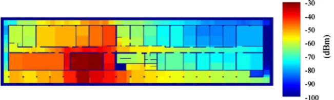
On the other hand, indoor propagation of WiFi signals is not isotropic.Fig. 2represents thepropagation mapof a WiFi signal in an indoor environment. This figure was built deterministically by Gorce et al. [19] using the physical properties of electromagnetic signals.

2.1.1. General model for signal propagation

LetXkbe the device position at time k. The received

signal strength vector measured by the device, denoted by

Yk, is written as

Yk¼F⋆kðXkÞþϵk: ð1Þ

In the following, the superscript⋆is used to name the true value of every unknown parameter involved in the model.

fϵkgkZ0 are i.i.d. multidimensional random variables with distributionNð0;s⋆;2_{IdÞwhereIdis the identity matrix. Each} component ofF⋆_kðxÞrepresents the expected RSS at positionx

relative to an AP. The time dependency of F⋆ brings the environmental effects on the propagation maps into relief. The distribution offϵkgkZ0implies that the noise affecting the RSS of different AP are independent. This assumption is somehow strong, however, the correlation between the RSS of different AP can be hardly taken into account and can strongly depend on the environment configuration.

2.1.2. Contribution of the paper and comparison with the state of the art

Indoor localization requires to overcome two chal-lenges. One has to design a good approximation of F⋆k

and then to use this approximation to estimate the positionXkcorresponding to a given measureYk.

The contribution of this paper is a new estimation procedure of the propagation maps. This new method is combined to a localization algorithm to highlight the rele-vance of our estimation procedure. Using our propagation maps estimator, many positioning algorithms may be con-sidered. We do not address a comparison of the accuracy between our method and the state of art but a new way to improve indoor localization deployment at a large scale.

F⋆k can be approximated deterministically using

notation, means that the propagation functionF⋆ does not depend on time. The measurement campaign can be seen as an instant“photograph”of the propagation map and has to be regularly performed in order to maintain the accuracy of the system. These problems have particularly been spotted by Chen et al.[9]and Madigan et al.[24]. Chen et al.[9]introduce RFID sensors in the environment to perform passive site survey. Madigan et al.[24]use a hierarchical Bayesian model to localize the mobile without site survey but rely on isotropic propagation maps which might lead to a bad estimation in complex indoor environments (although they study a more elaborate model that includes“corridors effects”).

In this paper, we present a new estimation procedure of the propagation maps which does not involve any mea-surement campaign or additional sensors. The considered model does not assume any knowledge on the environ-ment apart from the position of the AP. The propagation maps are estimated using an online Expectation Maximi-zation (EM) based algorithm using the RSS measurements collected by the device. A similar approach can be found in Chai and Yang[8]which uses the classical EM algorithm to refine the propagation maps estimators obtained using a preliminary site survey. The first substantial benefit of our method concerns its ability to be implemented in any building. Moreover, unlike fingerprinting based methods, the precision of our localization system does not degrade with time as each measure Yk is used to improve the

propagation maps estimators. The computation of the estimators requires sufficient statistics. These statistics summarize the information contained in all the past measures since they were last reset. If there are regular environmental modifications that strongly affect the WiFi propagation, regularly resetting these sufficient statistics is

enough to improve the estimation. Then, our system is more robust than site survey based methods using static propagation maps estimators.

Once the expected RSS has been estimated for the whole map or for some fixed positions, the device can be localized. Bahl and Padmanabhan[2]use the nearest neighbor algo-rithm. With this algorithm, the strong variability of the RSS leads to a very unstable localization. We use particle filtering to track the mobile device. Such filters have already been used by Ferris et al.[17]in a similar way. Evennou and Marx[16]introduce particle filtering on the Voronoi dia-gram. Such filters provide a much more stable sequence of positions despite the high variability of the data.

Remark 2. There is no chance to identifyfF⋆_kgkZ0with the

observationsfYkgkZ0only. In the next section, we omit the time dependency ofF⋆ which might seem contradictory with our introduction. However, as stated in the above section, regularly resetting thesufficient statisticsallows us to adapt the algorithm to environmental changes.

3. Model and assumptions

LetXkbe the cartesian coordinates of the mobile device

at time k in a two-dimensional compact space. This compact space represents the map of the one-floor build-ing where the localization is performed. This continuous environment is discretized into a finite grid map, denoted byC. It is assumed thatfXkgkZ1is a Markov chain taking values inCwith initial distributionνand Markov transition matrix given, for allðx_;x0_ÞAC2_{, by}

qðx;x0ÞpeJxx0J2_=a

; ð2Þ

Fig. 1. Histograms of the RSS frequencies for two AP.

where JJ denotes the usual euclidean norm inR2_(the associated inner product is denoted by 〈;〉). aAR⋆

þ

depends on the average speed of the mobile and is assumed to be known. Therefore, the initial state X0 is

distributed according toνand, for anykZ1 and anyxAC, givenXk¼x,Xkþ1¼x0with probabilityqðx;x0Þ.

LetBbe the number of AP andjCjbe the cardinality ofC. In the sequel, for anyBRjCj

matrixA, we use the short-hand notation Ajfor the vector fAj;xg_xAC and Aj

2

for the

vector fA2j;xgxAC. At each time step kZ1 and for each

jAf1;…;Bg, the mobile device measures and sends to the server the observationYk_;j given by

Yk_;j¼

def

μ⋆

j;Xkþδ

⋆

j;Xkþεk;j; ð3Þ

where

j;x is the j-th average indoor propagation term at

position x. For all xAC and all jAf1;…;Bg, μ⋆

j;x only

depends on the distance betweenxandOjwhereOjis

the known position of thej-th AP. In the sequel, we use the so-called Friis transmission equation given by Friis [18]:

μ⋆

j;x¼

def

c⋆j þd⋆j logJxOjJ; ð4Þ

where c⋆_j and d⋆j are parameters depending on the

environment and where log is the logarithm to the base e.

j is an additive term due to random perturbations. A

similar model of WiFi propagation maps using Gaussian processes can be found in Ferris et al.[17]. It is assumed that the parameters fδ⋆

jg B

j¼1 are embedded with the prior distributionπgiven, for anyδARBjCj

, by

π δð Þpexp 1

2 ∑

B

j¼1δ

T jΣ1δj

( )

;

where for any matrix A,AT _{is the transpose of A and}

whereΣis assumed to be known.

RB_{, independent offXkg}

kZ1, with mean 0 and covariance matrixs⋆;2_{IB, whereI}

Bis the identity matrix of sizeBB.

F⋆j ¼

def

μ⋆

j þδ⋆j will be referred to as the true propagation

map of thej-th AP andF⋆def¼ fF⋆jg

B

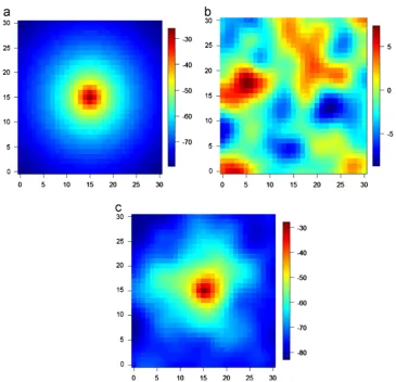
j¼1as the true propaga-tion maps.Fig. 3displays a realization ofδ⋆

j (sampled from

π) and the functions μ⋆

j and F⋆j, defined on the grid C¼ f0;…;30g f0;…;30g. The parameters used in this figure are Oj¼ ð15;15Þ, and c⋆_j, d⋆j and Σ are given in

Section 5. In the sequel, we write

θ⋆def_¼ð

c⋆; d⋆; δ⋆_{; s}⋆;2_Þ; where

c⋆def¼ fc⋆_jgB

j¼1; d

⋆def_¼

fd⋆_jgB_j¼1 and _δ⋆def¼ fδ⋆

jg B j¼1:

For any xAC and any kZ1, the distribution of Yk

con-ditionally to Xk¼x has a density with respect to the Lebesgue measure on RB _{given by g}

θ⋆ðx;YkÞ, where, for

allydef¼

ðy1;…;yBÞARB,

g_θ⋆ðx;yÞ ¼defð2πs⋆;2ÞB=2 ∏

B

j¼1

exp jyjF⋆j;xj2

2s⋆;2

( )

:

In the sequel, we aim at simultaneously estimating the device position andθ⋆_{using the observationsfYkg}

kZ1. For any positive integer n, any observation set ðy1;…;ynÞ

shortly denoted byy1:n, and any parameterθ¼ ðc;d;δ;s2Þ,

the likelihood of the observationsy1:nis given by

L_θðy1:nÞ ¼

def ∑

x1:nACn

νðx1Þg_θðx1;y1Þ ∏

n

k¼2

qðxk1;xkÞgθðxk;ykÞ:

Letnbe a positive integer andY1:n be a set of observations.

The estimator ofθ⋆_{is set as one maximizer of the function:}

θ¼ ðc;d;δ;s2_Þ↦n1_{½log L}

θðY1:nÞþlogπðδÞ: ð5Þ

4. Online estimation procedure

4.1. EM based algorithms to estimate the propagation maps

The EM algorithm is a well-known iterative algorithm to perform maximum likelihood estimation in hidden Markov models [13]. An EM based algorithm can be introduced to maximize (5). Each iteration of this algo-rithm is decomposed into an E-step where the expectation of the complete data log-likelihood (log of the joint distribution of the states and the observations) condition-ally on the observations is computed; and a M-step which updates the parameter estimate. LetY1:nbe a fixed set of

observations andθibe the current map estimate.

(i) The E-step amounts to computing the conditional expectation

QθiðY1:n;θÞ ¼Eθi

1

nlogpθðX1:n;Y1:nÞjY1:n;

ð6Þ

where logp_θðX1:n;Y1:nÞ is the complete data

log-likelihood andEθi½jY1:nis the conditional expectation

givenY1:nwhen the map isθi.

(ii) The M-step computes the new valueθiþ1by choosing

one of the mapsθmaximizing

θ¼ ðc;d;δ;s2_Þ↦Q

θiðY1:n;θÞþn

1_logπðδÞ:

Define, for anyðx;yÞACRB_{and anyjAf1;…;Bg, the vectors}

s1ðxÞ ¼deff1x0ðxÞgx0_AC; s2;jðx;yÞ ¼deff1x0ðxÞyjgx0_AC; s3;jðyÞ ¼defy2j;

where 1x0ðxÞequals 1 ifx¼x0and 0 otherwise. The constanta

being known, the intermediate quantity associated with the model presented inSection 3can be written, up to an additive constant, as

Q_θiðY1:n;θÞ ¼ B

2logs 2 1

2s2 ∑ B

j¼1

f〈S1;F2

j〉2〈S2;j;Fj〉þS3;jg; ð7Þ

where (the dependence onθi,nandY1:nis dropped from the

notation for better clarity)

S1¼ def

Eθi

1

n ∑

n

k¼1

s1ð ÞjXk Y1:n #

; S2;jdef¼Eθi

1

n ∑

n

k¼1

s2;jðXk;YkÞjY1:n

" #

S3;j¼

def1

n ∑

n

k¼1

s3;jð ÞYk:

Therefore, by(7), it is enough to compute_S1,S2;j and S3;j,

1rjrB, to maximize the function θ¼ ðc;d;δ; s2_Þ↦Q

θi ðY1:n;θÞþn1logπðδÞ. The detailed computations to solve

this optimization problem and to obtain the new map estimateθiþ1are given inAlgorithm 1(where1is the vector

of sizejCj where each entry equals 1 and, for any vectorv, diagðvÞis the diagonal matrix with diagonal given byv).

Algorithm 1. Map update.

Require:n,S1,fS2;jgBj¼1,fS3;jgBj¼1. 1:Computation of intermediate quantities

2:forj¼1 toBdo

3: forxACdo

4: Dj;x¼logJxOjJ.

5: end for

6: M0;j¼diagðS1Þþ s 2

nþ1Σ

1_.

7: M1;j¼diagðS1Þ½IjCjM1 0;j diagðS1Þ. 8: M2;j¼IjCjdiagðS1ÞM0;j1.

9: W1;j¼1TM1;j1.

10: W2;j¼1TM1;jDj.

11: W3;j¼DTjM1;jDj.

12: wj¼W1;jW4;jW22;j.

13:end for

14:Parameter update

15:forj¼1 toBdo

16: cj¼wj1½W3;j1TW2;jDTjM2;jS2;j.

17: dj¼wj1½W2;j1TþW1;jDTjM2;jS2;j.

18: δj¼M0;j½S2;jdiagðS1Þðcj1þdjDjÞ.

19: Fj¼cj1þdjDjþδj.

20: s2_¼B1_∑B

j¼1

fFTjdiagðS1ÞFj2ST2;jFjþS3;jg.

21:end for

22:returnθiþ1¼ ðc;d;δ;s2Þ.

This two step process can be repeated until the like-lihood does not improve significantly. However, when the observations are obtained sequentially, this algorithm does not produce a new estimate as new observations are received. The mobile device localization requires an online method which does not store the data and which fre-quently updates the propagation maps.

Online variants of the EM algorithm have been proposed to obtain map estimates each time a new observation is available. In the case of i.i.d. observations, Cappé and Moulines [6] proposed the first EM based online algorithm. This algorithm replaces the exact computation of the sufficient statisticsS1,S2;jandS3;jby a stochastic approximation step.

In the case of hidden Markov models, when both the

Fig. 3.Example ofδ⋆

observations and the states take a finite number of values (resp. when the state-space is finite) an online EM-based algorithm was proposed by Mongillo and Denève[25](resp. by[5]). These algorithms combine an online approximation of the filtering distributions of the hidden states and a stochastic approximation step to compute an online approximation of the sufficient statistics. This has been extended to the case of general state-space models with Sequential Monte Carlo algorithms in Cappé[4], Del Moral et al. [12] and Le Corff et al.[23]. More recently, Le Corff and Fort[21,22]proposed the Block Online EM (BOEM) algorithm in which the estimate is kept fixed as block of observations is received and is updated at the end of each block. See also Andrieu et al.[1] for an overview of online estimation procedures using Sequential Monte Carlo methods.

4.2. Proposed algorithm for online localization in wireless sensor networks

This paper introduces an EM algorithm for online localiza-tion in wireless sensor networks based on the algorithm introduced in Le Corff and Fort [21,22]. Let fτkgkZ1 be a sequence of block-sizes and defineT0¼

def

0 and, for anykZ1,

Tk¼

def ∑k

i¼1τi. Within each block of observations Yk¼

def

YT_kþ1:Tkþ1, the estimate θk is kept fixed and the sufficient

statisticsSk

1,S

k

2;jandS k

3;jare computed sequentially using the

current estimate θk, the observations Yk and τkþ1 as the

number of observations. The superscript k indicates which observations are used in the definition of the statistics. The next parameter estimate θkþ1 is computed when the last

observationYT_kþ1is received usingAlgorithm 1.

Unlike in the traditional EM algorithm where the suffi-cient statistics are computed using forward–backward tech-niques, Cappé[5], Del Moral et al.[12]and Le Corff and Fort [22]proposed to compute the sufficient statistics recursively (i.e. as the observations are received and without any storage). In general state-space hidden Markov models, these online computations are not available in closed form (except in simple models such as linear Gaussian models) and have to be approximated, e.g. using sequential Monte Carlo methods[4,12]. For finite state-space hidden Markov mod-els, the computations can be performed in theory but are computationally too expensive if the number of states is too large (which is the case in our localization framework, see Section 5). Therefore, sequential Monte Carlo methods are used in this paper to localize the mobile.

In this case, the filtering distributionϕt k

on the blockk,

i.ethe distribution ofXT_kþtgivenYTkþ1:TkþtandXTkν, is

approximated by weighted particles fðξi Tkþt;ω

i TkþtÞg

N i¼1 such that

^

ϕktðxÞ ¼ ∑ N

i¼1ω

i

Tkþtδξi_TkþtðxÞ;

whereδ_ξi

Tkþt denotes the Dirac distribution at positionξ i Tkþt.

For allkZ0 andtAf1;…;τkþ1g,fξiTkþtg N

i¼1is a set of possible mobile positions at timeTkþt. At each time step, the new

population of particles is built from the previous population using the bootstrap filter, see Gordon et al.[20]. The Boot-strap filter combines sequential importance sampling and

resampling steps to produce this set of random particles with associated importance weights. Implementations of such procedures are detailed in Cappé[3], Del Moral[11], Cappé et al.[7], and Doucet and Johansen[14].

Online map estimation: We describe here the online approximation on the blockYkof the statisticSk1which is used to compute the map estimate θkþ1 when Tkþ1 is received. The computations for Sk

2;j and S k

3;j follow the

same lines. The rationale to establish this online approx-imation can be found in Del Moral et al. [12]. The first particlesξ0i

,iAf1;…;Ng, are sampled uniformly inC and the first weights are set asωi

0¼N

1

,iAf1;…;Ng:

(i) Setρi

Tk¼0 for alliAf1;…;Ng.

(ii) For alltAf1;…;τkþ1grepeat

(a) For alliAf1;…;Ng,

drawIinf1_;…;Ngwith probabilities

fωℓ Tkþt1g

N ℓ¼1;

sampleξi

Tkþtqðξ I Tkþt1;Þ; set_ωi

Tkþtpgθkðξ i

Tkþt;YTkþtÞ.

(b)

Compute

ρi Tkþt¼

1

ts1 ξ i Tkþt

þt1

t ∑

N

ℓ¼1

ωℓTkþt1qðξ ℓ Tkþt1;ξ

i TkþtÞρ

ℓ Tkþt1

∑N p¼1ω

p Tkþt1qðξ

p Tkþt1;ξ

i TkþtÞ

:

(iii) The approximation ofSk1 on the block Yk is then

given by

^

Sk1¼ ∑

N

i¼1ω

i Tkþτkþ1ρ

i Tkþτkþ1:

(iv) Once these computations are done for each statistic, the estimate θkþ1 is computed by Algorithm 1

applied withS^k1,S^

k

2;j,S^ k

3;jandτkþ1.

The BOEM proposed in Le Corff and Fort [22] also introduced an averaged estimate fθ~kgkZ0 based on a weighted mean of all the sufficient statistics computed in the past. It is proved in Le Corff and Fort[22] that this averaged estimator has an optimal rate of convergence. This can be easily done recursively after the computation of each statistic in step (iii). Step (iii) is then followed by

ðiii0ÞCompute (withS~01¼0)

~ Sk1¼

Tk Tkþ1

~ Sk11þτ

kþ1

Tkþ1

^

Sk1:

And step (iv) is then followed by

ðiv0ÞOnce these computations are done for each statis-tic, the estimateθ~kþ1is computed byAlgorithm 1applied withS~k1,S~

k

2;j,S~ k

3;jandTkþ1.

Localization procedure: At each time step, we compute two estimators of the device position:

the greatest importance weight:

^ Xtdef¼

ξimax

t ; whereimaxdef¼argmaxiωit:

(ii) Averaged algorithm: As the average sequencefθ~kgkZ0 has a better rate of convergence, another particle systemfðξ~it;ω~itÞgis run using only step (ii) (a) above

by replacing θk by θ~k. Then, the estimation of the

device position is set as

~ Xtdef¼_~

ξ~imax

t ; where~imax¼ def

argmaxiω~it:

Other natural estimators of the device position such as the posterior means could be used:

^ Xt¼ ∑N

i¼1ω

i tξ

i

t and Xt~ ¼ ∑ N

i¼1ω~

i tξ~t

i

:

However, we did not observe significant differences between the estimated localization provided by the pos-terior means and by the proposed estimators with both simulated and true data. Moreover, we observed that the bootstrap filter sometimes produces several clouds of particles remote from each other (each of them is con-centrated around local maxima of the filtering distribu-tion). In this case, the proposed estimators offer a better accuracy than the weighted means. Finally, some indoor maps may not be convex such as inSection 5.2. In this case, the weighted means may not belong to the map while the proposed estimators always do.

Stabilization procedure: We add a stabilization step which consists in regularly replacing the original map estimate by the averaged oneðθk’θ~kÞ. This step is needed

to improve the performance of the algorithm as detailed in Section 5.

5. Experiments

5.1. Simulated data

In this section, all experiments are performed on the finite grid C¼ f0;…;30g f0;…;30g. Note that in the following the particles are sampled on the square½0_;30

½0;30before being associated with the corresponding cells in the finite gridC. Each AP is modeled using the same coefficientsc⋆andd⋆:

8j_Af1_;…;Bg; c_j⋆¼ 26 and d⋆_j ¼ 17_:5_:

Σ is a Gaussian covariance function defined byΣðx;x0Þ ¼def

v1nexpðjxx0j2=v2Þ with v1¼10 and v2¼18. General-ities about hyper-parameter determination in spatial data modeling can be found in Cressie[10]. Ferris et al.[17]also describe the determination of the hyper-parameters v1

andv2(whenc⋆j andd⋆j are set to zero). In our case, these

coefficients were calibrated after a measurement cam-paign in the office presented in Section 5.2. The corre-sponding grid stepsize is 1 m. Details about the calibration method for this particular model can be found in Dumont [15, Section 5.1]. This measurement campaign might seem contradictory with our aim to get ride of such a campaign.

However, we use this calibration to find relevant values for the true parametersc⋆_j,d⋆j. We also use this measurement

campaign to estimate the hyper-parametersv1andv2that

characterize the prior distribution of δ⋆_{. Their values}

influence the smoothness of the Gaussian field δ⋆_{. An}

online estimation ofv1andv2could be considered but is

not addressed in this paper. We assess that a partial measurement campaign on a part of the environment only could be sufficient to calibrate them. We can also consider the same values ofv1andv2for different environments so

that v1¼10 and v2¼18 can be used directly and no measurement campaign is needed. The variance of the observation noise iss⋆;2_{¼25 (this value was calibrated by} computing the variance of a set of RSS observations at a fixed position). Thevariance of the transition kernel defined in(2)is chosen such thata¼6.

All runs are started with the same initial estimates:

δ0¼0,s20¼30 and

8jAf1;…;Bg; c0;j¼ 10; d0;j¼ 30:

The number of particles isN¼25 and the initial posi-tion of each particle is chosen randomly and uniformly in

C. The block sizes are given by

8kAN; τk¼10kþ500:

Mapping error: For each mapFj¼μjþδj, the estimation

error is set as the normalized L1 error, such that the

distance of a given mapFjto the true mapF⋆j ¼μ⋆j þδ⋆j is

ϵj¼

def 1

jCjx∑ACFj;xF ⋆

j;x

;

and the error displayed is the mean over all maps:

ϵdef¼1

B ∑

B

j¼1ϵ

j:

Localization error: For a given block fTkþ1;…;Tkþ1g, the localization error is set as the 0.8-quantile of the sample:

To assess the performance of our method we also display the estimated position given with a particle system run with the true mapsF⋆j (i.e. usingθ⋆ instead of θkin

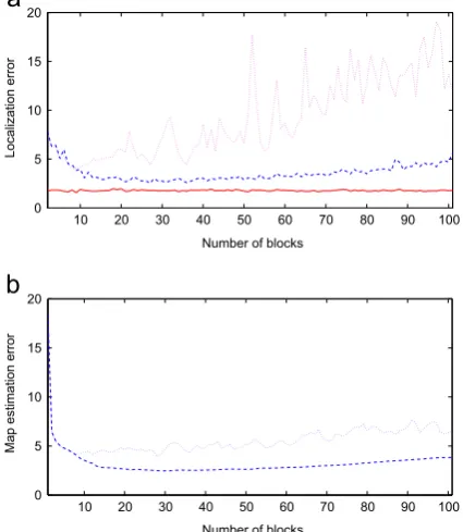
the estimated position does not converge as the number of blocks (i.e. as the number of estimations) increases. After 50 blocks (about 40,000 observations) the position, which is badly estimated, does not provide good map estimates which increases the error on the averaged map estimate. Fig. 5b shows that both the map estimate and its averaged version do not converge. This convergence problem can be due to the curse of dimensionality since the number of parameters to estimate is high. Moreover, the higher the parameter space dimension is, the more likely the EM based algorithms are prone to converge towards local minima (see[7]). To overcome this difficulty, we propose to use the good behavior of the averaged estimate θ~k

which offers a more accurate positioning than the non-averaged version θk (c.f. Fig. 5). Then θk is regularly

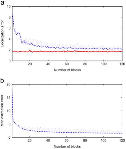
replaced by the averaged version θ~k. In Fig. 6, this

stabilization process is performed each timeNb¼5 blocks

have been used. As shown byFig. 6a and b, this greatly improves the performance of the estimation of the maps and of the localization. Hence, the proposed algorithm uses this stabilization procedure and the averaged esti-mate to localize the mobile.

Figs. 7and8illustrate the performance of the algorithm for the localization and for the estimation of the maps over 50 independent Monte Carlo runs. InFig. 7, the reference localization error (i.e. when the maps are known) is also displayed. The convergence of the localization error to the reference error is almost reached after 100 blocks (about 100,000 observations). Similarly, the error for the estima-tion of the maps given by the averaged algorithm goes on decreasing after 100 blocks (the decrease is slower after 75 blocks).

5.2. True data

In this section, 10 AP are set up in an office environ-ment.Fig. 9represents a map of this environment as well as the position of the AP. The map is discretized using a grid C f0;…;32g f0;…;28g. Note a major difference between the model given inSection 3and the real data situation. For any measure Yk sent by the device, only

several AP are represented in Yk. Therefore, the maps ~

Fj¼μ~jþδ~j are not estimated simultaneously as, for any

time stepk, two AP might appear a different number of times in Y1:k. We thus slightly modify our algorithm by

introducing specific blocks and measure counters relative

0 10 20 30 40 50

3 4 5 6 7 8 9 10

Number of blocks

Localization error

0 10 20 30 40 50

2 3 4 5 6 7

Number of blocks

Localization error

0 10 20 30 40 50

1 2 3 4 5 6 7 8

Number of blocks

Localization error

Fig. 4.0.8-quantile of the distance between the true localization and the estimated position. The localization error is given with the averaged estimate (dotted line) and the reference estimate (bold line): (a) 5 AP; (b) 10 AP; and (c) 17 AP.

10 20 30 40 50 60 70 80 90 100

0 5 10 15 20

Number of blocks

Localization error

10 20 30 40 50 60 70 80 90 100

0 5 10 15 20

Number of blocks

Map estimation error

to each AP. We shortly denote by“jAYk”the fact that APj

belongs toYk.

The variances⋆;2_{is assumed to be known and its value}

ðs⋆;2_{¼25 dBm}2_Þ

is calibrated using a measurement cam-paign at a fixed position. AboutT¼20,000 measures of the RSSI have been made by walking in the office for around 2 h and 45 min with a WiFi connected device (the device measures the RSSI every 0.5 s). Our algorithm produces position estimates however, unlike in the simulated data case, we do not have a direct access to the real position and thus cannot observe the localization error. To

overcome this difficulty, we proceed to four phases of test. During each phase, we regularly identify the true position associated with the last measure. For i in f1;2;3;4g, we denote byStest;i the set of all the time steps belonging to

phasei, and byfXt;YtgtAStest;ithe data collected during this

phase of test. These data will be used to compare the estimated positions fXt~ gtAStest;i with the true positions fXtgtAStest;i. We will also use these data to estimate the

mapping error by considering, for anyj¼ f1;…;10g,

ϵj¼∑

4

i¼1∑tAStest;ijF~j;XtYt;jj1jAYt

∑4

i¼1∑tAStest;i1jAYt

;

where 1jAYt equals 1 if measureYtdoes contain APjand

equals 0 otherwise. Finally, we set

ϵ¼ 1

10 ∑ 10

j¼1ϵ

j:

We run our algorithm twice on the data using the hyper-parametersv1¼10,v2¼18. For these two experiments we will start the algorithm using different initial propagation maps:

F0j;x¼μj0;x¼c0þd0logðJxOjJÞ; jAf1;…;10g;

c0andd0being common to all AP andδ0being set to zero.

In the experiment 1, we consider initial parameters

c0¼ 37 andd0¼ 9 which allow us to start the algo-rithm with initial estimators not too far from the real propagation maps (seeTable 1). In the experiment 2, we choosec0¼ 37 andd0¼9. In this case,d0being positive,

the initial estimators state that the further the device is from an AP, the stronger the signal will be expected. This implies that the experiment 2 starts the algorithm with a completely wrong idea about how WiFi signals propagate in the environment (seeTable 1).

In the two experiments the maps Fj~ ¼μ~jþδ~j were

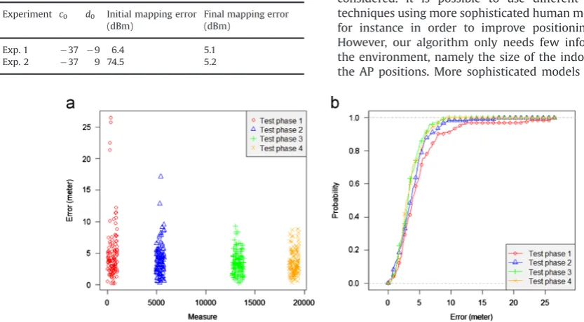
updated a different number of times depending on the AP. This number of updates varies from two times for AP 2 to six times for AP 9. The evolution of the localization precision for the experiment 1 (resp. experiment 2) can be observed inFig. 10(resp.Fig. 11).Figs. 10and11show that the localization improves with time for both experiments. We can observe in Fig. 10 that after a first period of improvement, the precision seems to reach a bound. On the contrary, with the experiment 2, the precision starts

20 40 60 80 100 120

0 2 4 6 8 10

Number of blocks

Localization error

20 40 60 80 100 120

0 5 10 15 20

Number of blocks

Map estimation error

Fig. 6.Map estimation errors and localization errors with the stabilized algorithm: (a) 0.8-quantile of the distance between the true localization and the estimated position with the stabilization process. The localization error is given with the nonaveraged estimate (dotted line), the averaged estimate (dashed line) and the reference estimate (bold line) and (b) mean L1 error on the map estimate with the nonaveraged estimate (dotted line) and the averaged estimate (dashed line) with the stabiliza-tion process.

1 5 10 25 50 75 100

2 3 4 5 6 7 8 9 10

Number of blocks

Fig. 7. Boxplots of the localization error given by the stabilized algorithm with the averaged estimate (left) and the reference estimate (right) as a function of the number of blocks.

1 5 10 25 50 75 100

2 4 6 8 10 12 14 16 18

Number of blocks

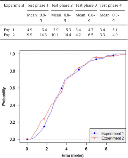
really badly as we expected considering the initial point of our algorithm. The precision seems to stay constant until enough measures have been gathered by the device and until enough updates of the maps have been done. While the precision improves by around 1.5 m between the first test phase and the last one for the experiment 1, for the experiment 2, the precision considerably improves with time with a difference of 6.6 m between the beginning and the end of the experiment (seeTable 2).Fig. 12andTable 2 show that the experiment 2 final precision accuracy reaches (and even slightly overtake) the precision obtained with the experiment 1.

These observations confirm the robustness of our approach. If changes occur in the environment (modifying the way WiFi signals propagate), the difference between the resulting propagation maps and the current estimator will never be as substantial as it was between the true propagation maps and the initial estimate considered in the experiment 2. We reckon that our algorithm can adapt to such changes in order to maintain the accuracy of the localization if the sufficient statistics S~, k and Tk are

regularly reset. Finally, more elaborate localization algo-rithms could be considered to improve the accuracy. However, the aim of this paper lies in the efficiency of our propagation maps estimation procedure for localiza-tion purpose rather than the localizalocaliza-tion algorithm itself.

6. Conclusion

In this paper, we propose an online EM based algorithm to estimate the propagation maps needed in any WiFi based localization system. The main difference with the existing localization solutions is that these propagation maps are estimated using the data sent by the mobile device originally used for localization purposes. The exist-ing WiFi based localization systems establish these propa-gation maps either in a deterministic way or by running a previous hand-made survey. In case of environmental modifications, the propagation maps are changed. Our technique can easily adapt to these changes by regularly reinitializing the estimation procedure while hand-made survey based systems cannot take into account these modifications without renewing the survey. Other ele-ments could be analyzed such as the size of the environ-ment or the materials constituting the obstacles in the environment that might particularly influence the“right choice” of the hyper-parameters v1 and v2. An online

estimation procedure of these hyper-parameters could be considered. It is possible to use different localization techniques using more sophisticated human motion model for instance in order to improve positioning accuracy. However, our algorithm only needs few information on the environment, namely the size of the indoor map and the AP positions. More sophisticated models might need

Fig. 9.Map of the indoor environment with the position of each AP (dots) and their associated identification numbers.

Table 1

c0andd0parameters, initial and final mapping errorsðϵÞ.

Experiment c0 d0 Initial mapping error (dBm)

Final mapping error (dBm)

Exp. 1 37 9 6.4 5.1

Exp. 2 37 9 74.5 5.2

more information and thus make the installation process more complex.

References

[1]C. Andrieu, A. Doucet, S. Singh, V. Tadic, Particle methods for change

detection, system identification and control, Proc. IEEE 92 (3) (2004)

423–438.

[2] P. Bahl, V.N. Padmanabhan, Radar: an in-building RF-based user location and tracking system, in: 19th Annual Joint Conference of the IEEE Computer and Communications Societies, vol. 2, 2000, pp. 775–784.

[3]O. Cappé, Recursive computation of smoothed functionals of hidden

Markovian processes using a particle approximation, Monte Carlo

Methods Appl. 7 (1–2) (2001) 81–92.

[4] O. Cappé, Online sequential Monte Carlo EM algorithm, in: IEEE Workshop on Statistical Signal Processing (SSP), 2009, pp. 37–40.

[5]O. Cappé, Online EM algorithm for hidden Markov models, J.

Comput. Graph. Stat. 20 (3) (2011) 728–749.

[6]O. Cappé, E. Moulines, Online expectation maximization algorithm

for latent data models, J. R. Stat. Soc. B 71 (3) (2009) 593–613.

[7]O. Cappé, E. Moulines, T. Rydén, Inference in Hidden Markov Models,

Springer-Verlag New York Inc., Secausus, New Jersey, USA, 2005.

[8]X. Chai, Q. Yang, Reducing the calibration effort for probabilistic

indoor location estimation, IEEE Trans. Mob. Comput. 6 (6) (2007)

649–662.

[9] Y.-C. Chen, J.-R. Chiang, H.-h. Chu, P. Huang, A.W. Tsui, Sensor-assisted Wi-Fi indoor location system for adapting to environmental dynamics, in: Proceedings of the 8th ACM International Symposium on Modeling, Analysis and Simulation of Wireless and Mobile Systems, ACM, New York, 2005, pp. 118–125.

[10]N. Cressie, Statistics for Spatial Data, Wiley Series in Probability and

Mathematical Statistics: Applied Probability and Statistics, John

Wiley, Hoboken, New Jersey, USA, 1993.

[11]P. Del Moral, Feynman–Kac Formulae: Genealogical and Interacting

Particle Systems with Applications, Springer, New York, 2004.

[12] P. Del Moral, A. Doucet, S. Singh, Forward Smoothing Using Sequen-tial Monte Carlo, Technical Report, 2010,arXiv:1012.5390v1.

[13]A.P. Dempster, N.M. Laird, D.B. Rubin, Maximum likelihood from

incomplete data via the EM algorithm, J. R. Stat. Soc. B 39 (1) (1977)

1–38. (with discussion).

[14] A. Doucet, A. Johansen, A tutorial on particle filtering and smooth-ing: fifteen years later, in: Oxford Handbook of Nonlinear Filtering, 2009.

[15] T. Dumont, Contributions à la localisation intra-muros, de la mod-élisation à la calibration théorique et pratique d'estimateurs (Ph.D. thesis), Université Paris-Sud, Orsay, 2012.

[16]F. Evennou, F. Marx, Advanced integration of WiFi and inertial

navigation systems for indoor mobile positioning, EURASIP J. Appl.

Signal Process. 2006 (2006) 1–12.

[17] B. Ferris, D. Hähnel, D. Fox, Gaussian processes for signal strength-based location estimation, in: Robotics: Science and Systems, The MIT Press, Cambridge, Massachusetts, USA, 2006.

[18]H.T. Friis, A note on a simple transmission formula, Proc. IRE 34 (5)

(1946) 254–256.

[19]J.-M. Gorce, K. Jaffres-Runser, G. de la Roche, Deterministic approach

for fast simulations of indoor radio wave propagation, IEEE Trans.

Antennas Propag. 55 (March (3)) (2007) 938–948.

[20]N. Gordon, D.J. Salmond, A.F.M. Smith, Novel approach to nonlinear

and non-Gaussian Bayesian state estimation, IEE Proc. Radar Signal

Process. 140 (2) (1993) 107–113.

[21]S. Le Corff, G. Fort, Convergence of a particle-based approximation of

the block online expectation maximization algorithm, ACM Trans.

Model. Comput. Simul. 23 (1) (2013) 21–222.

[22]S. Le Corff, G. Fort, Online expectation maximization based

algo-rithms for inference in hidden Markov models, Electron. J. Stat. 7

(2013) 763–792.

Fig. 11.Evolution of the localization precision for experiment 2: (a) tests errors and (b) tests errors CDF.

Table 2

Mean and 0.8-quantile (0.8-q) of the localization errors (in meter).

Experiment Test phase 1 Test phase 2 Test phase 3 Test phase 4

Mean 0.8-q

Mean 0.8-q

Mean 0.8-q

Mean 0.8-q

Exp. 1 4.9 6.4 3.9 5.3 3.4 4.7 3.4 5.1 Exp. 2 9.9 14.3 10.1 14.4 4.2 6.5 3.3 4.9

[23] S. Le Corff, G. Fort, E. Moulines, Online EM algorithm to solve the SLAM problem, in: IEEE Workshop on Statistical Signal Processing (SSP), 2011, pp. 225–228.

[24] D. Madigan, E. Einahrawy, R.P. Martin, W.-H. Ju, P. Krishnan, A. Krishnakumar, Bayesian indoor positioning systems, in: 24th Annual Joint Conference of the IEEE Computer and Communications Socie-ties, vol. 2, IEEE, 2005, pp. 1217–1227.

[25]G. Mongillo, S. Denève, Online learning with hidden Markov models,

Neural Comput. 20 (7) (2008) 1706–1716.

[26]S. Seidel, T. Rappaport, 914 MHz path loss prediction models for

indoor wireless communications in multifloored buildings, IEEE