Original citation:
Ercolani, Nicholas M., Jansen, Sabine and Ueltschi, Daniel, 1969-. (2014) Random
partitions in statistical mechanics. Electronic Journal of Probability, Volume 19 . pp. 1-37.
Permanent WRAP url:
http://wrap.warwick.ac.uk/63577
Copyright and reuse:
The Warwick Research Archive Portal (WRAP) makes this work of researchers of the
University of Warwick available open access under the following conditions.
This article is made available under the Creative Commons Attribution- 3.0 Unported
(CC BY 3.0) license and may be reused according to the conditions of the license. For
more details see
http://creativecommons.org/licenses/by/3.0/
A note on versions:
The version presented in WRAP is the published version, or, version of record, and may
be cited as it appears here.
El e c t ro n ic
J
o f
P r
o
b a bi l i t y
Electron. J. Probab.19(2014), no. 82, 1–37. ISSN:1083-6489 DOI:10.1214/EJP.v19-3244
Random partitions in statistical mechanics
∗Nicholas M. Ercolani
†Sabine Jansen
‡Daniel Ueltschi
§Abstract
We consider a family of distributions on spatial random partitions that provide a coupling between different models of interest: the ideal Bose gas; the zero-range process; particle clustering; and spatial permutations. These distributions are invari-ant for a “chain of Chinese restaurinvari-ants” stochastic process. We obtain results for the distribution of the size of the largest component.
Keywords: Spatial random partitions; Bose–Einstein condensation; (inhomogeneous) zero-range process; chain of Chinese restaurants; sums of independent random variables; heavy-tailed variables; infinitely divisible laws..
AMS MSC 2010:60F05; 60K35; 82B05.
Submitted to EJP on January 7, 2014, final version accepted on September 6, 2014.
SupersedesarXiv:1401.1442v1.
1
Introduction
We study systems of random integer partitions that are independent except for a global constraint on their total mass. Such a setting appears, directly or indirectly, in diverse systems of statistical mechanics: the ideal quantum Bose gas, the zero-range process, particle clustering, certain coagulation-fragmentations processes, and some models of spatial permutations. A common feature is the possibility of a Bose–Einstein condensation; namely, under some conditions, a phase transition takes place that is accompanied with the formation of large objects. In the language of probability, a single random variable realizes the large deviation required to satisfy the constraint on its sum; this behavior is a well-known hallmark for sums of heavy-tailed random variables, and in fact many of our results can be read as abstract results for (conditioned) sums of independent random variables.
We introduce the setting in Section 2. The random objects are “spatial partitions”, that is, collections of integer partitions indexed by locations. The distribution has a product structure subject to a global constraint. Two marginals play an important rôle.
∗Supported by NSF grant DMS-1212167 (N.M.E.), EPSRC grant EP/G056390/1 (D.U.), and ERC advanced
grant 267356 VARIS of F. den Hollander (S.J.).
†The University of Arizona, USA. E-mail:[email protected]
‡Ruhr-Universität Bochum, Germany. E-mail:[email protected]
The first marginal deals with the site occupation numbers; the resulting distribution is that of the ideal Bose gas or of the zero-range process. The second marginal deals with integer partitions; the resulting distribution is that of the particle clustering and of spatial permutations. The present study originated in an attempt at unifying the latter two systems, and the links with the former systems were rather unexpected. It is useful to establish connections since many results and properties of one system can be transferred to the others.
The special cases are described in Section 3. The ideal Bose gas can be found in Section 3.1, the zero-range process in Section 3.2, particle clustering in Section 3.3, coagulation-fragmentations processes in Section 3.4, and spatial permutations in Section 3.5.
The measures considered in this article are invariant measures for interesting Markov processes. One process represents customers in a “chain of Chinese restaurants” which combines the usual Chinese restaurant process with the zero-range process. It is de-scribed in Section 4.1. This actually holds only when the parameters satisfy certain consistency properties. Another process is a coagulation-fragmentation process which is a variant of the Becker–Döring model, see Section 4.2.
The possible occurrence of Bose–Einstein condensation and its consequences are addressed in Section 5. The relevant asymptotic is the thermodynamic limit of statistical mechanics, and the critical density is given by an explicit formula. We study more specific settings in the last two sections, namely, the case of the trap potential in Section 6 and the case of the square potential in Section 7.
2
Random spatial partitions
2.1 Setting
An integer partition1 λof the integer n∈
N is a finite decreasing sequenceλ1 > λ2 > · · · > λk > 1, of varying lengthk, whose elements add up ton: P
k
j=1λj =n;
one often writes “λ` n”. We refer to the lengthk of the sequence as thenumber of componentsof the partitionλ. Every partition is uniquely determined by the numbers rj(λ) = #{i = 1, . . . , k | λi = j}, j ∈N, which count how many times a given integer
jappears in the partitionλ; they are often calledoccupation numbers of the partition. We also define the partition ofn = 0 as the empty sequence (length0, all occupation numbers equal to0).
We are interested in random integer partitions that have additional structure. A spatial partition of the integer n is a collection λ = (λx)x∈Zd of integer partitions at each site x ∈ Zd. That is, eachλ
x is a k-tuple (λx1, λx2, . . . , λxk), wherek varies and
where the integersλxj satisfy
λx1 > λx2 > . . . > λxk > 1 (2.1)
(and we allow for the “empty” sequence withk= 0). The spatial partitionλis uniquely determined by the numbersrxjthat count how many times a given integerj appears in
the partition at sitex,
rxj= #{i= 1,2,· · ·:λxi=j}. (2.2)
We can form two different types of marginals, summing over integersj or sitesx; this gives rise to two different types of occupation numbers. We letr= (rj)j>1denote the sums over all the sites, i.e.,rj =Px∈Zdrxj. The site occupation numbersη= (ηx)x∈Zd are given by
ηx=
X
i>1 λxi=
X
j>1
jrxj. (2.3)
Thus for everyx, λx is a partition of the integerηx. Sometimes this aspect is stressed
and one callsλavector partitionof the vectorη, writtenλ`η(see e.g. [53]).
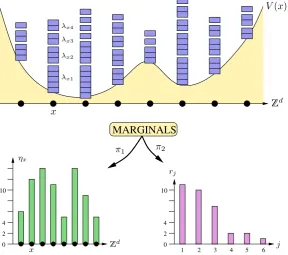
2 0 4 10
MARGINALS
10
0 2 4
1 2 3 4 5 6
Zd j
rj λx1
λx2
λx3
λx4
V(x)
Zd
π1 π2
ηx
x
[image:4.595.152.441.138.393.2]x
Figure 1:A schematic illustration of spatial partitions and the two relevant marginals.
These definitions are illustrated in Figure 1. The intuition is as follows: we think of x∈Zd as sites in space (hence the namespatial partitions). “Space” and “site" should
be taken loosely —xcan be a particle position, a moment vector x = k in a Fourier transformed picture, or a label for an energy level, see the examples and Table 1 in Section 3. LetΛn denote the set of spatial partitions such that
X
x∈Zd,i>1 λxi=
X
x∈Zd, j>1 jrxj=
X
x∈Zd ηx=
X
j>1
jrj =n. (2.4)
In the language of statistical mechanics,Λnis a canonical configuration space with total
particle numbern. Notice thatΛn is a countable set. For later purpose we also define
Nn ⊂ NZ0 as the set of η’s with P
x∈Zdηx = n, and Rn ⊂ NN0 as the set of r’s with P
j∈Nrj =n. Letπ1: Λn → Nn,λ7→r(λ)andπ2 : Λn → Rn,λ7→η(λ)be the natural
projections.
Apart from the space dimensiond, the relevant parameters for our probability dis-tribution onΛn are the following:
(i) A potential functionV :Rd→(−∞,∞].
(ii) A parameterρ∈ [0,∞)which represents the density of the system. We setLd =
n/ρ.
(iii) A sequence of non-negative parametersθ= (θj)j>1.
The probability distribution onΛnis defined as
PL,n(λ) =
1
ZL,n
Y
x∈Zd Y
j>1
1
rxj(λ)!
θj
j e
−jV(x/L) rxj(λ)
The number ZL,n is the normalization; it actually depends onV and θ, but we
al-leviate the notation by neglecting to make it explicit. We assume thatZL,n < ∞ The
relevant asymptotic is the thermodynamic limit where both n and L tend to infinity, withLsuch thatn=ρLd. We will propose different interpretations of the measure
PL,n
later. One such interpretation is that PL,n is a canonical Gibbs measure for particles
moving in the trap potentialV(x/L), forming groups at each site. Particles from dif-ferent groups do not interact; the parameterθj is a Boltzmann weight for intra-group
interactions.2 See Section 3 for details.
2.2 Marginals and conditional probabilities
An advantage of the probability measure (2.5) is that it allows us to switch between random partitions and sums of independent,infinitely divisiblerandom variables. The latter play an important rôle as stationary measures of the zero-range process. These measures arise as marginals ofPL,n.
To be sure, sums of independent random variables, corresponding to the occupa-tion numbersrj, have played a significant rôle in many recent studies of decomposable
random structures (see for instance [6]); but, to the best of our knowledge, this connec-tion to the infinitely divisible random variables, corresponding to the site occupaconnec-tion numbersηx, has not been noticed before. It allows us to deduce limit laws for random
partitions from limit laws for sums of independent variables.
Let PL,n◦π1−1 and PL,n◦π−12 be the push-forwards of PL,n under the projections
ontoNnandRn, respectively. Set
hm=
X
λ`m
Y
j>1
1
rj(λ)!
θj j
rj(λ)
, (2.6)
where the first sum is over the partitionsλof the integerm. We can think ofhmas the
analogue of the normalizationZL,nfor a single site (no product overx, no background
potentialV(x/L)). Later we will discuss the properties of the map(θj)7→(hm).
Proposition 2.1.
(a) The measurePL,n◦π−11 has the product form
PL,n π1−1({η})
=PL,n {λ: η(λ) =η}
= 1
ZL,n
Y
x∈Zd hηxe
−ηxV(x/L). (2.7)
(b) The measurePL,n◦π−12 is of the Gibbs partition form
PL,n π2−1({r})
=PL,n {λ: r(λ) =r}
= 1
ZL,n
Y
j>1
1
rj!
θj j
X
x∈Zd
e−jV(x/L)
rj .
(2.8)
Proposition 2.1 has natural probabilistic proof and interpretation, which we defer to Section 2.4. For now, suffice it to say that the first marginal (2.7) arises as the stationary measure of the zero-range process.
In order to recover the full measure from the marginals, we give below the condi-tional measures PL,n(λ|η(λ) = η)and PL,n(λ|r(λ) = r). Let νm be the measure on
2Our interpretation is consistent with the examples given in Section 3 but different from that of Vershik [53]
and Pitman [49, Chapter 1.5], who consider ZL,n as a microcanonical rather than a canonical partition
integer partitions ofmgiven by
νm(λ) =
1
hm
Y
j>1
1
rj(λ)!
θj j
rj(λ)
. (2.9)
The normalizationhm is defined in (2.6). The measureνmis the analogue of the
mea-sure (2.5) for a single sitex. It is an example of aGibbs random partition which we describe in more details in Section 2.3. The next proposition contains expressions of the conditional probabilities.
Proposition 2.2. The conditional measures are given by
(a) PL,n(λ|η(λ) =η) =
Y
x∈Zd
νηx(λx).
(b) PL,n(λ|r(λ) =r) =
Y
j>1
rj
{rxj}x∈Zd
Y
x∈Zd prxj
xj
, withpxj=
exp(−jV(x/L))
P
y∈Zdexp(−jV(y/L)) .
We leave the elementary proof to the reader. Notice thatPL,n(λ|η)does not depend
onV, andPL,n(λ|r)does not depend on θ. Part (a) says that, conditioned on the site
occupation numbers, the partitionsλx become independent Gibbs partitions. Part (b)
says that givenrj, therxj’s are multinomial: each of therjcomponents of sizejchooses
the sitexwith probabilitypxj.
2.3 Gibbs random partitions
The measureνmdefined in (2.9) can be viewed as describing Gibbs random
parti-tions, which have been studied in detail before, see [6, 34, 16, 33, 48, 55, 45, 47, 25, 7] and Chapters 1.5 and 2.5 in [49]. The main questions deal with the number of elements and their typical size, for given weights (θj). The probability that the typical size is
equal to`is defined by
Pn(X =`) =En
`R` n
=θ`hn−`
n hn
. (2.10)
See Section 5 for more discussion about the random variable for the typical size of elements, where the random element is picked with probability that is proportional to its size.
We now study the relation between the θjs and thehns. This is obviously useful in
view of the relation above. But this relation is also conceptually interesting since the θjs are related to the Lévy measure of a process onN0given by thehns.
Recall that a measure µ is infinitely divisible if for all n ∈ N, there is a measure
˜
µn such thatµ = ˜µn∗ · · · ∗µ˜n is then-fold convolution ofµ˜n. Similarly we say that a
sequence(hm)m>0of non-negative numbers is infinitely divisible if for alln∈Nthere is a sequence ofnon-negative numbers (hm(n)) such that(hm)is the n-fold convolution
of (h(mn))m>0, i.e., h = h(n)∗ · · · ∗h(n). There is a rich theory for infinitely divisible measures [39], closely related to the topic of Lévy processes.
Proposition 2.3. Let(hm)m>0be a sequence of non-negative numbers such thath0=
1and P
mhmz
mhas nonzero radius of convergence. Then there is a unique sequence
(θj)j>1 of real numbers such that Eq. (2.6) holds for allm ∈ N. Moreover, we have θj > 0for allj > 1if and only if(hm)m>0is infinitely divisible.
Proof. We note the power series identity
X
m>0
hmzm= exp
X
j>1 θj
j z
j
(see e.g. [1, Section 3.3]). This identity shows that for a given(hm)there is a unique
sequence of real numbers(θj)such that Eq. (2.6) holds.
Let R denote the radius of convergence of the seriesPh
mzm. Fixz ∈ (0, R), and
let C(z) = P
m>0hmzm and p
(z)
m = C−1hmzm. One can check that (hm) is infinitely
divisible if and only if(pm)is. Furthermore,(p
(z)
m )defines a probability measure onN0 with cumulant generating function
log X
m>0
p(mz)etm= X
j>1 θj
j z
j etj −1
. (2.12)
Here, t satisfies zet < R. We recognize the Lévy-Khinchin representation for an in-finitely divisible measure in the special case of a measure onN0; it follows from clas-sical results (see e.g. Chapter 18 in [39]) that(p(mz))is infinitely divisible if and only if
θj > 0for allj > 1. If this is the case, the weightsα
(z)
j = θj
jz
jdefine a measure on
N, theLévy measure of(p(mz)).
Another question of interest is the relation between the asymptotic behaviors of the sequences(θm)and(hm)asm→ ∞. This has been investigated in the references cited
at the beginning of this subsection. Relevant results can also be found in the probability literature on the relation between the tails of an infinitely divisible measure and its Lévy measure, e.g. in [30, 31]. Here we quote a result of Embrechts and Hawkes [30] on the tail equivalence of an infinitely divisible measure and its Lévy measure; equivalently, on the relation between the tails of(hm)and(θj/j). Recall that the convolution between
two sequences is defined by(a∗b)n=P n
j=0ajbn−j.
Theorem 2.4. (Embrechts and Hawkes [30]) Let(pn)n>0define an infinitely divisible law on N0 with Lévy measure (αj)j>1. Suppose that αj > 0 for all j > 1. Let
αj =αj/(Pk>1αk). The following are equivalent asn→ ∞:
(i) (p∗p)n= 2(1 +o(1))pnandpn+1/pn →1.
(ii) (α∗α)n= 2(1 +o(1))αnandαn+1/αn→1.
(iii) pn= (1 +o(1))αnandαn+1/αn→1.
We note that the Lévy measure of an integer-valued random variable has always finite mass, henceP
j>1αj<∞.
A probability measure onNsatisfying(p∗p)n ∼2pnis calleddiscrete subexponential.
This property suggests that, if two independent variables are conditioned so their sum takes some big value, one variable will take a small value and the other variable will take the appropriate big value. Discrete subexponential variables are necessarily heavy-tailed, that is, P
npnz
n has radius of convergence 1. We can apply this theorem if
P
jθj/j < ∞ and θj+1/θj → 1. Let pm = hmexp(−Pj>1θj/j). The condition (ii)
becomes
n−1 X
j=1 θj
j θn−j
n−j = 2
n/2 X
j=1 θj
j θn−j
n−j = 2 1 +o(1) θn
n X
j>1 θj
j . (2.13)
The first equality is valid ifnis even, there is an unimportant correction in the case of nodd. An immediate consequence of Theorem 2.4 and of the dominated convergence theorem is the following.
Theorem 2.5. Assume thatθn+1/θn →1and thatθn−j/θn 6 cj for1 6 j 6 n2 and
alln, withcjsatisfyingPθjcj/j <∞. Then, asn→ ∞,
hn = 1 +o(1)
θn n exp
X
j>1 θj
j
Notice that cj is necessarily greater or equal to 1, which requires Pjθj/j < ∞.
The theorem was actually proposed in [16] but the connection with infinitely divisible laws and with Theorem 2.4 had not been noticed. It applies in particular to stretched exponential weights,θj/j= exp(−jγ)with0< γ <1.
2.4 Gibbs partitions and Poisson random variables
We conclude this section by explaining in more details the probabilistic picture be-hind Proposition 2.1. To this aim we generalize a well-known relationship between Gibbs partitions and Poisson variables, see for example Eq. (1.53) in [49] or the condi-tioning relation (3.1) in [6].
We assume that there existsz >0such that for allL >0,
X
x∈Zd X
j>1 θj
j z
je−jV(x/L) <∞.
(2.14)
Let(Ω,F,Pz
L)be a probability space and let (Rxj)x∈Zd,j∈N be a family of independent Poisson random variables,
Rxj∼Poiss
θj j z
je−jV(x/L).
(2.15)
Pz
Lis thegrand-canonical measure. The occupation numbers are the random variables
Hx:=
X
j∈N
jRxj, Rj:=
X
x∈Zd
Rxj. (2.16)
We also define the total number of particles by
N = X
x∈Zd X
j∈N
jRxj=
X
x∈Zd Hx=
X
j∈N
jRj. (2.17)
A moment of thought shows that the lawPL,nis recovered by conditioning on the event
P
x,jjRxj=n,
PL,n(λ) =PzL
∀x∈Zd∀j∈
N: Rxj=rxj(λ)
N =n
, (2.18)
and the normalization satisfies
znZL,n=PzL
N=n×exp X
x∈Zd X
j∈N
θj
j z
je−jV(x/L).
(2.19)
Note that in Eq. (2.18) the right-hand side is independent ofz; this is related to the invariance of the measurePL,nunder rescalingsθj →θjzj. Under the measurePzL, the
random variablesRj are independent Poisson variables
Rj ∼Poiss
θj j z
j X
x∈Zd
e−jV(x/L), (2.20)
and theHxare independent variables with cumulant generating function
logEzL
etHx=X
j∈N
θj
j z
je−jV(x/L) ejt−1) (t∈
R). (2.21)
Put differently, Hx is an integer-valued, infinitely divisible random variable with Lévy
measure ν(j) = (θj/j)zjexp(−jV(x/L)), compare with the proof of Proposition 2.3.
Furthermore,
PzL
Hx=m
=hmzme−mV(
x L) e−
P
j>1 θj
j z
jexp(−jV(x/L))
withhmas defined in Eq. (2.6). Indeed,
PzL
Hx=m
= X
λ`m
Y
j>1
PzL
Rxj=rj(λ)
= X
λ`m
Y
j>1
1
rj(λ)!
θj j z
je−jV(x L)
rj(λ)
e−θjj z
jexp(−jV(x L))
.
(2.23)
Proof of Proposition 2.1. For (a), we note that
PL,n π−11 ({η})
=PzL∀x∈Zd: Hx=ηx
N =n
= 1
Pz L(
P
xHx=n)
Y
x∈Zd
PzL
Hx=ηx
(2.24)
and we conclude with Eqs. (2.22) and (2.19). For (b), we observe that
PL,n π2−1({r})
=PzL∀j ∈N: Rj =rj
N=n
= 1
Pz L(
P
jjRj=n)
Y
j∈N
PzL Rj=rj
(2.25)
and conclude with Eqs. (2.21) and (2.19).
3
Relationship with existing models
Our setting is closely related to several models of interest, namely the ideal Bose gas, the zero-range process, particle clustering, coagulation-fragmentation, Becker– Döring, spatial permutations, and population genetics. The relations are explained in this section. Each situation comes with its own language; the keywords and their cor-respondence are summarized in Table 1.
Zero-range particle site -Chinese restaurant customer restaurant table ideal Bose gas, particle Fourier mode, cycle spatial permutation energy level
particle clustering, particle site in space cluster (droplet) nucleation
[image:9.595.92.496.109.378.2]population genetics individual colony same-allele group within colony
Table 1: Language of the different models and their correspondence.
3.1 Ideal Bose gas
Although it was not fully appreciated at the time, Bose–Einstein condensation is the first description of a phase transition in statistical mechanics. The ideal Bose gas is a quantum system whose description involves a complex Hilbert space and the Schrödinger equation; but its equilibrium state is a probability distribution of occupa-tion numbers of Fourier modes. It fits our setting, by choosingV(x) =βkxk2andθ
j≡1;
β is the inverse temperature. With the change of variables k = 2Lπx, writing λkj
in-stead ofλxj,PL,nbecomes a probability measure on spatial partitions(λkj). Summing
occupation numbers
PL,n(π1−1({η})) =
1
ZL,n
Y
k∈2π LZd
e−βkkk2ηk. (3.1)
Summing overk we get that the marginalPL,n◦π2−1 is the probability distribution of cycle lengths associated with the ideal Bose gas [52, 10]. ThusPL,nprovides a coupling
of the distribution of momenta and cycle lengths for the ideal Bose gas. This generalizes to independent bosons in a trap, when the weightexp(−βP
kkkk
2η
k)is replaced with
exp(−βP
r∈IErηr), whereIis a countable index set replacingZdandEr(r∈ I) are the
eigenvalues of the Schrödinger operator in the trap. Results in this case were recently obtained in [20] (see also [18]).
The interacting Bose gas is much more complicated and it does not fit the present setting. But a partial mean-field approach for the dilute regime suggests that interac-tions can be approximated by cycle weightsθj[14].
3.2 Zero-range process
This describes a system of classical particles with stochastic dynamics. There are nparticles moving on the sites{1, . . . , L}and we letη∈ Hn denote the occupations of
the sites. The dynamics is as follows. A particle exits the sitexat rateg(ηx), whereg
is a given functionN →(0,∞), and it chooses a new site uniformly at random among the neighbors. As it turns out, the spatial dimension does not appear in the stationary measure, so the model is usually studied ind= 1. The invariant measure is
PL,n(η) =
1
ZL,n L
Y
x=1
hηx, (3.2)
where the functionhk is related to the ratesgby
hk = k
Y
i=1
1
g(i). (3.3)
It fits the setting studied in this article by choosing the potentialV such that e−V(s) = χ[0,1](s); see Eq. (2.7).
It was noticed by Evans [36] that for certain ratesg, the system possesses a critical density where a sort of Bose–Einstein condensation takes place. See also [41, 5, 4, 22] for further studies. Variants of the model allow for motion on graphs other than Zd
and hopping mechanisms different from the simple random walk, see [36, 54, 40] and the references therein. When e−V differs from the characteristic function, the
marginal (2.7) is the stationary measure of aninhomogeneouszero-range process, com-pare with Eq. (2.4) of [40].
3.3 Particle clustering
The measure PL,n describes approximately the droplet size distributions for a
sys-tem of interacting particles in the canonical Gibbs ensemble, see [51, 43] and the ref-erences therein. Letv be a pair potential with a finite rangeR > 0. Thus particles at mutual distance larger thanRdo not interact. With each configuration (x1, . . . , xn)∈
[0, L]dnwe associate a graph by drawing a line betweenx
i, xjwhenever|xi−xj| 6 R,
and we callNk(x)the number of connected components having kparticles. We have
PN
k=1kNk(x) = n. We put on[0, L]
dn the canonical Gibbs measure at inverse
given droplet size distribution(Nk)becomes approximately n
Y
k=1
1
Nk!
LdZk(β)
Nk
, (3.4)
whereZj(β)is a partition function over droplet-internal degrees of freedom [43]. Eq. (3.4)
corresponds to a measure of the form (2.8) withP
xexp(−V(x/L))replaced byL d, and
θj/j=Zj(β).
3.4 Coagulation-fragmentation processes and Becker–Döring equations
The Becker–Döring system of coupled ordinary differential equations [9] is a popular model for the dynamics of nucleation, with interesting long-time behavior [8]. A natural stochastic variant of the model is the following. Let (aj)j>1 and(bj)j>1 be positive numbers such that for all j, θ1θjaj
j =
θj+1bj+1
j+1 . We define a continuous-time Markov chain with state space{λ: λ`n}and two types of transition:
• Coagulation: a monomer decides to join aj-cluster. The transition(r1, rj, rj+1)→
(r1−1, rj−1−1, rj+1+ 1)happens at rateajr1rj/Ld ifj 6= 1, anda1r1(r1−1)/L2 forj= 1.
• Fragmentation: a monomer decides to depart from a j-cluster, resulting in the transition(r1, rj−1, rj)→(r1+ 1, rj−1+ 1, rj−1). This happens at ratebjrj.
One can check through detailed balance that the marginal (2.8) with the square po-tential exp(−V(s)) = 1[0,1](s) is a stationary measure of this process. The dynamics is a stochastic version of the Becker–Döring equations much in the same way as the Marcus–Lushnikov coalescent is a stochastic version of the Smoluchowski coagulation equations [2]. The model can be easily generalized to allow for joining and departure of groups of size larger than one, and falls into the class of well-studied coagulation-fragmentation processes, see e.g. [29, 12]. In Section 4.2 we propose a “spatial” version of the process for which our measurePL,nis stationary.
3.5 Spatial permutations
Models of spatial permutations are motivated by Feynman’s approach to the Bose gas and by Süt˝o’s work on cycles [52]. A more general framework was proposed in [13], which was studied further in [15, 17]. Spatial permutations involve a distribution jointly over points inRdand over permutations of these points, with penalties that discourage
long jumps. More precisely, the probability space isΛn× S
n, whereΛis the box[0, L]d
(with periodic boundary conditions),nis the number of points, andSn is the group of
permutations ofnelements. Letξ:Rd →[0,∞]and define
ZL,n=
X
σ∈Sn Z
Λn
dx1. . .dxn n
Y
j=1
e−ξ(xj−xσ(j)). (3.5)
The probability element for having pointsx1, . . . , xnand permutationσis then
1
ZL,n
Yn
j=1
e−ξ(xj−xσ(j))
dx1. . .dxn. (3.6)
The marginal obtained after summing over permutations is a permanental point pro-cess, which we do not discuss here despite interest of its own. We rather focus on properties of permutation cycles. We make the extra assumption that e−ξ has
the marginal over the cycle lengths, after integrating over positions and summing over compatible permutations, is precisely the marginal (2.8). This follows from the Pois-son summation formula, see [13] for details. Notice that the special caseξ(x) =βkxk2 corresponds to the homogeneous ideal Bose gas described in Section 3.1.
3.6 Population genetics
Considernindividuals that carry different alleles of a given gene, and live in differ-ent locations orcoloniesx. Inside each colony, we group individuals that carry the same allele. This gives rise to a spatial partition. In the Ewens caseθj ≡θ, one might
imag-ine that our measure is stationary for a population model that includes migration (with some colonies possibly more attractive than others) and mutation. Remember that the Ewens sampling formula appears naturally in the infinite alleles model with mutation rateθ; see [28] and references therein for more background.
4
Stochastic processes
Here we propose two continuous-time Markov processes with state spaceΛn that
havePL,n as a reversible (hence stationary) measure. The first process combines the
zero-range process with the Chinese restaurant process; it has the nice structural prop-erty that the vector of site occupation numbersη(λ(t))is Markovian (regardless of the starting point λ(0)) and evolves as the zero-range process. However we are able to define the Chinese restaurant part only when the weights θj are j-independent. For
non-constantθj’s, we replace the Chinese restaurant step by instant reshuffling. The
second process is a coagulation-fragmentation process that is very natural from the point of view of the Becker–Döring model of nucleation explained in Section 3.4.
4.1 Chain of Chinese restaurants
Recall that, in the Chinese restaurant process, customers enter the restaurant one by one. The(n+ 1)th customer sits next to an existing customer with probability n+1θ, and starts a new table with probability n+θθ. The table occupation is a random partition and the distribution after n customers is given by the Ewens measure. That is, take θj≡θin Eq. (2.9). We refer to Chapter 3 in [49] for background and details.
We adapt the dynamics to spatial partitions as follows. To each site x ∈ Zd is
as-sociated a restaurant. The total number of customers isnand it is conserved. Letηx
denote the number of customers at sitex, andλx`ηxdenote the table occupation. We
consider a continuous-time Markov dynamics where
• A customer exits restaurantxat rateg(ηx); he is chosen uniformly among theηx
customers atx.
• The new restauranty is chosen with probabilityt(x, y). It may depend onL. We assume thatP
yt(x, y) = 1, and that
e−V(x/L)t(x, y) = e−V(y/L)t(y, x). (4.1)
• In the restauranty, the new customer sits next to another customer with proba-bility 1
ηy+θ, and at an empty table with probability
θ ηy+θ.
Withhn defined in (2.6), we take the rate to beg(n) =hn−1/hn(withg(0) = 0). One can
check thathn =θ(θ+ 1). . .(θ+n−1)/n!and thatg(n) = θ+nn−1. A possible choice for
t(x, y)is e−V(y/L)/P
z e
−V(z/L) (withy=xbeing allowed).
unless there existx, y∈Zdandj, k∈
N(withk6= 0) such that
rxj(λ0) =rxj(λ)−1, ry,k+1(λ0) =ryk(λ)−1,
rx,j−1(λ0) =rx,j−1(λ) + 1, ry,k(λ0) =ryk(λ)−1
(4.2)
and all other occupation numbers arerziunchanged. In this case, the rate is
q(λ,λ0) =g(ηx(λ))t(x, y)p−(j, λx)p+(k, λy). (4.3)
Here, the probability that the customer leaving restaurantxleaves aj-table is
p−(j;λx) =
jrxj
ηx
(4.4)
and the probability that the customer joins a k-table (k > 1) or opens a new table (k= 0) is
p+(k;λy) =
kryk
ηy+θ
, p+(0;λy) =
θ ηx+θ
. (4.5)
The stationary measure of this process is precisely the measure defined in Eq. (2.5). Indeed, it satisfies the detailed balance condition.
Lemma 4.1. The rate of Eq. (4.3) satisfies the detailed balance condition
PL,n(λ)q(λ,λ0) =PL,n(λ0)q(λ0,λ).
Proof. We only need to consider the caseλ6=λ0. When the customer changes restau-rants, we have to check that
PL,n(λ)g(ηx(λ))t(x, y)p−(j;λx)p+(k;λy)
=PL,n(λ0)g(ηy(λ0))t(y, x)p+(k+ 1;λ0y)p−(j−1;λ0x). (4.6)
Using (4.1), one can check that for allλ,λ0 and allη, we have the identities
PL,n π−11 ({η})
g(ηx)t(x, y) =PL,n π−11 ({η−δx+δy})
g(ηy+ 1)t(y, x),
νηx(λx)p−(j;λx) =νηx−1(λ 0
x)p+(j−1;λ0x),
νηy(λy)p+(k;λy) =νηy+1(λ 0
y)p−(k+ 1;λ0y).
(4.7)
The detailed balance property now follows from Proposition 2.2.
Since the state space Λn is infinite, we need to check that the Markov process is
non-explosive; to this aim we need the following lemma.
Lemma 4.2. We have
X
λ,λ0∈Λn λ6=λ0
PL,n(λ)q(λ,λ0)<∞. (4.8)
Proof. We have
X
λ0
q(λ,λ0) = X
x,y∈Zd X
j,k∈N
g(ηx(λ))t(x, y)p−(j, λx)p+(k, λy)
=X
x
g(ηx(λ))
=X
x
ηx
θ+ηx−1
6 n
θ.
Defineq(λ,λ) =−P
λ∈Λn,λ06=λq(λ,λ
0)andQ= (q(λ,λ0)) λ,λ0∈Λ
n. For later purpose we note
q(λ,λ) =−g(ηx(λ))
X
y6=x
t(x, y)−g(ηx(λ))t(x, x)
X
k6=j
p+(k;λ−xj). (4.10)
Consider the backward Kolmogorov equations
∂Pt
∂t (λ,λ
0) = QP
t(λ,λ0) =
X
λ00∈Λ
n
q(λ,λ00)Pt(λ00,λ0), (4.11)
with the standard initial conditionP0(λ,λ0) =δλ,λ0.
Proposition 4.3. There is a unique Markov semi-group(Pt(λ,λ0))t>0solving the back-wards Kolmogorov equations for the rates (4.3). It defines a Markov process(λ(t))t>0 with state spaceΛn, which hasPL,nas a reversible (hence stationary) measure.
Note that(Pt)defines a strongly continuous contraction semi-group in`∞(Λn)with
infinitesimal generatorQ:Pt= exp(tQ).
Proof. This follows from Lemmas 4.1 and 4.2, and the non-explosion criterion given in [21], Corollary 3.8.
Proposition 4.4. Let(λ(t))t>0 be the Markov process from Proposition 4.3, with ar-bitrary initial law. Then the marginal(η(λ(t)))t>0is a Markov process with transitions
(ηx, ηy)→(ηx−1, ηy+ 1)(x6=y, all other occupation numbers unchanged) happening
at rateg(ηx)p(x, y).
Hence the site occupation numbers evolve according to a (possibly inhomogeneous) zero-range process; the total rate for a customer to leave a restaurant is g(ηx)(1−
p(x, x)).
Proof. Observe
X
λ0`η0
q(λ,λ0) =g(ηx(λ))t(x, y)
X
j,k
p−(j;λx)p+(k;λy) =g(ηx(λ))t(x, y) (4.12)
ifη0=η(λ)−δx+δy, and in view of Eq. (4.10),
X
λ`η
q(λ,λ) =g(x, ηx)t(x, x)
X
k6=j
p+(k;λ−xj) +q(λ,λ) =−g(x, ηx)
X
y6=x
t(x, y). (4.13)
Letq˜(η,η0) :=g(ηx)t(x, y)ifη0 =η−δx+δy for somex, y∈Zdwithx6=y,q˜(η,η0) = 0
ifη0 6=ηis not of the form just described,q˜(η,η) := 1−P η0∈N
n,η06=ηq˜(η,η
0), andQ˜ := ˜
q(η,η0) η,η0∈N
n. An argument similar to the one used in the proof of Proposition 4.3 shows that P˜t := exp(tQ˜)uniquely defines a Markov semi-group on Nn, which is an
inhomogeneous zero-range process. Eqs. (4.12) and (4.13) become
X
λ0`η0
q(λ,λ0) = ˜q(η(λ),η0) (4.14)
for all λ ∈ Λn, η0 ∈ Nn. The latter identity can be conveniently recast in operator
language: setR(λ,η) :=1{λ`η}=δη,η(λ).We haveQR=RQ, hence˜ PtR=RP˜tfor all
t > 0, i.e.,
X
λ0`η0
Pt(λ,λ0) = ˜Pt(η(λ),η0). (4.15)
This condition is sufficient to ensure thatη(λ(t))t>0is Markovian with transition rates
˜
Thus we have constructed a process combining the zero-range and Chinese restau-rant process for which the measures PL,n are reversible. Finally, let us address the
non-Ewens case where the parameters(θj)depend onj. There exist Markov processes
such that the measure (2.5) is stationary. For instance, take a zero-range process on the
(ηx), together with an “instant reshuffling” of the partitions at the two locations where
a customer has been lost or gained. The transition rate of the process is
g(ηx)t(x, y)νηx−1(λ 0
x)νηy+1(λ 0
y).
One can check that Propositions 4.3 and 4.4 remain true. It would be nice to discover other, more natural Markov processes.
4.2 Coagulation-fragmentation processes
For our second process, let(aj)j>1and(bj)j>2be positive sequences such that for allj,
aj
θj
j θ1=bj+1 θj+1
j+ 1. (4.16)
In addition to (4.1), we assume that for somez >0satisfying Eq. (2.14), we have
X
x,y∈Zd
e−V(x/L)t(x, y)<∞, X
x∈Zd,j>2 bj
θj
j z
je−jV(x/L) <∞.
(4.17)
As the process presented here is a generalization of the stochastic version of the Becker– Döring model presented in Sec. 3.4, we use the vocabulary of nucleation/particle clus-tering and we speak of particles and clusters (or droplets) instead of customers or restaurants.Monomersare clusters of size1. We allow three types of transitions:
• Coagulation at a given sitex: aj-cluster (j > 1) and a1-cluster coagulate to a
(j+ 1)-cluster, i.e.,(rx,j−1, rj,x, rx,j+1)→(rx,j−1−1, rx,j−1, rx,j+1+ 1). This occurs at rateajrxj(λ)rx1(λ)ifj6= 1, and at ratea1rx1(λ)(rx1(λ)−1)ifj= 1.
• Fragmentationat a given sitex: a monomer departs from aj-cluster (j > 2). The transition(rx1, rx,j−1, rx,j)→(rx1+ 1, rx,j−1+ 1, rx,j−1)occurs at ratebjrxj(λ).
• Jump of a monomer from site x to sitey 6= x: the transition(rx1, ry1) → (rx1−
1, ry1+ 1)occurs at raterx1(λ)t(x, y).
There are many possible generalizations: for example, we could allow for the jumping of whole clusters rather than only monomers, or allow two groups of size larger than one to coalesce, or take coagulation-fragmentation rates proportional to powers of the occupation numbersrxjγ , see [29]. We stick to the process presented here for notational simplicity, and also because it is closest in spirit to the original Becker–Döring model of nucleation [9] set in the framework of kinetic gas theory: monomers are mobile particles of a dilute gas, clusters of sizej > 2 are small chunks of condensed precipitate and they are deemed immobile (or at least very slow compared to gas particles).
Proposition 4.5. The transition rates specified above define uniquely a Markov semi-group with state spaceΛn. The measure PL,n is reversible, hence stationary, for the
associated Markov process.
Proof. We leave the proof of the detailed balance conditions to the reader and look at the non-explosion criterion from Lemma 4.2. Letz >0 be such that Eq. (2.14) holds. The contribution to P
monomers is estimated as
X
λ∈∪nΛn
PzL(λ)
X
x∈Zd,j∈N
ajrxj(λ)rx1(λ) = X
x∈Zd,j∈N aj
θ1ze−V(x/L) θj
j z
je−jV(x/L)
= X
x∈Zd,j>1 bj+1
θj+1 j+ 1z
j+1e−(j+1)V x/L) <∞.
(4.18)
We have used that underPz
L theRxjs are independent Poisson variables, and we have
used the assumption (4.16). The contributions of coagulation of monomers, fragmenta-tion, and random walk can be evaluated in a similar way. We conclude as in Lemma 4.2 and Proposition 4.3.
It is natural to ask about the evolution of the marginals η(λ(t)) and r(λ(t)). Let us first look at the site occupation numbers. The rate for a particle to leave a site depends on the number of monomers at this site, i.e., it is not a function of the total number of particles at the site alone. Therefore η(λ(t)) is not Markovian. However, it is natural to approximate the process by replacing the jump rate rx1t(x, y) by the conditional expectation
t(x, y)EL,n rx1(λ)
ηx(λ) =ηx
=t(x, y) X
rx1>1
rx1νηx(rx1) =
θ1hηx−1 hηx
t(x, y), (4.19)
which is the transition rate for a zero-range process (for the last equality, see Propo-sition 2.1 in [33]). Now look at the cluster size counts rj = Pxrxj. Remember
that the conditional law ofrxj is binomial withrj trials and success probability pxj ∝
exp(−jV(x/L)). Again,r(λ(t))t>0 will not be Markovian, but it is natural to approxi-mate it by a process with effective coagulation rate
X
x∈Zd ajEL,n
h
rx1(λ)rxj(λ)
r1(λ) =r1, rj(λ) =rj i
=ajr1rj
X
x∈Zd
px1pxj, (4.20)
forj 6= 1. Similar expressions hold for coagulation of two monomers and for the ef-fective fragmentation rate. In the case of square traps,exp(−V(x/L)) =1[0,L)d(x)with L ∈ N, we have pxj = L−d1[0,L)d(x) and the effective rates are exactly those of the Becker–Döring process from Section 3.4.
5
Condensation
We study the asymptotic behavior in the thermodynamic limitn→ ∞,L→ ∞at fixed densityρ=n/Ld. The model may undergo aphase transitionwhen the density varies.
Above a certaintransition densityρc, acondensationoccurs that is characterized by the presence of large components.
Condensation is measured by the following “order parameters”:
ν∞= lim
K→∞nlim→∞
ρLd=n
EL,n
1 n
X
j>K
j Rj
(5.1)
µ∞= lim
K→∞nlim→∞
ρLd=n
EL,n
1 n
X
x:ηx>K ηx(λ)
. (5.2)
(The existence of the limits overn is proved in the proof of Theorem 5.3 below. The existence of the limits overKis guaranteed by monotonicity.) We say that condensation occurs if µ∞ > 0 or ν∞ > 0, and refer to µ∞ or ν∞ as the condensate fraction. In principle, it might happen thatν∞< µ∞. But Theorem 5.2 below shows thatν∞=µ∞; the two definitions of condensation are equivalent.
Under some assumptions, we prove the existence of a transition densityρcsuch that the order parameters are zero forρ 6 ρcand positive forρ > ρc. In order to define the transition density, let
ρ(z) = X
j>1 θjzj
Z
Rd
e−jV(x)dx. (5.3)
Letzc ∈(0,∞]be the radius of convergence of the power series above. Thetransition density is
ρc=ρ(zc). (5.4)
It is possible thatρcis infinite, meaning that no transition takes place. In the casezc= 1 we get
ρc= X
j>1 θj
Z
Rd
e−jV(x)dx. (5.5)
The transition density may be finite for two reasons (or a combination of both). First, a trap such asV(x) = kxkδ yieldsR
e−jV ∼j−d/δ, which is summable ifδ < d. This
is the case of the ideal Bose gas of Section 3.1, whereθj ≡1 and δ = 2. Eq. (5.5) is
then the famous formula derived by Einstein in 1924. Second, the parametersθj may
be summable. This is the case of the invariant measure of the zero-range process of Section 3.2 in the regime studied by Evans [36]. There is no confining potential here, R
e−jV ≡1. A very different situation is particle clustering, see Section 3.3, where the
parametersθjare given by certain cluster integrals [44]. The general form of (5.3) with
θj 6≡ 1 andV 6≡0 appeared in the context of spatial random permutations with cycle
weights [14, 15] discussed in Section 3.5. A variant of the alternative expression (5.3) for zero-range processes with disorder can be found e.g. in [40] (Eq. (4.2)).
If we are given parameters hn instead of the θj, we can consider the alternative
expression
ρ(z) =
Z
Rd P
n>1nhnzne−nV(x)
P
n>0hnzne−nV(x)
dx, (5.6)
where the integrand is by definition equal to0whenV(x) =∞. Indeed, the right side of Eq. (5.6) is equal to
Z
Rd z ∂
∂zlog X
k>0
hkzke−kV(x)
dx,
and using (2.11) with z 7→ ze−V(x) we get ρ(z) in (5.3). The expression (5.6) is the density-activity series for the (inhomogeneous) zero-range processes.
Assumption 5.1. Assume thatV :Rd →[0,∞]is continuous at0, withV(0) = 0, and
that for everyj > 1, we have
1
Ld
X
x∈Zd
e−jV(x/L) →
Z
Rd
e−jV(x)dx
asL→ ∞.
It follows from this assumption that the series P
j>1
θj
jz
j has the same radius of
convergencezc as the series (5.3) for ρ(z). The next theorem claims thatρc is indeed the transition density.
Theorem 5.2(Condensation). Under Assumption 5.1, we have
ν∞=µ∞= max 0,1−ρρc.
The proof of this theorem can be found immediately after Theorem 5.3 below. It is possible to provide more detailed results about “typical sizes” of components. Choose a customer at random, and consider the size of the element of the partition that he belongs to. Informally, we have
Prob(typical size of element isj)=EL,n
jRj n
. (5.7)
Indeed, there are jRj customers in tables withj people. Similarly, letNk denote the
number of restaurants withkpeople:
Nk(ω) = #{x∈Zd: Hx(ω) =k}. (5.8)
The probability that a random customer finds himself in a restaurant withkpeople is
Prob(typical site occupation isk)=EL,n
Nk n
. (5.9)
The next theorem gives the asymptotic behavior of typical sizes. In order to state it, we introducez0(ρ)as the unique solution of the equationρ(z) =ρwhenρ < ρc; we set z0(ρ) =zcwhenρ > ρc.
Theorem 5.3(Typical sizes). Under Assumption 5.1, we have for allj > 1andk > 0,
(a) jRj n
p
−→ 1 ρθjz0(ρ)
jZ
Rd
e−jV(x)dx,
(b) Nk n
p
−→ 1 ρ
Z
Rd
khkz0(ρ)kexp(−kV(x)) P
j>0hjz0(ρ)jexp(−jV(x))
dx.
Here,−→p denotes the convergence in probability asn, L→ ∞withρLd=n.
The proof of this theorem can be found at the end of the section. We first use it to prove Theorem 5.2.
Proof of Theorem 5.2. We have
ν∞= 1− lim
K→∞L,nlim→∞
K
X
j=1
EL,n
jRj n
= 1−1 ρ
X
j>1
θjz0(ρ)j Z
Rd
e−jV(x)dx
(5.10)
and the definitions ofρc andz0(ρ)imply thatν∞ = max(0,1−ρρc). The proof forµ∞ is
The rest of this section is devoted to the proof of Theorem 5.3. The method relies on the conditioning relation (2.18); we first prove limit laws for the grand-canonical measuresPz
L and then show that the conditioning merely picks the right activity z =
z0(ρ). Technicalities arise because the grand-canonical probability to have exactly n particles goes to 0, and because the power series at finite L need not converge at z=zc.
Lemma 5.4 below and the limit law for theRj’s are closely related to large deviations
results [11, 52, 10, 41, 44]; we provide a complete proof because our setting is more general.
Lemma 5.4.
lim
n→∞
ρLd=n
1
nlogZL,n=
1
ρ X
j>1 θj
j z0(ρ)
j
Z
Rd
e−jV(x)dx−logz0(ρ).
Proof. Using Eq. (2.19) but neglecting the probability term, we get
1
LdlogZL,n 6
X
j>1 θj
j z
j 1
Ld
X
x∈Zd
e−jV(x/L) −ρlogz. (5.11)
For anyz < zc, we have by dominated convergence
lim sup
n→∞
ρLd=n
1
Ld logZL,n 6
X
j>1 θj
j z
j
Z
R
e−jV(x)dx−ρlogz. (5.12)
The bound extends toz=zcby continuity. The equation of Lemma 5.4 holds at least as an upper bound.
For the lower bound, we start with Proposition 2.1 (b). We have
ZL,n > n
Y
j=1
1
rj!
θj j
1
Ld
X
x∈Zd
e−jV(x/L)
rj
(5.13)
for any choice of non-negative integers(rj)such thatPjrj =n. Let us introduce the
following entropy function on sequencesa= (aj)such thataj > 0andPjjaj 6 1:
I(a) =−X
j>1 ajlog
eθj jajρ
Z
Rd
e−jV(x)dx. (5.14)
We have
1
nlogZL,n > −I 1
nr1,
1
nr2, . . .
+X
j>1 rj
n log 1
Ld P
x∈Zd e−jV(x/L) R
Rd e−jV(x)dx −1
n
n
X
j=1
log rj! (rj/e)rj
.
(5.15)
Letaj be equal to the right side of Theorem 5.3 (a). We choose a sequencer(n)such
thatPjr(n)
j =n,
1
nr
(n)
j 6 2aj, and n1r
(n)
j →aj asn→ ∞. By continuity ofV around0,
we have
constj−d 6 Z
e−jV(x)dx 6 Z
e−V(x)dx,
constj−d 6 1 Ld
X
x
e−jV(x/L) 6 1
Ld
X
x
e−V(x/L) 6 const,
(5.16)
then use the dominated convergence theorem and the first sum in Eq. (5.15) vanishes in the limitn→ ∞. The last sum also vanishes: Using1 6 rj!
(rj/e )rj 6 Crj, we have for anyK
1
n
K
X
j=1
log rj! (rj/e )rj 6
1
n
K
X
j=1
logCn, (5.17)
which goes to 0 asn→ ∞. Further, usinglogs 6 s,
1
n
n
X
j=K+1
log rj! (rj/e )rj 6
1
n
n
X
j=K+1
logCrj 6
C K
n
X
j=K+1 jrj
n 6 C
K. (5.18)
This is arbitrarily small by choosingKlarge enough. Finally, recall thatIis continuous on the set of non-negative sequences(bj)satisfyingPjbj 6 1[8]. Then
lim inf
n→∞
1
nlogZL,n > −I(a), (5.19)
and a calculation shows that−I(a)is equal to the right side of the expression in Lemma 5.4.
Recall the definition ofEz
Lgiven in Section 2.4.
Lemma 5.5. For anyz < zc, we have
(a) lim
L→∞E
z L
jRj Ld
=θjzj
Z
Rd
e−jV(x)dx.
(b) lim
L→∞E
z L Nk Ld = Z Rd
hkzke−kV(x)
P
j>1hjzje−jV(x)
dx.
Proof. We have
EzL
jRj Ld
=θjzj
1
Ld
X
x∈Zd
e−jV(x), (5.20)
and the limit (a) exists by Assumption 5.1. For the limit (b), we have
EzL
Nk Ld = 1 Ld X
x∈Zd
hkzke−kV(x/L)
P
jhjzje−jV(x/L)
= 1
Ld
X
x∈Zd
hkzke−kV(x/L) exp
n
−X
j
θj
j z
je−jV(x/L)o.
(5.21)
We can expand the last exponential so as to get a convergent series of terms of the form
e−nV(x/L) withn∈
N. The Riemann sums converge in the limitL→ ∞by Assumption 1, and the result follows from dominated convergence.
Lemma 5.6. Letz < zcanda >0. There existL0andb >0such that for allL > L0, we have
(a) PzLL1d
Nk−EzLNk
> a
6 e−bLd,
(b) PzLL1d
Rj−EzLRj
> a
Proof. We bound the cumulant generating functions and then deduce bounds with the help of Markov’s inequality. Since random variables at different locations are indepen-dent, we have
1
LdlogE z L
et(Nk−EzLNk)= 1 Ld
X
x∈Zd
logEzLhexpt1{Hx(ω)=k}−tP
z
L(Hx=k)
i
= 1
Ld
X
x∈Zd n
−tPzL(Hx=k) + log
1 + ( et −1)PzL(Hx=k)
o .
(5.22)
Usinglog(1 +s) 6 s, we find
1
Ld logE z L
et(Nk−EzLNk)
6 et −1−t 1 Ld
X
x∈Zd
PzL(Hx=k)
= et −1−t
EzL
Nk Ld
.
(5.23)
The latter expectation converges by Lemma 5.5 (b) so that everything is bounded by c(z)t2fort
6 1withc(z)depending onzonly. Then
PzL
1
Ld(Nk−EzLNk)> a
=PzLet(Nk−EzLNk) > etaLd
6 e−taLdEzLet(Nk−EzLNk)
6 e−Ld(ta−c(z)t2).
(5.24)
This is smaller than12e−bLd for someb >0. A similar bound can be found forPzL(L1d(Nk−
Ez
LNk)<−a)and this completes the proof of (a). The same method can be used to prove
the claim (b) forRj.
Proof of Theorem 5.3. We only prove the claim (b), as the proof for (a) is the same. Let mk be the limit in (b). We have
PL,n
NLkd −mk
> ε
6 PL,n
NLkd −E
z L(
Nk
Ld) > ε−
mk−EzL( Nk
Ld) = P z L
NLdk−EzL( Nk
Ld) > ε−
mk−EzL( Nk
Ld) Pz L P
j>1jRj =n
.
(5.25)
Then
PzL
X
j>1
jRj =n
=znZL,nexp
n
− X
x∈Zd X
j>1 θj
j z
je−jV(x/L)o.
(5.26)
We choosezclose toz0(ρ)in such a way that
mk−
Z
Rd
hkzke−kV(x)
P
j>1hjzje−jV(x)
dx 6 ε 2, X
j>1 θj
j z
j
−z0(ρ)j) Z
Rd
e−jV(x)dx−ρlog z
z0(ρ) 6 a 2. (5.27)
(Ifρ < ρc, we can choosez=z0(ρ); ifρ > ρc, we need to choosezclose enough tozc.) From Lemma 5.6 there existb >0andL0such that for allL > L0, we have
PzL
NLdk−E
z L(
Nk
Ld) > ε−
mk−EzL( Nk
Ld)
It follows from Lemma 5.4 that there existsL1such that ifL > L1, we have
PzL
X
j>1
jRj=n
> e−aLd. (5.29)
Choosinga < b, we get the claim.
6
Trap potentials
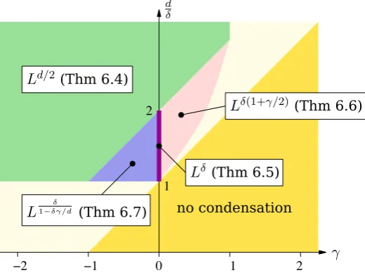
In this section we investigate the shape and location of the condensate for a class of potential functions that have a unique minimum at the origin; square traps are treated in Section 7. Theorem 6.2 states that the condensate is located at the origin (the trap’s minimum), and Theorems 6.4–6.7 provide the fluctuations of the occupation of the ori-gin. The fluctuations are governed by infinitely divisible laws that need not be normal orα-stable, as expected for sums of independent random variables that are not identi-cally distributed [39]. Theorems 6.2, 6.4 and 6.5 generalize known results [15, 18, 20], Theorems 6.6 and 6.7 are new. A graphical overview is given in Figure 2. Section 6.3 discusses the distribution of the partition elements at the origin: the condensate can concentrate on a single large element or be distributed according to some non-trivial law, e.g. a Poisson-Dirichlet distribution.
6.1 Macroscopic occupation of the origin
In this subsection we consider the marginal measure onηand we establish that the excess mass is concentrated atx= 0. We also prove a central limit theorem.
Assumption 6.1. We assume that the potential functionV : Rd →[0,∞]satisfies the following properties:
(i) V(x) =kxkδ(1 +o(1))around the origin with0< δ < d.
(ii) V(x)> b >0for allkxk>1.
(iii) For everya >0, there exists a constantCa such that
1
Ld
X
x∈Zd\{0}
e−aV(x/L) < Ca
Z
Rd
e−aV(x)dx <∞;
we also assume that the left side converges toR
e−aV asL→ ∞.
For the weights, we assume thatθj >0for allj, thatlimj→∞1jlogθj= 0, and that
X
j>1 θj
jd/δ <∞. (6.1)
Notice that ifV(x)≈ckxkδwithc >0around the origin, there is no loss in generality
in takingc = 1. Indeed, let L0 = c−1/δL and V0(x) = V(c−1/δx). Then V0(x) ≈ kxkδ
around 0 and the probability can be written in terms ofL0andV0by replacing e−jV(x/L) by e−jV0(x/L0).
It follows from our assumptions thatRRdexp(−jV(x))dxis bounded from above and below by a constant times j−d/δ, whence z
c = 1 and ρc < ∞. Additional regularity conditions on theθjs, formulated as conditions on the tails of thehns, will be imposed in
the theorems. They are loosely related to regularity conditions for heavy-tailed random variables [31] and can be checked, in part, with the help of Theorem 2.5.
condensate to a single site; in fact the limitδ→ ∞corresponds, formally, to the square traps from Section 7, where all sites are alike and the condensate chooses uniformly among them. It is not clear how largeδshould be in order for this to occur.
Recall thatH0is the random variable for the total occupation of the origin.
Theorem 6.2. Suppose that Assumption 6.1 holds true, and that there exist constants C, c > 0anda 6 12(1−δ
d)such that for alln > 1,
C−1e−cna 6 hn 6 Cecn
a .
Assume also thatρ > ρc. Then asn, L→ ∞with fixedρ=n/Ld, we have the conver-gence in distribution
1
LdH0
d
−→ρ−ρc.
The theorem applies to algebraically decaying weights θj = j−γ, γ > 0, by
Theo-rem 2.5. It also applies to stretched exponential weightsθj/j= e−j
γ
and algebraically growing weightsθj=jγ withγ >0small enough. In the latter case, we indeed have
hn= 1 +o(1)
cn−(γ+2)/[2(γ+1)]expCnγ/(1+γ) (6.2)
for suitable constantsc, C. Eq. (6.2) was proven by Erlihson and Granovsky, see Eq. (4.66) in [34]. It also follows from results proven independently in [33]. (The proof in [33] was given for specific weights that satisfyθj= (1 +o(1))jγ, but it can be extended
with the help of known results on polylogarithms [37, Chapter VI.8].)
For the proof of Theorem 6.2 we follow [18, 15], see also [20]. First we express the canonical expectations with respect to the grand-canonical measure atz =zc = 1 with the help of the conditioning relation (2.18). A difficulty here is thatP
jθj/j can
be infinite, in which casePzc
L(H0 =∞) = 1. Therefore we give a special treatment to x= 0. Let
M(ω) = X
x∈Zd\{0}
Hx(ω) =
X
j>1 X
x∈Zd\{0}
jRxj(ω) (6.3)
be the number of particles not at0.3 LetρL
c = 1
LdE
zc
L(M); this is approximately equal to
the critical density:
ρLc = 1
LdE zc
L(M) =
1
Ld
X
j>1 X
x∈Zd\{0}
θje−jV(x/L), (6.4)
which converges toρc by dominated convergence.
Lemma 6.3. Under the same assumptions as in Theorem 6.2, there existC, c >0such that for allL >0and allB >0,
Pzc
L
L1dM−ρ
L
c > B
6 Cexp(−c B L(d−δ)/2.
If in additionP
jjθj/jd/δ <∞, the same estimate holds with exponentmin(d/2, d−δ)
instead of(d−δ)/2.
As we shall see later, the additional condition means thatM has normal fluctuations of orderLd/2; if the confining potential is quite shallow, δ > d/2, our large deviations estimate kicks in at fluctuations of the order ofLδ only.
3A careful inspection of the definitions shows that the measureµ
Λused by Buffet and Pulé [18] and Betz
and Ueltschi [15] is, in our notation, the law ofMunderPzc
L. The variableMis also used by Chatterjee and
Proof. Recall that the cumulant generating function of a Poisson variableN ∼Poiss(λ)
islogEetN =λ( et −1). Lett=t
L∈Rwitht2L=O(Ld−δ). We have
logEzc
L
etL(Ld1 M−ρLc)= X
j>1 X
x∈Zd\{0}
logEzc
L
ejtLLd1 (Rxj(ω)−EzLcRxj)
= X
j>1 X
x∈Zd\{0} θj
j e
−jV(x/L) ejtL/Ld −1−jtL Ld
.
(6.5)
Using|es −1−s| 6 1 2s
2e|s|, the interior sum is bounded by
1 2θj
1
Ld
X
x∈Zd\{0}
e−12jV(x/L) hjt2
L
Ld e
−j(1
2V(x/L)−Ld1 tL) i
. (6.6)
Because of Assumption 6.1 (i), there exists b0 >0 such thatV(x/L) > b0L−δ for all
non-zerox∈Zd. Sincet
LLd−δ, the square bracket is bounded, for largeL, by
jt 2
L
Ld exp −
b0
4Lδj
6 t
2
L
Ld ×
4Lδ
b0e. (6.7)
Then there is a constantC0>0such that
logE zc L
etL(Ld1 M−ρLc) 6 C
0 t2L
Ld−δ
X
j>1 θj
jd/δ =O(1). (6.8)
Using Markov’s inequality,
Pzc
L
1
LdM−ρ
L
c > B
6 e−tLBEzc
L
etL(Ld1 M−ρLc), (6.9)
and a similar bound for the probability that L1dM −ρLc 6 −B (use a negativetL).
IfP
jjθj/jd/δ<∞, we choosetL=O(Ld−δ)to bound the square bracket in (6.6) by
a constant timesj. The right side in (6.8) is then replaced byconst(t2L/Ld)P
jθj/jd/δ
and it is bounded whentL=O(Ld/2).
Proof of Theorem 6.2. We have
Pzc
L
Xn
j=1
jR0j=`
=h`exp
− n X j=1 θj j (6.10) so that
PL,n(H0=`) =
Pzc
L(
Pn
j=1jR0j =`)PLzc(M =n−`)
Pzc
L(
Pn
j=1jR0j+M =n)
, (6.11)
EL,n
et(n−H0)= E
zc
L[hn−Me tM]
Ezc
L[hn−M]
. (6.12)
We use the convention thathm= 0whenm <0.
We show thatEL,n
exp(Ltd(n−H0))
→ etρc for anyt. Convergence in distribution follows from the pointwise convergence of the Laplace transform and we get the claim of the theorem. It is enough to show that for anyε >0, we have
Ezc
L[hn−M1|M/Ld−ρL c|>ε]
Ezc
L[hn−M]
We have
Ezc
L[hn−M1|M/Ld−ρL c|>ε]
Ezc
L[hn−M] 6
maxj6nhj
minj6nhj
Pzc
L(|
1
LdM−ρ
L
c|> ε)
Pzc
L(M 6 n) 6 maxminj6nhj
j6nhj
Ce−cεL(d−δ)/2.
(6.14)
The last inequality follows from Lemma 6.3. The last term vanishes indeed as L → ∞.
6.2 Fluctuations of the condensate
We now study the fluctuations of the condensate. The goal is to find the correct scalingαand the limiting random variableX such that
H0−Ld(ρ−ρLc) Lα
d
−→X. (6.15)
For simplicity, we fix the potentialV(x) =ckxkδ in this subsection. It turns out that the
phase diagram of the fluctuations is very rich. It is pictured in Fig. 2. We only provide partial results, see the regions in dark colors. The lightly colored region is left to future studies; it would certainly be interesting to know what happens there.
0 2
1
−2 −1 1 2
no condensation
γ
d δ
L
δ(Thm 6.5)L
1−δγ/dδ (Thm 6.7) [image:25.595.167.427.372.571.2]L
δ(1+γ/2) (Thm 6.6)L
d/2 (Thm 6.4)Figure 2: Phase diagrams of the fluctuations of the condensate for the weightsθj = jγ and the potentialV(x) =ckxkδ
. Results for the dark regions are stated in Theorems 6.4 to 6.7. For d
δ 6 γ+ 1, there is no condensation. The light region remains to be investigated.
The first result deals with normal fluctuations. Let
σc2= X
j>1 jθj
Z
Rd
e−jV(x)dx. (6.16)
The first result holds in the case where the variance above is finite.
Theorem 6.4 (Central limit theorem for H0). Assume that V(x) = kxkδ, ρ > ρc and P