warwick.ac.uk/lib-publications
Original citation:
Ba, Dang Xuan, Dinh, Quang Truong and Ahn, Kyoung Kwan. (2016) An integrated intelligent
nonlinear control method for a pneumatic artificial muscle. IEEE/ASME Transactions on
Mechatronics, 21 (4). pp. 1835-1845.
Permanent WRAP URL:
http://wrap.warwick.ac.uk/87074
Copyright and reuse:
The Warwick Research Archive Portal (WRAP) makes this work by researchers of the
University of Warwick available open access under the following conditions. Copyright ©
and all moral rights to the version of the paper presented here belong to the individual
author(s) and/or other copyright owners. To the extent reasonable and practicable the
material made available in WRAP has been checked for eligibility before being made
available.
Copies of full items can be used for personal research or study, educational, or not-for profit
purposes without prior permission or charge. Provided that the authors, title and full
bibliographic details are credited, a hyperlink and/or URL is given for the original metadata
page and the content is not changed in any way.
Publisher’s statement:
“© 2016 IEEE. Personal use of this material is permitted. Permission from IEEE must be
obtained for all other uses, in any current or future media, including reprinting
/republishing this material for advertising or promotional purposes, creating new collective
works, for resale or redistribution to servers or lists, or reuse of any copyrighted component
of this work in other works.”
A note on versions:
The version presented here may differ from the published version or, version of record, if
you wish to cite this item you are advised to consult the publisher’s version. Please see the
‘permanent WRAP URL’ above for details on accessing the published version and note that
access may require a subscription.
Abstract—This paper proposes an advanced position tracking
control approach, referred to as an integrated intelligent nonlinear controller (IIN), for a pneumatic artificial muscle (PAM) system. Due to the existence of uncertain, unknown, and nonlinear terms in the system dynamics, it is difficult to derive an exact mathematical model with robust control performance. To overcome this problem, the main contributions of this work are as follows: i) to actively represent the behavior of the PAM system using a grey-box model, neural networks are employed as equivalent internal dynamics of the system model and optimized online by a Lyapunov-based method; ii) to realize the control objective by effectively compensating for the estimation error, an advanced robust controller is developed from the integration of the designed networks and improvement of the sliding mode and backstepping techniques and iii) the convergences of both the developed model and closed-loop control system are guaranteed by Lyapunov functions. As a result, the overall control approach is capable of ensuring the system’s performance with fast response, high accuracy, and robustness. Real-time experiments are carried out in a PAM system under different conditions to validate the effectiveness of the proposed method.
Index Terms—Pneumatic artificial muscle, backstepping
control, sliding mode control, integrated control, neural network, online identification.
NOMENCLATURE
ˆ
Estimate of.
ˆ
Estimation error of *, ,
Maximum and minimum values of *.
sup
Supermen absolute value of. Approximated error of the function.
Range width of *.
x Position of the PAM (mm). d
x Desired position of the PAM (mm).
x
Velocity of the PAM (mm/s). p Pressure inside the PAM (bar).2, 3
Positive learning gains. 2, 3
Positive estimation error gains.
2, 2, , .3 3 |
j j f g f g
Q Positive-definite diagonal gain matrices. 1, 2, i2, 3, i3
k k k k k Positive control gains.
2, 3
Positive integrated gains.
Manuscript received September 13th, 2015. This work was supported by the 2015 research fund of University of Ulsan, S. Korea.
Dang Xuan Ba is with the Graduate School of the Mechanical Engineering, University of Ulsan, S. Korea (e-mail: [email protected]).
I. INTRODUCTION
HE outstanding development of robotics in recent decades has resulted in requirements for various actuators. For compliant applications or rehabilitation robots, pneumatic artificial muscle (PAM) actuator represents a feasible solution due to many advantages of cleanliness, safety, low cost, light weight, high force/volume ratio, and force/weight ratio. Some remarkable applications of PAM actuators include therapy machines [1]-[2], wearable robots for the treatment of ankle injuries [3], limb exoskeletons [4], and parallel manipulators [5]. First proposed by McKibben in the 1950s for orthotic and prosthetic applications, the actuator is simply structured from a contraction system and fitting connections at the end points. The contraction system consists of an inner inflatable rubber hose and a covering of loose-weave fibers. By applying a strong enough pressure, the muscle shortens and generates a contraction force along the axial direction. The generated force depends on the strength of the applied pressure. The presence of various uncertain, nonlinear, and unknown terms within the device makes difficulties in deriving an accurate model as well as designing an effective tracking controller for the actuator.
To model PAM dynamics, numerous approaches have been developed in recent years. In mathematical methods [6]-[8], the static and dynamic characteristics of PAMs were derived from the physical analysis of pressure-force relationships, geometric structure, contraction ratios, elastic characteristics, and viscous and Coulomb frictions. The results showed that the actuators were hard to accurately describe using these models. Thus, a number of experimental approaches have been conducted to obtain more accurate PAM dynamics [9]-[12]. Though the dynamics have been estimated from empirical data and successfully applied to position control, the wide-spread applicability of these methods is limited. Recently, another category of PAM modeling methods based on intelligent techniques has been proposed to achieve better performance. Previously [13]-[14], the system dynamics were represented by a black-box model using a nonlinear auto-regressive exogenous (NARX) fuzzy configuration and were then optimized by basic or modified genetic algorithms. Although the modeling effectiveness was clearly improved, some disadvantages were still observed. For instance, the training process was attempted
Dinh Quang Truong is with WMG, University of Warwick, United Kingdom (e-mail: [email protected]).
Kyoung Kwan Ahn is with the school of the Mechanical Engineering, University of Ulsan, S. Korea. (Corresponding author; phone: +82-52-259-2282; fax: +82-52-259-1680; e-mail: [email protected]).
Dang Xuan Ba, Truong Quang Dinh, and Kyoung Kwan Ahn,
Member, IEEE
An Integrated Intelligent Nonlinear Control
Method for Pneumatic Artificial Muscle
offline using input/output data and the models were hard to combine with a model-based controller. Thus, it is necessary to develop a flexible model that can represent the behavior of PAM actuators and supply sufficient information to develop a position controller.
From the PAM control perspective, a number of approaches have been proposed to deal with the challenges of this actuator type. A PID controller for a six degree-of-freedom (DOF) robotic arm driven by PAM actuators was structured from the mathematical model of the system dynamics [15]. An extended PID controller was developed based on experimental modeling of the actuator [16]. Through the good control results, the effects of these methods were proven. Nevertheless, due to the high nonlinearity and sensitivity to the working conditions of PAM systems (for example, supplied pressure, temperature, or viscosity), the applicability of such controllers is limited only to a specific region. To increase the control performance by covering the uncertain and nonlinear terms of PAM systems, advanced robust adaptive approaches have also been exploited based on the mathematical models. The system dynamics were represented by linear models in which the system parameters were identified through experimental measurements and were then used to construct the controllers [17]-[21]. Although better results were achieved, employing linear models in the controller design for high nonlinear plants such as PAM actuators certainly restricts the control efficiency. To overcome this problem, a nonlinear model incorporated with an adaptive fuzzy controller [22] was used to obtain higher control accuracy. Nonetheless, neglecting the pressure dynamics can lead to degradation of the control effect in different working conditions. In [23]-[25], the nonlinear models were derived more comprehensively than in [22] to exactly describe the system behavior. After validating the control results, the author confirmed that the control efficiency was not maintained even for the same type of actuators. Hence, adaptive models were employed to develop the controllers in which the system uncertainties were identified online by the least-squares (LS) methods [26]-[27]. The control performances were further increased using these approaches. However, unmodeled and unknown terms were not still covered by the controllers. To solve these issues of the model-based approaches, intelligent methods have been developed, such as neural network-based control [28]-[30], fuzzy PD+I learning control [31], advanced intelligent nonlinear PID controllers [32]-[34], hybrid fuzzy-neural control [35], tuning fuzzy controllers [36]-[38], and switching predictive approaches [39]. Here, the control objective was realized by utilizing neural networks or fuzzy schemes to represent the system behaviors as black-box models or to adjust the control parameters via various learning algorithms such as back propagation (BP), recursive least squares (RLS), or bumpless transition (BT) mechanisms. Hence, the problem of unknown or hard-to-model terms was addressed. In fact, because most of the PAM applications are used for therapy or nursery tasks, maintaining the stability of the closed-loop system is very important [40]. This issue is hard to resolve by typical intelligent approaches.
In this article, an extended study of the advanced intelligent
control category with a so-called “integrated intelligent nonlinear controller” (IIN) for position tracking control of a PAM system is proposed. The key features of this control approach are as follows:
1) To properly represent the uncertain, nonlinear, and unknown terms of the PAM system and to provide a feasible framework for developing a position controller, neural networks are proposed as equivalent internal dynamics based on a grey-box model and their parameters are then optimized by a Lyapunov-based method.
2) To realize the control objective by actively compensating for the estimation error, a robust controller is designed from the approximation results with the following improvements: - To minimize the design procedure, the structure of the controller is an advanced combination of the sliding mode and backstepping schemes.
- To improve the control efficiency by reducing the steady-state tracking error and avoiding the chattering problem described previously ([20], [38]), integral terms of the state control errors and linear robust functions are appropriately employed. - To increase the excitation ability of the optimization process, the developed networks are integrated into the controller.
3) Lyapunov stability laws are adopted to guarantee the convergences of both the model optimization and the closed-loop performance.
As a result, the design method can ensure good tracking performance with fast response and high robustness for the PAM system. In order to verify the designed IIN controller, a PAM test rig was set up for a comparative study with tracking control. Then, real-time experiments with different testing and loading conditions were performed. The results are discussed to clearly evaluate the control efficiency.
PAM
M
g
Steel spring
b) Mechanical design of the proportional valve MPYE-5-1/8-LF-010B. Fig. 1. Configuration of the studied system.
II. PROBLEMSTATEMENTANDGREY-BOXMODEL In this section, the PAM dynamics are considered as grey-box models in which their detailed structures are unknown and their effective inputs are known. The studied system was set up as shown in Fig. 1(a). It consists of a PAM actuator (MAS-10-N-176-AA-MCFK, Festo), a steel spring, and a load. One end of the PAM is fixed to the frame and the other end is connected to the load-spring system through a disk. The system performance represented by the disk displacement is driven by the PAM, while the spring acts as an antagonistic component. The motion of the actuator is adjusted by a proportional 5-port/3-position pneumatic valve (Series MPYE-5-1/8-LF-010-B, Festo) [41] as shown in Fig. 1(b).
By applying Newton’s second law and previous results ([7], [8], [18], [30]), the force dynamics of the system can be presented under a simple form as
2
( , )
2( )
x f x x
g x p
(1)where f2 is a grey-box function with two inputs (the system positionxand velocity
x
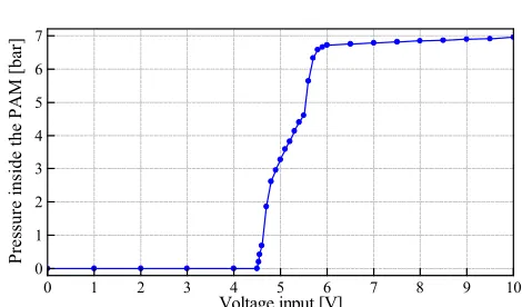
), and g2 is another positive grey-box function of the system position.Figures 1(a) and 1(b) show that, at the same time, the system flow is charged from port 1 to port 4 and is discharged from port 4 to port 5. The opening area from port 1 to port 4 is enlarged with the increase of the valve control input while, inversely, the opening area from port 4 to port 5 is reduced. A numerical investigation of the static flows through the ports used to drive the PAM and the static pressure of the open-loop system with respect to the input voltage was carried out and the obtained results are shown in Fig. 2. It is noted that the total effective opening area of the valve port is driven by the applied voltage (control inputu). The valve characteristics shown in Fig. 2 point out that the dead-zone phenomenon is very small and can be eliminated. From the literature review ([24], [27], [37]), the pressure dynamics of the system can be then derived as follows:
3
( , , )
3( , )
p f x x p
g x p u
(2)where f3 is a grey-box function of the inputs ( , , )x x p andg3
is a positive grey-box function of the inputs ( , )x p .
Remark 1: The spool dynamics of the studied valve are ignored. Based on previous studies [7], [8], [22], [27], [30], it can be seen that the system dynamics (Eqs. (1) - (2)) are not only nonlinear functions of the inputs ( , , )x x p and certain elements such as the relative mass and string stiffness, but they also contain uncertain parameters which are difficult to be determined or may change during the working process, such as the elastic modulus of the PAM rubber, thickness of the rubber sleeve,
friction coefficient, initial braiding angle, supply pressure, temperature, and unknown terms.
0 1 2 3 4 5 6 7 8 9 10
-200 -150 -100 -50 0 50 100 150 200
From Port 1 to Port 4 From Port 5 to Port 4
F
lo
w
[l
pm
]
Voltage input [V]
4.5 5.0 5.5 6.0 -20
-10 0 10 20
(a) Static flow characteristics of selected valve ports.
0 1 2 3 4 5 6 7 8 9 10
0 1 2 3 4 5 6 7
P
re
ss
ur
e
in
si
de
th
e
P
A
M
[b
ar
]
Voltage input [V]
(b) Static pressure characteristics of the open-loop system. Fig. 2. Static flow and pressure characteristics of the system.
III. SYSTEMDYNAMICSESTIMATION
To deal with the difficulty of the representation of uncertainties, nonlinearities, and unknown terms in the system dynamics, in this section, neural networks are properly constructed to approximate the internal functions
f g f2, , ,and2 3 g3
of the grey-box model derived in SectionII.
We define the state variables as follows:
1 2 3
T T
X x x x x x p (3)
As a result, the system dynamics now become
2 2 1 2 2 1 3 3 3 1 2 3 3 1 3
( , ) ( ) ( , , ) ( , ) .
x f x x g x x
x f x x x g x x u
(4)
Assumption 1: The input signaluand state vectorXare bounded and measurable. The internal functions
2( , ),1 2 2( ), ( , , ),and1 3 1 2 3 3( , )1 3
f x x g x f x x x g x x are bounded as
well. Thus, the system described by Eq. (4) is open-loop stable.
[image:4.595.311.546.255.393.2]( )
T
zW
(5)where( )
1 2 ... l
Tis the hidden neural matrix and
1 2 ...
T lWW W W is the constant weight matrix of the output layer that satisfies the following condition:
sup ( ) sup with ( 0).
z z
T
z z
z W (6)
Note that if the functions zand ( ) are bounded, thenW is also bounded.
Based on these assumptions, model (4) can be rewritten as
2 2 2 2 2 2
3 3 3 3 3 3
2 1 2 1 3 3
3 1 2 3 1 3
( , ) ( )
( , , ) ( , )
T T
f f g g f g
T T
f f g g f g
x W x x W x x x
x W x x x W x x u u
(7)
where
f2, g2, f3,and
g3 are bounded.Proposition 1: In order to estimate the unknown functions of the given system, an approximation system is proposed as follows:
2 2 2 2
3 3 3 3
2 1 2 1 3 2 2 2
3 1 2 3 1 3 3 3 3
ˆ ˆ
ˆ ( , ) ( ) ( ˆ )
ˆ ˆ
ˆ ( , , ) ( , ) ( ˆ )
T T
f f g g
T T
f f g g
x W x x W x x x x
x W x x x W x x u x x
(8)
which satisfies the following conditions:
2, 2, ,3 3
ˆ , ˆ,
T T
j j j j j f g f g
W W W W
X X X X
(9) where
2, , ,2 3 3 |
j j f g f g
W are network parameters.
Proposition 2: From the given system described by Eq. (4) and the approximation system (8), the learning laws of the network parameters are proposed as follows:
2 2 2 2 2 2
3 3 3 3 3 3
2 2 2 2 2 2
3 3 3 3 3 3
1
1 2 2 2 1
1 2 3 3 3 1
1 2 2 3 1
1 3 3 3
ˆ ,
ˆ , ,
ˆ ( )
ˆ ,
f f f f e f f
f f f f e f f
g g g g e g g
g g g g e g g
W Q x x e S
W Q x x x e S
W Q x e x S
W Q x x e u S
(10)
where eej j| 2,3 xj xjxˆj.
2, 2, ,3 3 |
j j f g f g
are the diagonal matrices of the boundary-guarantee functions that are defined as
2, 2, , .3 3 1 ( )
1 ( )
1 1 ( ) ( )
| ... ... ... ... ... ... j j j j
j j j f g f g j jk j length W
j jk j length W
j j jk jk j length W j length W
S diag r r r
diag s s s
diag r s r s r s
(11) with
min min max max
ˆ
1... ( ); ;
min max 2 max min
min max min max
if ( ) ( )
1 otherwise where
( )( )
1 ; 0
( )
[ ; ]and ((2 ) 0) .
j jk
jk jk
jk jk k length W b W
b W b W
jk jk
jk
cond
r s
b b b b
b b
cond b b b b b b s
(12)
To verify the convergence of the estimation method, the following theorem is studied.
Theorem 1: Given a grey-box system (Eq. (4)) satisfying Assumptions 1and2 and employing a neural-network model (Eq. (8)) with the learning rules given by Eq. (10), if groups of the constant vectors
2, 2, ,3 3 |
j j f g f g
W exist and the estimating
state errors are sufficiently rich, i.e. 2 2 3 2
2
| | f g x
x
and 3 3 3 3
| | f g u
x
, in transient time, then the approximation model will converge to the system model with an allowable accuracy.
Proof:
Consider the following Lyapunov function:
2 2 3 3
2 2
1 2 2 3 3
, , ,
1 1 1
( ).
2 2 2
T j j j j f g f g
V x x W Q W
(13)We differentiate the candidate function with respect to time and note that Eqs. (4) and (8) lead to
2 2 3 3
2 2 2 2 3 3
3 3
2 2 3 3
1 2 2 2 2 3 3 3 3 3
2 2 1 2 1 3 3 3 1 2 3
1 3 , , , ( ) ( ) ( , ) ( ) ( , , ) ˆ ( , ) ( ).
f g f g
T T T
f f g g f f
T T
g g j j j
j f g f g
V x x x x x u
x W x x W x x x W x x x
W x x u W Q W
(14)Employing the learning laws (Eq. (10)) yields
2 2
3 3
1 2 2 2 2 3
3 3 3 3
( )
( ).
f g
f g
V x x x
x x u
Thus, Theorem 1 is proven.
Remark 2: The magnitudes of the bounds j |j f g f g2, , ,2 3 3
depend on the design of the hidden matrices
j j f g f g| 2, , ,2 3 3. In order to reduce these magnitudes, the matrices are designed to cover the whole working range of the system and to be sensitive to changes of the system variables. Moreover, the larger time derivative of state variables and larger 2, 3 values increase the convergence rate of the identification method. Nevertheless, in real-time applications, choosing very big values for these factors could cause the identification to diverge. Thus, these values should be assigned proper large values.IV. INTEGRATEDINTELLIGENTNONLINEARCONTROLLER DESIGN
In this section, the state-based control method is designed for position tracking of the studied system. The proposed networks are also integrated into the controller in order to enrich the excitation signal of the learning process. The control algorithm is structured from a combination of state stabilities, linear robust functions, and offset cancellation terms.
We define a sliding surface as
1
s k e e (16)
where e x x d is the tracking error.
Differentiating the surface with respect to time and noting Eq. (4) lead to
1 d 2 2 3.
s k e x f g x (17)
Proposition 3: In order to control the surface to be as small as possible, a state control signal is proposed as
3 1 2 2 2 2
2
1 ˆ ˆ
( )
ˆ
v d i i
x k e x f k g s k s
g
(18)
where si is an integral function ofs.
Note that the s e x, ,d terms can be measured. The following
relationship is thus obtained:
3 3 ˆ2 2 ˆ2 2
(xvx ),(f f ) and (g g ) s s. Here, sis a small boundary.
We consider a state control error as
3 3 3v.
e x x (19)
By applying the system (Eq. (4)), the time derivative of the error can be expressed as follows:
3 3 3 3v.
e f g u x (20)
Proposition 4: The final control input is designed such that the state control error can be stabilized within its defined bound, as follows:
2
3 3 3 3 3 3 3 2
3 3
1 ˆ ˆ ˆ
( )
ˆ v i i
u x f k g e k e g s
g
(21)
where ei3is an integral function ofe3.
The designed control inputs always contain estimates of the internal functions which can be calculated from the neural networks presented in Section III. However, the excitation signals of the learning laws depend only on the system states. The learning process may turn off in the case of an insufficiently rich trajectory.
Proposition 5: To increase the enrichment of the excitation signals, the learning laws are improved as follows:
2 2 2 2
3 3 3 3
2 2 2 2
3 3 3 3
1
1 2 2 2 2 1
1 2 3 3 3 3 3 1
1 3 2 2 2 1
1 3 3 3 3 3
ˆ ( , )( )
ˆ ( , , )( )
ˆ ( ) ( )
ˆ ( , ) ( )
f f f f e
f f f f e
g g g g e
g g g g e
W Q x x e s
W Q x x x e e
W Q x x e s
W Q x x u e e
(22)
Theorem 2: Given a bounded grey-box system (Eq. (4)) satisfying Assumptions 1 and 2 and employing the neural-network model (Eq. (8)) and control laws (Eqs. (18) and (21)) with the learning rules improved as described by Eq. (22), the following statements will hold:
a. If the estimating state errors and the state control errors are sufficiently rich, i.e.
3 3 3
2 2
3 3 3
2 2
2 3
2 3
3
2 2 3 3
| | ,| | ,
| | and | |
ˆ ˆ
2 2
f g
f g
f g f g
u x
u x
x x
s e
k g k g
in transient time, then the approximation model will converge to the system model with an allowable accuracy. b. Choosing the positive constants k k k k k1, ,2 i2, ,3 i3, 2, 3
appropriately, the tracking control error of the closed-loop system will converge to a given bound.
Proof:
For any bounded set { :y y y y }, there exists an equivalent set as follows:
{ : and| | }.
2 2
y
y y
(23)
2 2
3 3
2 3 2 2
3 3 3
f g f g x u (24) where 2 3 2 2 2 2 3 3 3 3
and | |
2 2
and| | .
2 2 (25)
The following new Lyapunov function is considered:
2 2 2 2
2 1 2 3 3 2 2
2 2 3
3 3 3 3
1 1 1
( )
2 2 2
1 ( ) . 2 i i i i i i
V V s e k s
k k e k (26)
Differentiating the candidate function (Eq. (26)) with respect to time and employing Eqs. (17) and (21) yield
2 1 2 2 2 1 2 3 3 3 3 1 2 3 2 2 2 1 3 2 2 2 3 2
2
3 3 3 3 1 3 3 3 3 2 3
3 ( , ) ( , , ) ˆ ˆ ( ( ) ) ˆ ˆ ( ( , ) ) T T
f f f f
T g g
T g g
V V sW x x e W x x x
s W x x k g s g e
e W x x u k g e g s
(27)
wheresi s andei3e3.
Combining the results of Theorem 1 and the improvement (Eq. (22)), the following inequality is obtained:
2 2 2 2 2 3 3 3 3 3 3 2 2 2 2 2 3 3 3 3 3
ˆ ˆ
( ) ( )
( ) ( ).
V s k g s e k g e
x x x x
(28)
Hence, the first statement of Theorem 2 is proven. From Eq. (28), we obtain
2 2
3 3 3
3
2 2 2 2 2 2 2
2
3 3 3 3
3 3 3
ˆ
( ) min ,| |
4
min ,| | min ,| | .
ˆ
2 8 4
V s k g s x
e x k g (29)
Therefore, we have the following limitation:
2 2
2 2 2
1 2 2 2 2 2 2 2
1 | |
ˆ 4 ˆ
ˆ
16 e
k k g k g k g
(30) where 3 3 2 2 3 3 3 3 3 3 2 2 2 3 3 3
min ,| |
ˆ
2 8
min ,| | 4
min ,| | . 4 e k g x x (31)
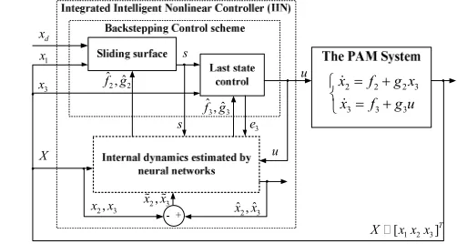
Consequently, the second statement of Theorem 2 is proven. Remark 3: As seen in the proof of Theorem 2, the effectiveness of the designed controller depends not only on the estimation results and control parameters, but also on the other state control errors. Moreover, by adopting the integral terms, the offset control errors are significantly compensated for. A diagram of the proposed controller is illustrated in Fig. 3. A procedure to select suitable parameters of the designed controller is briefly described as follows. In Step 1, the learning
gains
2, 2, 3, 3, 2, 3, 2, 3
f g f g
Q Q Q Q are tuned by the trial-and-error method in order to obtain the best estimation errors based on Eqs. (8) and (10) throughout open-loop experiments. The obtained gains are then used to construct the closed-loop control in Step 2. Next, the main control parameters
k k k1, ,2 i2, ,k k3 i3
are manually chosen for the best controlobjective in both transient and steady-state responses in Step 3. The integrated parameters
2, 3
are tuned to further improve the control performance in Step 4. In the last step, the control result is evaluated: IF it satisfies the desired performance, THEN stop the tuning process, ELSE return to Step 3.2 2 2 3
3 3 3
x f g x
x f g u
d x
1 2 3
[ ]T
X x x x
1
x
3
x
2, 3
x x x x 2, 3 x xˆ ˆ2, 3
2 2
ˆ ˆ,
f g
3 3
ˆ ˆ,
[image:7.595.292.543.477.611.2]f g s 3 e s u u X
Fig. 3. Diagram of the proposed control algorithm.
V. EXPERIMENTALRESULTS
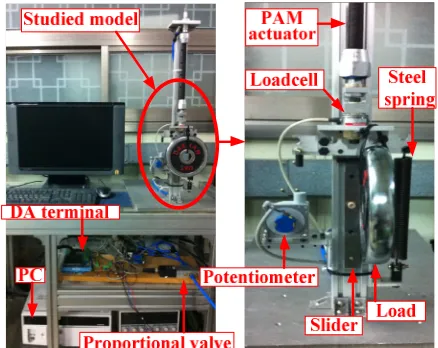
velocity and acceleration were indirectly measured by filtered backward differentiation of the position with a cut-off frequency of 31.8 Hz [24], [43]. In addition, a load cell and an indicator were used to measure the system force. The proposed controller was implemented on the PC within the Matlab/Simulink (Version R2009b) environment combined with the Real-time Window Target Toolbox with a sampling time of 10 ms. This sampling time was chosen based on the bandwidth of the used valve ([41], [44]) and the ability to obtain an acceptable control result. The Bogacki-Shampine method was selected as the solver for the differential equations. Detailed specifications of the experimental devices are listed in Table I, and a photograph of the system apparatus is shown in Fig. 4.
First, the proposed identification method was evaluated by using open-loop experiments. From the system inputs
x x, and p
, there were four internal functions
f x x g x f x x p2( , ), ( ), ( , , ),and ( , ) 2 3 g x p3
that needed to beestimated by the neural networks. Five Gaussian functions were designed to cover the feasible working range of each input. The structure of the hidden layer of each network was then built as a combination of these Gaussian functions with all of the respective inputs and a bias value of 1.
The working ranges of the system were determined as follows:
[ 13;12] mm, [ 100;100] mm/s, [0; 7]bar, and [ 5;5]V.
x x
P u
Here, to easily represent the valve acting direction, an offset value (5 VDC) was added to the control input to convert the valve driving voltage range from [010](VDC) to the control input range of [-55](VDC).
TABLEI
DETAILEDSPECIFICATIONS OFEXPERIMENTALDEVICES
Device Description
PAM
Type: Festo MAS-10-N-176-AA-MCFK Nominal length: 176 mm
Inside diameter: 10 mm Max pressure: 8 bar
Proportional valve Type: Festo MPYE-5-1/8-LF-010-B Max pressure: 10 bar
DAQ card ADVANTECH PCI-1711 AI and AO: 12 bits in resolution
Load cell BONGSHIN CDFS Capacity: 30 kg
Potentiometer Type: CELESCO SP1-12 Input resistance: 10K Ohm Moving bar Weight: 0.61 kg
Spring Static stiffness: 2.607 N/mm
Fig. 4. Photograph of the experimental apparatus.
A random signal to drive the proportional valve was selected as the input for the open-loop identification process. The learning rate matrices and other gains were chosen as
1 1 1
2 26 2 6 3 126
1
3 26 2 3 2 3
12.5 ; 30.26 ; 20.65 ; 19.6 ; 0.12; 0.15; 150; 135.
f g f
g
Q I Q I Q I
Q I
The designed Gaussian functions, the input signal, and the results obtained by applying the algorithm described in Section III to the open-loop system are presented in Fig. 5. As can be seen, despite containing large slopes, the estimated velocity and pressure still converged to the indirectly measured velocity and pressure with small errors (5 mm/s ~ 5.71% of the velocity error and0.2 bar ~ 5.68% of the pressure error). Moreover, the approximation functions are the bounded curves. The ranges of
2( , ), 2( ), ( , , ),3 3( , )
f x x g x f x x p g x p were determined to be [-25; 10], [1; 5], [-4.5; 4], and [2; 7.5], respectively. Note that these functions did not tend to drift away from their own ranges. These results imply that the proposed algorithm is definitely stable.
Next, the integrated controller was implemented on the testing system for position control based on the theory presented in Section IV. The results achieved in the open-loop experiments were used to set the initial values of the controller. The reference trajectories were sinusoidal signals with different frequencies (0.05, 0.5, 1, 1.5, and 0.2 Hz) with/without loading (3, 5, and 7 kg) and a smooth multi-step signal. In addition, to evaluate the designed controller more carefully, a conventional PID controller and an adaptive recurrent neural network (ARNN) controller were applied to the same system for comparison. The respective PID control gains for different properties of the experiments were derived by the trial-and-error method, as displayed in Table II. The ARNN controller was designed based on previous work [29]. The remaining parameters of the IIN controller were selected as follows:
1 2 2
3 3 2 3
100; 2.1; 0.035;
0.38; 0.022; 0.2; 2.5.
i i
k k k
k k
Case study 1: In this case, the control experiments were carried out on the system for tracking the sinusoidal trajectory with amplitude of 10 mm and a frequency of 0.05 Hz in the free-load condition.
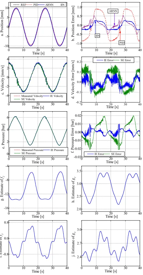
Applying the PID, ARNN, and proposed control methods in turn, the experimental results were obtained and compared as shown in Fig. 6. By employing the PID controller with a fixed gain use, the tracking result was obtained with a 9% control error (±0.9 mm). The ARNN method combined a PID controller and a neural network to enhance the control performance. Here, the network took part in inverse model-based control while the PID functioned as a compensator to maintain the tracking error within an acceptable range. Thus, better performance with a 5% (±0.5 mm) control error was accomplished by using the ARNN. The proposed control idea proved to be the best comprehensive approach. The reason is that the IIN architecture includes the advantages of the backstepping and sliding mode techniques as well as the necessary improvements. As a result, the figure shows that higher control accuracy (±0.25 mm ~ 2.5%) was achieved by the proposed approach. The effectiveness of the estimation idea was also demonstrated through the obtained data. The system velocity and pressure were estimated quite accurately with estimation errors of ±0.1 mm/s and 0.015 bar, respectively, while the internal dynamics
f x x g x f x x p2( , ), ( ), ( , , ), and ( , ) 2 3 g x p3
were approximatedas curves, in turn, within ranges of [-14; 5], [2.1; 3.5], [-1; 0.6], and [2.4; 3.2]. Compared to the separated estimation (SE) method described in Section III, the estimation errors of the integrated estimation (IE) method were clearly improved.
Case study 2: Comparative experiments in the free-load condition were carried out with a smooth multi-step tracking reference within the range of [-10; 10] mm and the results are depicted in Fig. 7. Although the PID controller can work well for a nonlinear system, good performance is normally limited only to a specific region [15], [16]. As seen in the figure, this controller drove the system most accurately at the 3 mm set point. At the other set points, the PID performance was degraded due to the fixed gain use. This disadvantage could be resolved by the ARNN controller by using the network to compensate for the nonlinearities and unknown terms. Consequently, the number of good working regions was clearly increased. However, due to the slow adaption of the ARNN, there were still some large steady-state errors in the tracking results. The figures suggest that the transient response and steady-state behavior of the system using the proposed method were improved as compared to those using the PID and ARNN controllers. This comes as no surprise due to the advanced design of the IIN in which the control performance is enhanced by the integral terms of all concerned state errors, the adaptation laws via the online estimation method with initial parameters well determined from the open-loop experiments.
TABLEII
TUNEDPIDGAINSFORRESPECTIVEEXPERIMENTS
Case Trajectory PID Gains
KP KI KD
Case 1
Sin 0.05Hz-10mm 10 4.5 0.10 Free-load
Case 2
Smooth multi-step 8.5 3.2 0.40 Free-load
Case 3 Sin 10mm
0.5 Hz 13.7 1.3 0.21
1Hz 11.1 1 0.20
Free-load 1.5Hz 9.2 0.7 0.25
Case 4-1
Sin 0.2Hz-5mm 10.2 1.5 0.11 Free-load
Case 4-2 Sin 0.2Hz-5mm
9.8 0.5 0.15
Loading Load 3kg
Case 4-3 Sin 0.2Hz-5mm 9.2 0.7 0.22 Loading Load 5kg
Case 4-4 Sin 0.2Hz-5mm 8.7 0.2 0.07 Loading Load 7kg
0.0 0.5 1.0
min i x
a.
G
au
ss
ia
n
fu
nc
ti
on
s
xi ximax 0 5 10 15 20 25 30
-5.0 -2.5 0.0 2.5 5.0
b.
In
pu
tS
ig
na
l[
V
]
Time [s]
0 5 10 15 20 25 30 -80
-40 0 40
80 Measured VelocityEstimated Velocity
c.
V
el
oc
it
y
[m
m
/s
]
Time [s] 0 5 10 15 20 25 30
-6 -3 0 3 6
d.
V
el
oc
ity
E
rr
or
[m
m
/s
]
Time [s]
0 5 10 15 20 25 30 -20
-10 0 10
e.
E
st
im
at
e
of
f2
Time [s] 0 5 10 15 20 25 30
0 2 4
f.
E
st
im
at
e
of
g2
Time [s]
0 5 10 15 20 25 30 0
2 4 6
8 Measured PressureEstimated Pressure
g.
P
re
ss
ur
e
[b
ar
]
Time [s] 0 5 10 15 20 25 30
-0.3 0.0 0.3
h.
Pr
es
su
re
E
rr
or
[b
ar
]
Time [s]
0 5 10 15 20 25 30 -4
-2 0 2 4
i.
E
st
im
at
e
of
f3
Time [s] 0 5 10 15 20 25 30
2 4 6 8
j.
E
st
im
at
e
of
g3
0 10 20 30 40 -10
-5 0 5
10 REF PID ARNN IIN
Time [s] a. Po si tio n [m m ]
0 10 20 30 40
-1.0 -0.5 0.0 0.5 1.0 Time [s] b. Po si ti on E rr or [m m ] PID ARNN IIN
0 10 20 30 40
-4 -2 0 2 4
Measured Velocity IE Velocity SE Velocity c. V el oc it y [m m /s ]
Time [s] 0 10 20 30 40
-0.2 -0.1 0.0 0.1
0.2 IE Error SE Error
d. V el oc ity E rr or [m m /s ] Time [s]
0 10 20 30 40
0 2 4 6
Measured Pressure IE Pressure SE Pressure e. P re ss ur e [b ar ]
Time [s] 0 10 20 30 40
-0.03 -0.02 -0.01 0.00 0.01 0.02
IE Error SE Error
f. P re ss ur e E rr or [b ar ] Time [s]
0 10 20 30 40
-16 -12 -8 -4 g. E st im at e of f2
Time [s] 0 10 20 30 40
2.0 2.5 3.0 3.5 h. E st im at e of g2 Time [s]
0 10 20 30 40
-0.8 0.0 0.8 i. E st im at e of f3
Time [s] 0 10 20 30 40
[image:10.595.55.290.87.538.2]2.4 2.7 3.0 j. E st im at e of g3 Time [s] Fig. 6. Experimental data with respect to case study 1.
0 5 10 15 20
-10 -5 0 5 10 REF PID ARNN IIN Time [s] a. P os it io n [m m ]
5.5 6.0 6.5 7.0
0 1 2 3 4 5 Time [s] b. P os it io n (z oo m ) [m m ] REF PID ARNN IIN
0 5 10 15 20
-1 0 1 2 PID ARNN INN Time [s] c. E rr or [m m ]
5.5 6.0 6.5 7.0
-2 -1 0 1 2 IIN PID ARNN Time [s] d. E rr or (z oo m ) [m m ]
Fig. 7. Comparative responses with respect to case study 2.
0 1 2 3 4
-10 -5 0 5 10 Time [s] REF PID ARNN IIN
a. P os it io n (0 .5 H z) [m m ]
0 1 2 3 4
-2 -1 0 1 2 Time [s] b. E rr or (0 .5 H z) [m m ]
0 1 2 3 4
-10 -5 0 5 10
REF PID ARNN IIN
Time [s] c. P os it io n (1 H z) [m m ]
0 1 2 3 4
-3 -2 -1 0 1 2 3 Time [s] d. E rr or (1 H z) [m m ]
0 1 2 3 4
-10 -5 0 5
10 REF PID ARNN IIN
Time [s] e. P os it io n (1 .5 H z) [m m ]
0 1 2 3 4
[image:10.595.312.547.87.357.2]-6 -4 -2 0 2 4 6 Time [s] g. E rr or (1 .5 H z) [m m ]
Fig. 8. Comparative responses with respect to case study 3.
Case study 3: To make challenges for the controllers, another series of experiments was performed for the sinusoidal trajectory (as in Case study 1) at higher frequencies of 0.5, 1, and 1.5 Hz. After applying the comparative controllers used in the free-load condition, the obtained experimental results are shown in Fig. 8. From the results, it is clear that both the PID and ARNN performances were significantly degraded according to the high tracking speeds. The control error of the PID increased from 15% at 0.5 Hz to 48% at 1.5 Hz, and that of the ARNN increased from 10.5% at 0.5 Hz to 38% at 1.5 Hz. On the contrary, due to robustness, the performance of the designed controller was still maintained within better ranges (0.5 Hz0.45 mm (4.5%), 1 Hz0.7 mm (7%), 1.5 Hz1.1 mm (11%) of the control errors).
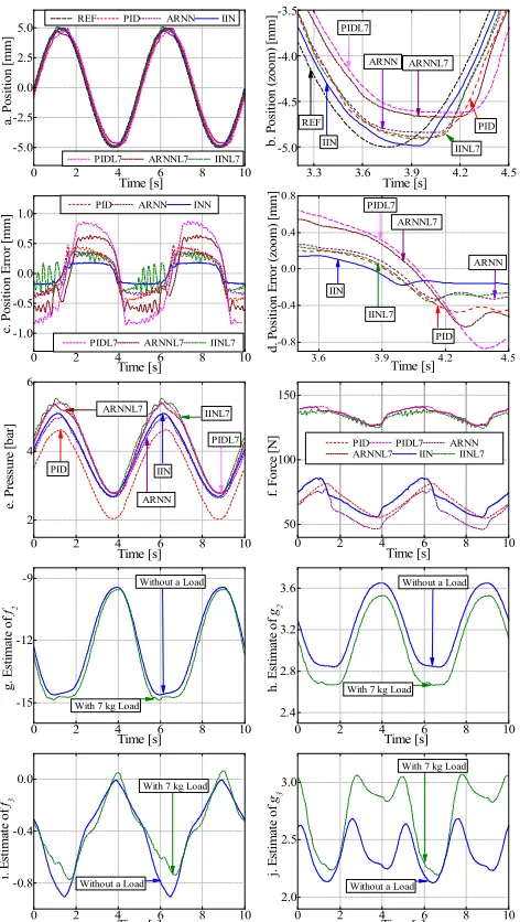
[image:10.595.54.289.562.736.2]with the 7 kg load, it was 0.65 mm (13%, ARNNL7 lines). Nevertheless, the best tracking performance was achieved by using the proposed controller, which integrated robustness and adaptability. It can be seen that due to the hard load, the force dynamics were decreased while the pressure dynamics were increased. The changes inside the system in the two load cases (free load and 7 kg load) were well represented using the proposed identification method. As a result, the proposed IIN controller could always keep the control error within an acceptable range where without a load, it was 0.18 mm (3.6%, IIN lines) and with the 7 kg load, it was 0.35 mm (7%, IINL7 lines).
Finally, Table III summarizes the root-mean-square (RMS) errors of the three compared controllers for all of the aforementioned case studies. As shown in the table, the proposed controller always obtained better results than the others under the same experimental conditions. These results demonstrate that the effectiveness and feasibility of the designed controller are proven.
0 2 4 6 8 10
-5.0 -2.5 0.0 2.5
5.0 REF PID ARNN IIN
PIDL7 ARNNL7 IINL7
Time [s]
a.
P
os
it
io
n
[m
m
]
3.3 3.6 3.9 4.2 4.5 -5.0
-4.5 -4.0 -3.5
Time [s]
b.
Po
si
ti
on
(z
oo
m
)
[m
m
]
REF PID
PIDL7
ARNN ARNNL7
IIN
IINL7
0 2 4 6 8 10
-1.0 -0.5 0.0 0.5
1.0 PID ARNN INN
PIDL7 ARNNL7 IINL7
c.
P
os
it
io
n
E
rr
or
[m
m
]
Time [s] 3.6 3.9 4.2 4.5
-0.8 -0.4 0.0 0.4 0.8
IINL7 IIN
PID ARNN ARNNL7 PIDL7
d.
Po
si
ti
on
E
rr
or
(z
oo
m
)
[m
m
]
Time [s]
0 2 4 6 8 10
2 4 6
ARNN IIN PID
ARNNL7 IINL7
PIDL7
e.
P
re
ss
ur
e
[b
ar
]
Time [s] 0 2 4 6 8 10
50 100 150
PID PIDL7 ARNN
ARNNL7 IIN IINL7
f.
Fo
rc
e
[N
]
Time [s]
0 2 4 6 8 10
-15 -12 -9
With 7 kg Load Without a Load
g.
E
st
im
at
e
of
f2
Time [s] 0 2 4 6 8 10
2.4 2.8 3.2 3.6
With 7 kg Load Without a Load
h.
E
st
im
at
e
of
g2
Time [s]
0 2 4 6 8 10
-0.8 -0.4 0.0
Without a Load With 7 kg Load
i.
E
st
im
at
e
of
f3
Time [s] 0 2 4 6 8 10
2.0 2.5 3.0
With 7 kg Load
Without a Load
j.
E
st
im
at
e
of
g3
[image:11.595.54.290.321.739.2]Time [s] Fig. 9. Experimental data with respect to case study 4.
TABLE III
PERFORMANCECOMPARISON OFALLSTUDIEDEXPERIMENTS
Case Trajectory RMS Error
PID ARNN IIN
Case 1 Sin 0.05Hz-10mm 0.691 0.235 0.200 Free-load
Case 2 Smooth multi-step 0.451 0.401 0.153 Free-load
Case 3 Sin 10mm
0.5 Hz 0.96 0.550 0.368 1Hz 1.926 1.142 0.439 Free-load 1.5Hz 3.554 2.495 0.756 Case 4-1
Sin 0.2Hz-5mm 0.339 0.291 0.156 Free-load
Case 4-2 Sin 0.2Hz-5mm
0.525 0.376 0.203 Loading Load 3kg
Case 4-3 Sin 0.2Hz-5mm 0.638 0.433 0.216 Loading Load 5kg
Case 4-4 Sin 0.2Hz-5mm 0.676 0.502 0.247 Loading Load 7kg
VI. CONCLUSION
In this study, an advanced control approach, “integrated intelligent nonlinear controller”, is developed and successfully applied to position tracking control of a PAM system. The IIN controller is constructed based on the new online estimation method and the robust nonlinear approach. The estimation method is employed to represent the system dynamics by neural networks in the state-space form while the robust control approach combines the sliding mode and backstepping techniques incorporating with the improvements to realize the control objective. The convergences of the model optimization and the closed-loop control system are theoretically ensured through Lyapunov stability conditions.
The PAM testing system was set up to investigate the position tracking task. Furthermore, typical PID and intelligent ARNN controllers were also implemented together with the IIN controller to control this system. The real-time control experimental results for the different cases of the references and load conditions confirmed the effectiveness and feasibility of the proposed approach in real-time applications.
However, there are some drawbacks that should be considered in future research. From Remark 2, we note that to improve the estimation result, the design of the used neural network should be based on an exact mathematic model of the system. The effectiveness of the proposed algorithm can be further increased by developing a method to automatically tune both the estimation and control gains. For better tracking performance in real-time control, the sampling time should be reduced [45]. Note also that the valve dynamics must be considered in this case.
REFERENCES
[1] T. Noritsugu and T. Tanaka, “Application of rubber artificial muscle manipulator as a rehabilitation robot,”IEEE/ASME Trans. Mechatronics, vol. 2, no. 4, pp. 259-267, 1997.
[3] P. K. Jamwal, S. Q. Xie, S. Hussain, and J. G. Parsons, “An adaptive wearable parallel robot for the treatment of ankle injuries,”IEEE/ASME
Trans. Mechatronics, vol. 19, no. 1, pp. 64-75, 2014.
[4] P. Beyl, M. V. Damme, R. V. Ham, B. Vanderborght, and D. Lefeber, “Pleated pneumatic artificial muscle-based actuator system as a torque source for compliant lower limb exoskeletons,” IEEE/ASME Trans.
Mechatronics, vol. 19, no. 3, pp. 1046-1056, 2014.
[5] X. Zhu, G. Tao, B. Yao, and J. Cao, “Adaptive robust posture control of parallel manipulator driven by pneumatic muscles with redundancy,”
IEEE/ASME Trans. Mechatronics, vol. 44, no. 9, pp. 2248-2257, 2008.
[6] C. Chou and B. Hannaford, “Measurement and modeling of McKibben pneumatic artificial muscles,”IEEE Trans. Robot. Autom, vol. 12, no. 1, pp. 90-102, 1996.
[7] B. Tondu and P. Lopez, “Modeling and control of McKibben artificial muscle robot actuators,”IEEE Control Syst. Mag., vol. 20, no. 2, pp. 15-38, 2000.
[8] E. G. Hocking and N. M. Wereley, “Analysis of nonlinear elastic behavior in miniature pneumatic artificial muscles,” Smart Materials and
Structures, vol. 22, no. 1, pp. 1-14, 2013.
[9] C. Kothera, M. Jangid, J. Sirohi, and N. Wereley, “Experimental characterization and static modeling of McKibben actuators,” J. of
Mechanical Design, vol. 131, no. 9, pp. 1-10, 2009.
[10] P. A. Aron, M. Anjel, A. Javier, P. Ramon, and L. Joseba, “Modelling in Modelica and position control of a 1-DoF set-up powered by pneumatic muscles,”Mechatronics, vol. 20, no. 5, pp. 535-552, 2010.
[11] C. W. Kanchana and L. Thananchai, “Empirical modeling of dynamic behaviors of pneumatic artificial muscle actuators,”ISA Transactions, vol. 52, no. 6, pp. 825-834, 2013.
[12] T. V. Minh, T. Tjahjowidodo, H. Ramon, and H. V. Brussel, “A new approach to modeling hysteresis in a pneumatic artificial muscle using the Maxwell-slip model, “IEEE/ASME Trans. Mechatronics, vol. 16, no. 1, pp. 177-186, 2011.
[13] HPH. Anh and K. K. Ahn, “Identification of pneumatic artificial muscle manipulators by a MGA-based nonlinear NARX fuzzy model,”
Mechatronics, vol. 19, no. 1, pp. 106-133, 2009.
[14] HPH. Anh and K. K. Ahn, “Hybrid control of a pneumatic artificial muscle (PAM) robot arm using an inverse NARX fuzzy model,”Eng.
App. Artificial Intelligence, vol. 24, no. 4, pp. 697-716, 2011.
[15] K. Kawashima, T. Sasaki, A. Ohkubo, T. Miyata, and T. Kagawa, “Application of robot arm using fiber knitted type pneumatic artificial rubber muscles,” InProc. IEEE Int. Conf. Robotics and Automation, New Orleans, LA, 2004, pp. 4937-4942.
[16] S. Ganguly, A. Garg, A. Pasricha, and S. K. Dwivedy, “Control of pneumatic artificial muscle system through experimental modeling,”
Mechatronics, vol. 22, no. 8, pp. 1135-1147, 2012.
[17] J. H. Lilly, “Adaptive tracking for pneumatic muscle actuators in Bicep and Tricep configurations,“IEEE Trans. Neural Syst. Rehabil. Eng., vol. 11, no. 3, pp. 333-339, 2003.
[18] H. Aschemann and D. Schindele, “Sliding-mode control of a high-speed linear axis driven by pneumatic muscle actuators,” IEEE Trans. Ind.
Electron., vol. 55, no. 11, pp. 3855-3864, 2008.
[19] B. Tondu, K. Braikia, M. Chettouh, and S. Ippolito, “Second order sliding mode control for an anthropomorphic robot-arm driven with pneumatic artificial muscles,” In IEEE-RAS Int. Conf. Humanoid Robot, Paris, France, 2009, pp. 47-54.
[20] Y. Shtessel, M. Taleb, and F. Plestan, “A novel adaptive-gain supertwisting sliding mode controller: Methodology and application,”
Automica, vol. 48, no. 5, pp. 759-769, 2012.
[21] T. J. Jeh, M. J. Wu, T. J. Lu, F. K. Wu, and C. R. Huang, “Control of McKibben pneumatic muscles for a power-assist, lower-limb orthosis,”
Mechatronics, vol. 20, no. 6, pp. 686-697, 2010.
[22] M. K. Chang, J. J. Liou, and M. L. Chen, “T-S fuzzy model-based tracking control of a one-dimensional manipulator actuated by pneumatic artificial muscles,”Control Engineering Practice, vol. 19, no. 12, pp. 1442-1449, 2011.
[23] A. Hildebrandt, A. Sawodny, R. Neumann, and A. Hartmann, “A cascaded tracking control concept for pneumatic muscle actuators,”2003
European Control Conference, Cambridge, UK, 2003, pp. 2517-2522.
[24] X. Shen, “Nonlinear model-based control of pneumatic artificial muscle servo systems,”Control Engineering Practice, vol. 18, no. 3, pp. 311-317, 2010.
[25] B. Taheri, D. Case, and E. Richer, “Adaptive suppression of severe pathological tremor by torque estimation method,”IEEE/ASME Trans.
Mechatronics, vol. 20, no. 2, pp. 717-727, 2015.
[26] D. G. Caldwell, G. A. Medrano-Cerda, and M. Goodwin, “Control of pneumatic muscle actuators,”IEEE Control Syst., vol. 15, no. 1, pp. 40-48, 1995.
[27] X. Zhu, G. Tao, B. Yao, and J. Cao, “Integrated direct/indirect adaptive robust posture trajectory tracking control of a parallel manipulator driven by pneumatic muscles,”IEEE Trans. Control Syst. Technol., vol. 17, no. 3, pp. 576-588, 2009.
[28] T. Hesselroth, K. Sarkar, P. Patrick van der Smagt, and K. Schulten, “Neuron network control of a pneumatic robot arm,”IEEE Trans. Syst.,
Man, Cybern., vol. 24, no. 1, pp. 28-38, 1994.
[29] K. K. Ahn and HPH. Anh, “Design and implementation of an adaptive recurrent neural networks (ARNN) controller of the pneumatic artificial muscle (PAM) manipulator,”Mechatronics, vol. 19, no. 6, pp. 816-828, 2009.
[30] K. Xing, Y. Wang, Q. Zhu, and H. Zhou, “Modeling and control of Mckibben artificial muscle enhanced with echo state networks,”Control
Engineering Practice, vol. 20, no. 5, pp. 477-488, 2012.
[31] S. W. Chan, J. H. Lilly, D. W. Repperger, and J. E. Berlin, “Fuzzy PD+I learning control for a pneumatic muscle,” InThe IEEE Int. Conf. Fuzzy
Systems, 2003; 278-283.
[32] TDC. Thanh and K. K. Ahn, “Nonlinear PID control to improve the control performance of 2 axes pneumatic artificial muscle manipulator using neural network,”Mechatronics, vol. 16, no. 9, pp. 577-587, 2006. [33] HPH. Anh, “Online tuning gain scheduling MIMO neural PID control of
the 2-axes pneumatic artificial muscle (PAM) robot arm,”Expert Systems
with Applications, vol. 37, no. 9, pp. 6547-6560, 2010.
[34] G.Andrikopoulos, G. Nikolakopoulos, and S. Manesis, “Advanced nonlinear PID-Based antagonistic control for pneumatic muscle actuators,”IEEE Trans. Ind. Electron, vol. 61, no. 12, pp. 6929-6937, 2014.
[35] L. D. Khoa, D. Q. Truong, and K. K. Ahn, “Synchronization controller for a 3-R planar parallel pneumatic artificial muscle (PAM) robot using modified ANFIS algorithm,”Mechatronics, vol. 23, no. 4, pp. 462-479, 2013.
[36] H. Jahanabadi, M. Mailah, M. Z. M. Zain, and H. M. Hooi, “Active force with fuzzy logic control of a two-link arm driven by pneumatic artificial muscles,”Journal of Bionic Engineering, vol. 8, no. 4, pp. 474-484, 2011. [37] S. Q. Xie and P. K. Jamwal, “An iterative fuzzy controller for pneumatic muscle driven rehabilitation robot,” Expert Systems with Applications, vol. 38, no. 7, pp. 8128-8137, 2011.
[38] M. Chandrapal, X. Chen, W. Wang, and C. Hann, “Nonparametric control algorithms for a pneumatic artificial muscle,” Expert Systems with
Applications, vol. 39, no. 10, pp. 8636-8644, 2012.
[39] G. Andrikopoulos, G. Nikolakopoulos, and S. Manesis, “Pneumatic artificial muscles: A switching model predictive control approach,”
Control Engineering Practice, vol. 21, no. 12, pp. 1653-1664, 2013.
[40] B. Iranpanah, M. Chen, A. Patriciu, and S. Sirouspour, “A pneumatically actuated target stabilization device for MRI-guided breast biopsy,”
IEEE/ASME Trans. Mechatronics, vol. 20, no. 3, pp. 1288-1300, 2015
[41] Proportional directional control valves MPYE, Festo Company (2015). [Online]. Available: https://www.festo.com/cat/en-gb_gb/data/doc_ENGB/PDF/EN/MPYE_EN.PDF.
[42] J. L. Castro, “Fuzzy logic controllers are universal approximators,”IEEE
Trans. Syst. Man, and Cybern., vol. 25, no. 4, pp. 629-635, 1995.
[43] B. Yao, F. Bu, J. Reedy and G. T. C. Chiu, “Adaptive robust motion control of single-rod hydraulic actuators: Theory and Experiments,”
IEEE/ASME Trans. Mechatronics, vol. 5, no. 1, pp. 79-91, 2000.
[44] S. Hodgson, M. Tavakoli, M. T. Pham, and A. Leleve, “Nonlinear discontinuous dynamics averaging and PWM-based sliding control of solenoid-valve pneumatic actuators,”IEEE Trans. Mechatronics, vol. 20, no. 2, pp. 876-888, 2015.
Dang Xuan Bareceived the B.S and M.S. degrees from Ho Chi Minh City University of Technology in 2008 and 2012, respectively, both in Automatic Control Engineering. He is currently earning a Ph.D degree at the University of Ulsan. His research interests include intelligent control, nonlinear control, modern control theories and their applications.
Truong Quang Dinh received the B.S. degree in mechanical engineering from Ho Chi Minh City University of Technology in 2001, and the Ph.D. degree in mechanical engineering from the University of Ulsan, Ulsan, Korea, in 2010. Currently, he is a Researcher at WMG, University of Warwick. His research interests focus on control theories and applications, fluid power control systems, energy saving and power management systems, low carbon technologies for transports and construction sectors, and smart sensors and actuators.