ISSN: 1816-9503
© Medwell Journals, 2009
Corresponding Author: M.C. Ndinechi, Department of Electrical and Electronic Engineering, Federal University of Technology,
Algorithm for Applying Decimator Structures in Digital Signal Processing
Systems for Energy Conservation
M.C. Ndinechi, N. Onwuchekwa and G.A. Chukwudebe Department of Electrical and Electronic Engineering,
Federal University of Technology, Owerri, Nigeria
Abstract: Digital Signal Processing (DSP) has become one of the most powerful technologies in reshaping science and engineering especially in the areas of communication and medicine. In this research, DSP applications, where the signal at a given sampling rate needs to be converted into another signal with a different sampling rate known as multirate systems are investigated. This multirate DSP has been found useful in such application like digital audio, video and even GSM technology. The design of digital filters and multirate system using decimator structures is presented. The research is implemented using MATLAB software. Several plotsTM
obtained showed that decimator structures reduce the number of operations required for a particular application. With the sampling rate reduced, the processor runs at a lower clock rate thereby producing less heat. This will eventually lead to lower power/battery consumption.
Key words: Digital, signal, energy, conservation, decimator, multirate, MATLABTM
INTRODUCTION functions in a transformed domain. Likewise, the Digital Signal Processing (DSP) has become one of original domain of the signal or in a transformed domain. the most powerful tools in reshaping science and A digital signal processor is an integrated engineering. Revolutionary changes have already been circuit designed for high-speed data manipulations made in a broad range of fields in communications, (Peterson et al., 2000). The DSP performs multiplication medicine, radar and sonar, hi-fi music reproduction and oil in a single cycle by implementing all shifts and add prospecting using DSP systems. So, it appeals to the operations in parallel. When general purpose DSPs are engineer, the medical doctor as well as the musician. not fast enough, the signal is either processed using Under suitable software environment, DSP allows analogue circuits which may have some drawbacks, or experimentation with sounds, images and video which application specific DSP hardware. Digital signal contain a number of well defined mathematical problems, processing by its nature requires many manipulations of from filtering to multirate to sigma delta modulation and to the form A = B×C + D. This may appear to be simple but error correction, using Fast Fourier Transforms (FFT), when speed is also required, only dedicated hardware can digital filters and multirate filters as building blocks perform this task. Digital signal processors have
(Cristi, 2004). specialized instruction that allows them to multiply, add
A signal can be generated synthetically or by and save the result in a single instruction cycle. This computer simulation to carry information. The objective of instruction is usually called MAC (Multiply and signal processing is to extract useful information carried Accumulate) (Peterson et al., 2000).
( )
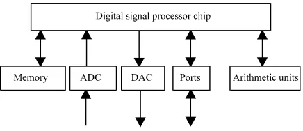
[image:2.612.78.296.97.191.2]y m x(mM )= Fig. 1: Typical contents of a DSP hardware
Compact Disc (CD) or when mixing signals with different standards. Some other reasons for resampling may be when there is need to pass data between two systems that use incompatible sampling rates. In the bid to solve this problem, multirate digital signal processing was developed (Crochiere and Rabiner, 1983). Therefore, the objective of this research is to investigate the problems associated with changing of sampling frequency of a discrete signal since it can lead to loss of valuable information or distortion. With this, the number of operations is highly reduced as well as heat dissipation thereby conserving energy.
Advantages and disadvantages of DSP: Analogue signal processing involves linear operations such as amplification, filtering, integration and differentiation and non-linear operations such as squaring, rectification etc. Some of the limitations of analogue signal processing are restricted accuracy and dynamic range, limited speed of operation, component drift and sensitivity to noise. On the other hand, digital signal processing involves numerical operations such as addition, multiplication, data transfer and logical operations. Consequently, digital signal processing offers some clear advantages over analogue signal processing. These include:
Programmability: A single piece of digital DSP hardware can perform many functions.
Upgradeability: Once a design have been implemented, one may want to upgrade or add new functions or adapt to a new environment altogether.
Flexibility: A single DSP board can be made to perform many functions by simply loading new programs into it. This flexibility reduces design time and complexity. Stability: DSP gives stable performance over time. Temperature effect: A temperature sensitive analogue circuit will definitely perform quite differently in different
Fig. 2: Block diagram of discrete-time digital processing of a continuous time signal
climatic regions of the world. Digital circuits do not change their characteristics with temperature. They either work or do not work.
Digital repeatability: A properly designed digital circuit will reproduce the same result every time in addition to being identical from unit to unit.
Digital signal processing equally have some disadvantages. One of such disadvantages is increased system complexity in the digital processing of analogue signals (Mitra, 2006). Another disadvantage is the limited range of frequencies available for processing.
Fundamental of Digital Signal Processing (DSP): DSP is achieved by sampling the analogue signal at regular intervals and converting each of these samples, with a binary number quantization. Several operations such as filtering, resampling etc can then be performed on the sequence of numbers (signal). The basic building block of the discrete-time digital processing of a continuous time signal is as shown in Fig. 2 where, x (t) and y (t) are analogue signals, while x(n) and y(n) are discrete time signals. The DSP processor implements the desired algorithm.
MATERIALS AND METHODS
Multirate signal processing: The process of converting the given rate of a signal into a different rate is called sampling rate conversion. Systems that employ multiple sampling rates in the processing of digital signals are called multirate digital processing systems (http://www.dspguru.org/Info/faqs/multirate/decim.htm; http://www.idealgroup.com/downloads/excerpts/190307 08300Book.Ex.Pdf:). The reduction of a sampling rate is called decimation because the original sample set is reduced or decimated (http://www.dspguru.org/Info/faqs/ multirate/basics.htm).
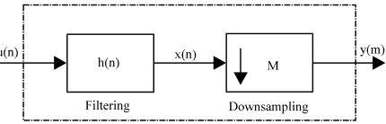
Decimation consists of two stages; filtering and downsampling as shown in Fig. 3. Downsampling reduces the input sampling rate f by an integer factor M. The1
output signal y(m) is called a downsampled signal and is obtained by taking only every Mth sample of the input signal and discarding all others:
( )
'
M
x n x (n)C (n)=
1 for n mM M 0 otherwise
C (n)=
{
=n j2 k M 1 M M k 0 1
C (n) C(k)e M π − = =
∑
n j2 k M 1 M M n 0C (K) C (n)e − π − = =
∑
n j2 k M 1 M M k 0 1C (n) e
M π −
=
=
∑
' j ' j n
n
j n M n
x (e ) x (n)e
x(n)C (n)e ∞
ω − ω
=−∞ ∞ − ω =−∞ = =
∑
∑
n j2 K M 1' j M j n
n k 0
1
x (e ) x(n) e e M
π
∞ −
ω − ω
=−∞ =
=
∑
∑
n
2 k
M 1 )
' j jn ( M
k 0 n
x (e ) x(n)e π − ∞
ω − ω−
= =−∞
=
∑ ∑
' j j n
n
x (e ) x(n)e ∞
ω − ω
=−∞
=
∑
2 k 2 k
M M
j( ) jn( )
n
x(e π ) x(n)e π ∞
ω− − ω−
=−∞ =
∑
2 k M M 1 j( ) ' j k 0 1x (e ) xe
M π − ω− ω = =
∑
M M j jn ' ' nx (eω ) x (n)e ω ∞
−
=−∞
=
∑
M M
j j( )mM
' '
n
j m n
x (e ) x (mM)e x(mM)e
ω ∞ − ω
[image:3.612.76.291.99.168.2]=−∞ ∞ − ω =∞ = =
∑
∑
Fig. 3: Decimator stages
To model the downsampling process, it is convenient to divide it into two steps. The output of the first step is the signal x (n), which is obtained by setting all samples’
whose indices are not integer multiples of M to zero. In the second step, all zeroes that were introduced in the first step are discarded. This result is the downsampled signal. The downsampling operation is not invertible because it requires setting some of the samples to zero i.e., x(n) cannot be recovered from y(m) exactly but can only compute an approximate value.
The sampling rate is not altered during the first step so that the signals x(n) and x (n) have the same sampling’
rate. The signal x (n) can be considered as a multiplication’
of x(n) with the discrete sampling function C (n) where,M
M denotes the downsampling factor.
(2) Where:
and
m = , , 1, 0, +1, , ,
-The sampling function C (n) is periodic with periodM
M and as such can be represented by the Fourier series expansion:
(3)
where, C (k) are complex value Fourier series coefficients defined by:
(4)
Substituting Eq. 4 into 3, it follows that C (k) = 1 for all K. Hence,
(5)
to analyze the frequency representation of first step of down sampling, Fourier Transform (FT) of the sequence x (n) is computed using Eq. 2.’
(6)
Using the relationship established in Eq. 5 and 6 becomes:
(7)
By interchanging the sums in Eq. 7, x (e ) becomes:’ jT
(8)
Computing the FT of x(n)
(9)
Applying the frequency shift property of FT gives: (10)
The expression on the right hand side of Eq. 10 resembles the one in Eq. 8. Then, it can be concluded that: (11)
From Eq. 11, it will be observed that the amplitude is scaled by 1/M and that the replicas of the input spectrum are introduced at multiples of 2B/M. The zeros previously introduced have to be eliminated. This operation does not change the content of the signal x (n), rather it just'
introduces time scaling by a factor of 1/M. Because the operations in time and frequency are inverse to each other, the frequency scale will be multiplied by M i.e., x (e' jT/M) becomes y(e ).jT
Again, using the definition of FT for x (n)'
(12)
Because x (n) is non zero for only n = mM, then '
M
j
' j m j
n
x (eω ) y(m)e y(e ) ∞
− ω ω
=−∞
=
∑
=2 k M
M 1
j( )
jM ' j
K 0
1
y(e ) x (e ) x(e )
M
π
− ω−
ω ω
=
= =
∑
n
n
x(z) x(n)z ∞
−
=−∞
=
∑
j
j z e
x (z) ω x(e ) ω = =
M 1 2 k
j
M ' M
K 0
1
y(z ) x (z) x(ze )
M
− − π
=
= =
∑
Substituting Eq. 1 into 13 and using the definition of Consequently, the expression in Eq. 15 can be
F.T. for y(m). expressed in terms of z-transform as:
(14) (18)
Using Eq. 11 and 14 can be rewritten as: RESULTS AND DISCUSSION
(15)
Equation 15 gives the expression for the downsampled signal. Sometimes, it is more convenient to express the downsampled signal in terms of its z-transform. For a sequence x(n), its z-transform is defined as:
(16)
where, z is a complex variable given by z = re . It is welljT
known that when it exists, the F.T. is simply x(z) with z =e .jT
(17)
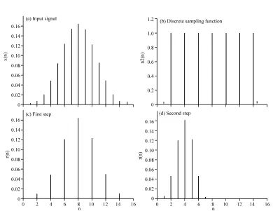
To illustrate downsampling in the time domain, consider the input signal shown in the Fig. 4a with the down sampling factor of M = 2. The corresponding sampling function for n = 0, 2…, 16 is given in Fig. 4b. Figure 4c demonstrates the first step of down sampling, where every second sample is set to zero. In the second step, Fig. 4d, the zeros introduced in the previous step are eliminated to finally obtain the down sampled signal. It can be observed that the downsampled signal is a compressed in time version of the input signal.
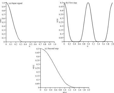
[image:4.612.105.495.401.702.2]The frequency domain representation of the downsampling is as shown in Fig. 5a during the first step, Fig. 5b, one image (M-1 = 1) is introduced in the interval (0, 2B) and the amplitude of the spectrum is scaled by ½. In the second step, Fig. 5c, the frequency is scaled by m = 2, as proved in Eq. 15.
M M
1, j
0,
H(e )
ω
π
ω ≤ ω
≤ ω ≤π
[image:5.612.106.481.94.399.2] =
Fig. 5: Downsampling in frequency domain
It can be observed that the spectrum of the Downsampling operation in the time and frequency downsampled signal is the input spectrum stretched by
2, while in the time domain, the opposite was true (compressed by a factor of 2) because the time and frequency representations are inverse to each other. Aliasing effect: The individual spectra obtained during the first step of downsampling are the repeated replicas of the original spectrum. If the original signal is not band limited to B/M, the replicas will overlap. This overlapping effect is called aliasing. In order to avoid aliasing, it is necessary to limit the spectrum of the signal before downsampling to below B/M by allowing low pass filtering to precede the downsampler (Lyons) as shown in Fig. 3.
This filter is called a decimation or anti-aliasing filter. The exact filter specifications depend on how much aliasing (if any) is permitted. The specifications for the low pass decimation filter are given by as (http://www.ifn. et-tudresden.de/MNS/veroeffertlichugen/2000/Hentsche. com):
(19)
domain using MATLAB :TM We investigated the downsampling of a sinusoidal input sequence using MATLAB (Chapman, 2002).
The codes for the program are listed in Appendix 1. Its input data are the length of the input sequence, the downsampling factor and the frequency of the sinusoid in Hz. It then plots the input and its downsampled version. The result obtained for a length of 50 sinusoidal sequences with a frequency of 0.042 H andZ
with a downsampling factor of 3 is as shown in Fig. 6. From these plots, it can be verified that the relation between the output and the input sequences satisfied Eq. 1.
We further investigated the frequency domain properties of the downsampling using MATLABTM .
Fig. 6: Input and output plots generated by running appendix 1
Fig. 7: Input and output plots generated by running appendix 2
Fig. 8: Input and output plots generated by running appendix 3
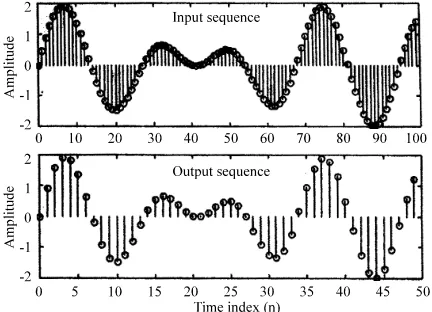
Decimation operation using MATLAB: We further carried out the decimation of a sum of two sinusoidal
sequences of normalized frequencies f and f by an1 2
arbitrary down sampling factor M using the MATLABTM
codes listed in Appendix 3. The input data to the program are the length (N) of the input x(n), the downsampling factor M and the two normalized frequencies in Hz. The program uses a Finite Impulse Response (FIR) low-pass decimation filter with stop band edge at B/M so as to satisfy Eq. 19. The input and output sequences are as indicated in Fig. 8. For N = 100, M = 2, F = 0.043 and1
F = 0.031.2
CONCLUSION
The sampling rate conversion (Mutirate) can be viewed as another way of filter design. It must satisfy all the specification necessary to avoid signal degradation such as aliasing and imaging while keeping the number of coefficients at minimum to further reduce computational cost. Multirate Digital Signal Processing (MDSP) has proved to be a powerful method of significantly reducing the number of computation in the sampling rate conversion processes. This is certainly an important issue, especially in telecommunications. Of particular importance is in GSM (Global System for Mobile) applications. With the sampling rate reduced, the processor runs at a lower clock rate thereby producing less heat. This will eventually lead to lower power/battery consumption. Users will have to use their devices longer without the need to recharge more regularly.
APPENDIX 1
% Illustration of Down-sampling by an Integer factor %
clf; n = 0: 49; m= 0:50*3-1; x = sin(2*pi*0.042*m); y = x([l:3:length(x)]); subplot(2,l,l)
Stem(n,x(l:50)); axis([0 50 -1.2 1.2]); title('Input Sequence');
xlabel(Time index n'); ylabel('Amplitude'); subplot(2,l,2)
stem(n, y); axis([0 50-1.2 1.2]); tille('Output Sequence'); xlabel(‘Time index n'); ylabel('Amplitude');
From these plots it can be verified that the relation between the output and input sequences satisfies Eq. 3.1
APPENDIX 2
Effect of Down-sampling in the frequency domain Use fir2 to create a band-limited input sequence clf;
freq = [0 0.42 0.48 1]; mag = [0 1 0 0]; x=fir2(101, freq, mag);
Evaluate and plot the input spectrum [Xz,w]==freqz(x, 1,512); subplot(2,l,l)
[image:6.612.75.291.502.658.2]xlabel('\omega/\pi'); ylabel('Magnitude'); title('Input Spectrum');
Generate the up-sampled sequence
M = input('Type in the Down-sampling factor = '); Type in the Down-sampling factor = 2
Y = x([l:M:lengthCx)]);
% Evaluate and plot the output spectrum [Yz, w] = freqz(y, 1, 512);
subplot(2,1,2); plot(w/pi, abs(Yz); grid
xlabel(‘\omega/\pi’); ylabel(‘Magnitude’); title(‘Output Spectrum’);
APPENDIX 3
% Program 4.5
% Illustration of Decimation process clf;
M = input('Down-sampling factor = '); Down-sampling factor == 2 n=0:99;
x= sin(2*pi*0.043*n) + sin(2*pi*0.031*n); y = decimate(x,M,'fir');
subplot(2,l,l); stem(n,x(l:100)); title(‘Input Sequencer’);
xlabel('Time index n');ylabel('Amplitude'); subplot(2,l,2);
m=0:(100/M)-l; stem(m,y(l:100/M)); title('Output Sequence'); xlabel('Time index n'); ylabel('Amplitude')
REFERENCES
Cristi, R., 2004. Modern digital signal processing. Brooks/Cole, pp: 1-10, 234-264. http://www.amazon. com/Modern-Digital-SignalProcessing-Roberto/dp/ 0534400957.
Chapman, S.J., 2002. MATLAB Programming for Engineers. 2nd Edn. Bookware Companion Series, Brooks/Cole. ISBN: 0-534-39056-0.
Crochiere, R.E. and L.R. Rabiner, 1983. Multirate digital signal processing. Prentice Hall. Englewood Cliffs, N.J.
Eyre, J., 2001. The digital signal processor derby. IEE Spectrum, 38 (6): 62-68. http://www.research.ibm. com/journal/rd/472/morenref-html.
Mitra, S.K., 2006. Digital Signal Processing: A computer Based Approach. 3rd Edn. Mc Graw-Hill. http://www. ucd.ie/math-phy/courses/SigPro/Lecture1.pdf. Peterson, C., R. Sikora, M.B. Akhan, I. Munro and