Efficient learning methods to tune algorithm parameters

(1)

University of Warwick institutional repository:

http://go.warwick.ac.uk/wrap

A Thesis Submitted for the Degree of PhD at the University of Warwick

http://go.warwick.ac.uk/wrap/58890

This thesis is made available online and is protected by original copyright.

Please scroll down to view the document itself.

(2)

Library Declaration and Deposit Agreement

1. STUDENT DETAILS Please complete the following:

Full name: ………. University ID number: ………

2. THESIS DEPOSIT

2.1 I understand that under my registration at the University, I am required to deposit my thesis with the University in BOTH hard copy and in digital format. The digital version should normally be saved as a single pdf file.

2.2 The hard copy will be housed in the University Library. The digital version will be deposited in the University’s Institutional Repository (WRAP). Unless otherwise indicated (see 2.3 below) this will be made openly accessible on the Internet and will be supplied to the British Library to be made available online via its Electronic Theses Online Service (EThOS) service.

[At present, theses submitted for a Master’s degree by Research (MA, MSc, LLM, MS or MMedSci) are not being deposited in WRAP and not being made available via EthOS. This may change in future.]

2.3 In exceptional circumstances, the Chair of the Board of Graduate Studies may grant permission for an embargo to be placed on public access to the hard copy thesis for a limited period. It is also possible to apply separately for an embargo on the digital version. (Further information is available in the Guide to Examinations for Higher Degrees by Research.)

2.4 If you are depositing a thesis for a Master’s degree by Research, please complete section (a) below. For all other research degrees, please complete both sections (a) and (b) below:

(a) Hard Copy

I hereby deposit a hard copy of my thesis in the University Library to be made publicly available to readers (please delete as appropriate) EITHER immediately OR after an embargo period of ………... months/years as agreed by the Chair of the Board of Graduate Studies.

I agree that my thesis may be photocopied. YES / NO (Please delete as appropriate)

(b) Digital Copy

I hereby deposit a digital copy of my thesis to be held in WRAP and made available via EThOS.

Please choose one of the following options:

EITHER My thesis can be made publicly available online. YES / NO(Please delete as appropriate)

OR My thesis can be made publicly available only after…..[date] (Please give date)

YES / NO(Please delete as appropriate)

OR My full thesis cannot be made publicly available online but I am submitting a separately identified additional, abridged version that can be made available online.

YES / NO (Please delete as appropriate)

(3)

Whether I deposit my Work personally or through an assistant or other agent, I agree to the following:

Rights granted to the University of Warwick and the British Library and the user of the thesis through this agreement are non-exclusive. I retain all rights in the thesis in its present version or future versions. I agree that the institutional repository administrators and the British Library or their agents may, without changing content, digitise and migrate the thesis to any medium or format for the purpose of future preservation and accessibility.

4. DECLARATIONS (a) I DECLARE THAT:

I am the author and owner of the copyright in the thesis and/or I have the authority of the authors and owners of the copyright in the thesis to make this agreement. Reproduction of any part of this thesis for teaching or in academic or other forms of publication is subject to the normal limitations on the use of copyrighted materials and to the proper and full acknowledgement of its source.

The digital version of the thesis I am supplying is the same version as the final, hard-bound copy submitted in completion of my degree, once any minor corrections have been completed.

I have exercised reasonable care to ensure that the thesis is original, and does not to the best of my knowledge break any UK law or other Intellectual Property Right, or contain any confidential material.

I understand that, through the medium of the Internet, files will be available to automated agents, and may be searched and copied by, for example, text mining and plagiarism detection software.

(b) IF I HAVE AGREED (in Section 2 above) TO MAKE MY THESIS PUBLICLY AVAILABLE DIGITALLY, I ALSO DECLARE THAT:

I grant the University of Warwick and the British Library a licence to make available on the Internet the thesis in digitised format through the Institutional Repository and through the British Library via the EThOS service.

If my thesis does include any substantial subsidiary material owned by third-party copyright holders, I have sought and obtained permission to include it in any version of my thesis available in digital format and that this permission encompasses the rights that I have granted to the University of Warwick and to the British Library.

5. LEGAL INFRINGEMENTS

I understand that neither the University of Warwick nor the British Library have any obligation to take legal action on behalf of myself, or other rights holders, in the event of infringement of intellectual property rights, breach of contract or of any other right, in the thesis.

Please sign this agreement and return it to the Graduate School Office when you submit your thesis.

(4)

by

Jawad A. El-Omari

Supervised by Professor Juergen Branke

A thesis submitted in the partial fulfilment of the requirements

for the degree of Doctor of Philosophy in

Operational Research and Management Sciences

(5)

Acknowledgement vii

List of figures viii

List of tables xiv

Declaration xix

Abstract xx

List of abbreviations xxi

Chapter 1: Introduction

1.1. Motivation and problem statement………. 1

1.2. Solution approaches………. 2

1.3. Contributions………. 6

1.3.1. Meta-Optimization with a Flexible Budget………... 6

1.3.2. Racing with a self-adaptive significance level………. 8

1.3.3. One-way Racing with an intelligent budget allocation……… 9

1.4. Organization of the thesis………... 10

Chapter 2: Literture Review 2.1 Introduction……….. 11

2.2 Classification……… 11

2.3 Online control……….. 14

2.3.1 Single step look-ahead………. 14

2.3.2 Multi-step look-ahead……….. 19

2.4 Offline tuning……….. 23

2.4.1 Model-free methods……….. 23

2.4.1.1 Meta-optimization………. 23

2.4.1.2 Computational budget allocators………... 28

2.4.2 Model Based Methods……….. 35

2.5 Online or offline?... 39

2.6 Prospect research………... 41

(6)

3.1 Introduction……….. 44

3.2 Meta-optimization……… 44

3.2.1 Meta-optimization with a fixed budget……….. 45

3.2.2 Meta-optimization with a flexible budget (first contribution)…… 46

3.3 Budget allocators………. 50

3.3.1 OCBA maximizing the probability of correct selection………….. 51

3.3.2 CBA………. 53

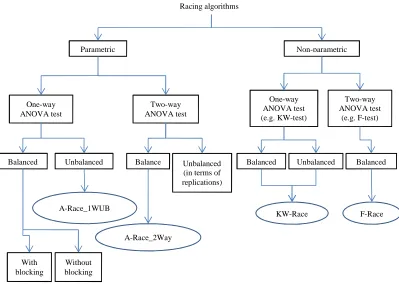
3.4 Racing algorithms……… 55

3.4.1 Parametric Racing………. 56

3.4.1.1 A background on normal-model based ANOVA………... 57

3.4.1.2 Violating normal-model based ANOVA assumptions……….. 63

3.4.1.3 Applicability of ANOVA models to Racing algorithms…….. 66

3.4.2 Non-parametric Racing………. 67

3.4.2.1 F-Race………. 67

3.4.2.2 KW-Race………. 70

3.5 Racing with reset (second contribution)……….. 73

3.6 One-way Racing with intelligent budget allocation (third contribution) 76 3.7 Conclusion……… 77

Chapter 4: Experiments, Results, and Analysis Meta-Optimization with a Flexible Budget 4.1 Introduction………. 78

4.2 Experimental setup………. 78

4.2.1 Competing algorithms and performance measures………. 78

4.2.2 Training and testing sets……… 81

4.3 Results………. 82

4.3.1 Results for Set-1……….. 82

4.3.2 Results for Set-2……….. 87

4.3.3 Results for Set-3……….. 94

4.3.4 Time savings……… 100

4.3.5 Summary……….. 100

4.4 Conclusion……….. 101

Chapter 5: Experiments, Results, and Analysis Computational Budget Allocators 5.1 Introduction……… 103

5.2 Experimental setup……… 103

(7)

5.3.1.1 Case 1: Monotonically increasing means with

equal variances....……….……… 108 5.3.1.2 Case 2: Monotonically increasing means with

exponentially decreasing variances……… 117 5.3.1.3 Case 3: Monotonically increasing means with

exponentially increasing variances………. 124 5.3.1.4 Case 4: Means and variances are randomly selected……… 130

5.3.1.5 Summary……….. 137

5.3.2 Results for Set-2……….. 138

5.3.2.1 Case 1 and Case 4: Monotonically increasing means with equal variances, and means and variances are randomly

selected……… 140

5.3.2.2 Case 2 and Case 3: Monotonically increasing means with

increasing or decreasing variance……….. 142

5.3.2.3 Summary……….. 145

5.3.3 Results for Set-3……….. 146

5.3.3.1Case 1: Monotonically increasing means with

equal variances……….………. 147 5.3.3.2 Case 2: Monotonically increasing means with

linearly decreasing variances……….. 154 5.3.3.3 Case 3: Monotonically increasing means with

linearly increasing variances……….…. 159 5.3.3.4 Case 4: Means and variances are randomly selected…………. 166

5.3.2.4 Summary……… 172

5.4 Conclusion……….. 173

Chapter 6: Conclusion

6.1. Summary of contributions………. 175

6.1.1.Meta-Optimization with a Flexible Budget……… 175 6.1.2. Racing with a self-adaptive significance level and

one-way Racing with an intelligent budget allocation………… 177 6.2. Limitations, extensions, and future research……….. 180

References

Reference list………..………. 182

Appendix

A1. CBA vs. OCBA……… 198

A2. A-Race_2Way setting the budget………. 201

(8)

(9)

Chapter 1: Introduction

No. Description Page

1.1 Effect of different parameter settings on an algorithm’s performance on a_{minimization problem} 1

1.2 _{For a minimization problem, a greedy parameter is suitable for small budgets,}Different parameter settings are suitable for different budgets. but not larger ones

3

1.3 Configuring parameters with a higher level algorithm 4

1.4 The performance of an algorithm, minimization problem, under three different parameter settings, each is suitable for a different computational budget.

7

Chapter 2: Literature Review

2.1 The proposed categorization of algorithm configurators 13

2.2 Meta-optimization framework 24

2.3

An example of allocating a budget between five parameter settings withn0= 5. The numbers indicate the iteration in which the runs were made. For instance,

parameter settings 1 and 3 were run in the second iteration with parameter setting 1 being tested on instances 6-9, while parameter settings 3 was run on

instance 6

29

Chapter 3: Theory and Methodology

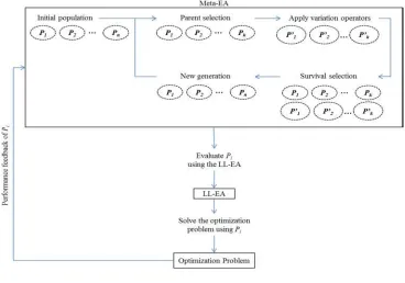
3.1 A sample meta-EA 45

3.2 Convergence curves of an algorithm, applied to a minimization problem, under

two different parameter settings 46

3.3 Ranking parameter settings using the Flexible Budget method. Assume a

minimization problem 48

3.4 Area Under the Curve as a secondary criterion for the Flexible-Budget method.

Assume a minimization problem 48

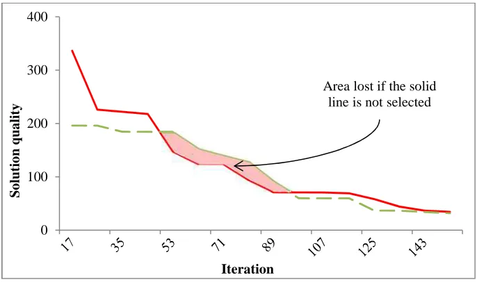
3.5 Area Lost as a secondary criterion for the Flexible-Budget method.

Assume a minimization problem 49

(10)

3.8

An example of allocating a budget between five parameter settings/systems withn0= 5. The numbers indicate the iteration in which a sample is taken. For

instance, systems 1 and 3 were sampled in the second iteration with system 1 being tested on instances 6-9, while system 3 was run on instance 6

51

3.9 A pseudo-code of the OCBA algorithm 53

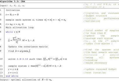
3.10 A pseudo-code of the CBA algorithm 55

3.11 Classification of the Racing algorithms used in this thesis 56

3.12 A pseudo code of a Racing algorithm 72

3.13 A pseudo code of a Racing algorithm with a reset 74

3.14 An example of Racing with reset 75

Chapter 4: Experiments, Results, and Analysis Meta-Optimization with a Flexible Budget

4.1

Comparison of the Fixed and Flexible Budget methods at different computational budgets. In this example, the Flexible Budget, using L, AUC,

or AL, was able to find a better (lower) solution quality at each of the four selected budgets less than 3000 (nmax)

79

4.2 Example instances of the hump function in 2D.Set-2 81

4.3 Example instances of the quadratic function in 2D.Set-3 82

Chapter 5: Experiments, Results, and Analysis Computational Budget Allocators

5.1 Comparison of different algorithms based onPICSunder 0.0

(above) and 0.9 (below) correlation._~_ࣨ (݅, 6ଶ₎_∀݅_{= 0, … ,}_{݇ −}₁ 109

5.2 Overall allocation of different algorithms at 0.0 and 0.9 correlation.

~ࣨ (݅, 6ଶ₎_∀݅_{= 0, … ,}_{݇ −}₁_{. The numbers are averaged over all replications} 111

5.3 Estimated mean of the best two systems under 0.0 correlation at selected

points throughout the run._~_ࣨ₍_݅_{, 6}ଶ₎_∀݅_{= 0, … ,}_{݇ −}₁ 114

5.4 Cumulative budget allocated to each system throughout the run, averaged over all replications._~_ࣨ ₍_݅_{, 6}ଶ₎_∀݅_{= 0, … ,}_{݇ −}₁. Correlation = 0.0 115

5.5 Cumulative budget allocated to each system throughout the run, averaged over

(11)

~ࣨ (݅, (݇ − ݅) )∀݅= 0, … ,݇ −1

5.7

Overall allocation of different algorithms at 0.0 and 0.9 correlation. ~ࣨ (݅, (݇ − ݅)ଷ₎_∀݅_{= 0, … ,}_{݇ −}₁_{. The numbers are averaged over all}

replications

118

5.8 Cumulative budget allocated to each system throughout the run, averaged over all replications._~_ࣨ₍_݅_{, (}_{݇ − ݅}₎ଷ₎_∀݅_{= 0, … ,}_{݇ −}₁. Correlation = 0.0

120

5.9 Cumulative budget allocated to each system throughout the run, averaged over all replications._~_ࣨ(݅, (݇ − ݅)ଷ₎_∀݅_{= 0, … ,}_{݇ −}₁_{. Correlation = 0.9} 122

5.10

Cumulative budget allocated to each system throughout the run, averaged over all replications._~_ࣨ₍_݅_{, (}_{݇ − ݅}₎ଷ₎_∀݅_{= 0, … ,}_{݇ −}₁_{. Correlation = 0.9.}

Only the systems getting less thann0are displayed

123

5.11 Comparison of different algorithms based onPICSunder 0.0

(above) and 0.9 (below) correlation._~_ࣨ ₍_݅_{, (}_݅_{+ 1)}ସ₎_∀݅_{= 0, … ,}_{݇ −}₁ 125

5.12

Overall allocation of different algorithms at 0.0 and 0.9 correlation. ~ࣨ(݅, (݅+ 1)ସ₎_∀݅_{= 0, … ,}_{݇ −}₁_{. The numbers are averaged over all}

replications

125

5.13 Cumulative budget allocated to each system throughout the run, averaged over all replications._~_ࣨ₍_݅_{, (}_݅_{+ 1)}ସ₎_∀݅_{= 0, … ,}_{݇ −}₁. Correlation = 0.0

127

5.14 Cumulative budget allocated to each system throughout the run, averaged over all replications._~_ࣨ(݅, (݅+ 1)ସ₎_∀݅_{= 0, … ,}_{݇ −}₁_{. Correlation = 0.9} 128

5.15 Cumulative allocations (a) byKW-RaceRR and convergence curves (b) based onPICSfor _~_ࣨ₍_݅_{, (}_݅_{+ 1)}ସ₎_∀݅_{= 0, … ,}_{݇ −}₁_{. Correlation = 0.9} 129

5.16 Comparison of different algorithms based onPICSunder 0.0 and 0.9 correlation (above) and (below)._~_{ࣨ ൫ܷ}_(0,_݇_),_ܷ_(10,24)_൯Set-A

131

5.17 Overall allocation of different algorithms at 0.0 and 0.9 correlation. ~ࣨ ൫ܷ(0,݇),ܷ(10,24)൯Set-A. The numbers are averaged over all replications

132

5.18 Cumulative budget allocated to each system throughout the run, averaged over all replications._~_{ࣨ ൫ܷ}_(0,_݇_),_ܷ_(10,24)_൯Set-A. Correlation = 0.0

134

5.19 Cumulative budget allocated to each system throughout the run, averaged over all replications._~_{ࣨ ൫ܷ}_(0,_݇_),_ܷ_(10,24)_൯Set-A. Correlation = 0.9

135

5.20 Box plots of the budget consumed byKW-Race at variousαvalues, and different correlation levels. The connecting line is that of the means

139

5.21 ECs based onfrat 0.0 (above) and 0.9 (below) correlation levels. Data are drawn from_~_ࣨ ₍_݅_{, 6}ଶ₎_∀݅_{= 0, … ,}_{݇ −}₁

141

5.22 ECs based onfrat 0.0 (above) and 0.9 (below) correlation levels. Data are

(12)

~ࣨ(݅, (݅+ 1) )∀݅= 0, … ,݇ −1

5.24 Weibull (left) and Gamma (right) distributions used inSet-3 experiments 146

5.25 Comparison of different algorithms based onPICSunder 0.0 (above) and 0.9 (below) correlation._~_ࣞ₍_݅_{, 6}ଶ₎_∀݅_{= 0, … ,}_{݇ −}₁

149

5.26 Overall allocation of different algorithms at 0.0 (a) and 0.9 (b) correlation.

~ࣞ(݅, 6ଶ₎_∀݅_{= 0, … ,}_{݇ −}₁_{. The numbers are averaged over all replications} 150

5.27 Cumulative budget allocated to each system throughout the run.~࣡(݅, 6ଶ)∀݅= 0, … ,݇ −1. Correlation = 0.0 (above) 0.9 (below) 151

5.28 Cumulative budget allocated to each system throughout the run.

~ࣱ (݅, 6ଶ₎_∀݅_{= 0, … ,}_{݇ −}₁_{. Correlation = 0.0 (above) 0.9 (below)} 152

5.29 Cumulative budget allocated to each system byKW-RaceRR throughout the

run. Correlation = 0.9. 153

5.30 Comparison of different algorithms based onPICSunder 0.0 (above) and 0.9

(below) correlation._~_ࣞ൫݅_{, 3(}_{݇ − ݅})൯∀݅= 0, … ,݇ −1 155

5.31 Cumulative budget allocated to each system throughout the run. ~ࣨ ൫݅, 3(݇ − ݅)൯∀݅= 0, … ,݇ −1. Correlation 0.0 (above) 0.9 (below)

156

~࣡൫݅, 3(݇ − ݅)൯∀݅= 0, … ,݇ −1. Correlation 0.0 (above) 0.9 (below) 157

~ࣱ ൫݅, 3(݇ − ݅)൯∀݅= 0, … ,݇ −1. Correlation 0.0 (above) 0.9 (below) 158

5.34 Comparison of different algorithms based onPICSunder 0.0 (above) and 0.9

(below) correlation._~_ࣞ൫݅_{, 4(}_݅_{+ 1)}_൯∀݅_{= 0, … ,}_{݇ −}₁ 161

5.35

Overall allocation of different algorithms at 0.0 (a) and 0.9 (b) correlation. ~ࣞ൫݅, 4(݅+ 1)൯∀݅= 0, … ,݇ −1.

The numbers are averaged over all replications

162

5.36 Cumulative budget allocated to each system throughout the run. ~ࣨ ൫݅, 4(݅+ 1)൯∀݅= 0, … ,݇ −1. Correlation 0.0 (above) 0.9 (below)

163

5.37 Cumulative budget allocated to each system throughout the run. ~࣡൫݅, 4(݅+ 1)൯∀݅= 0, … ,݇ −1. Correlation 0.0 (above) 0.9 (below)

164

~ࣱ ൫݅, 4(݅+ 1)൯∀݅= 0, … ,݇ −1. Correlation 0.0 (above) 0.9 (below) 165

5.39 Comparison of different algorithms based onPICSunder 0.0 (above) and 0.9 (below) correlation._~_ࣞ൫ܷ_(0,15),_ܷ_(20,40)_൯

(13)

~ࣨ ൫ܷ(0,15),ܷ(20,40)൯

~࣡൫ܷ(0,15),ܷ(20,40)൯. Correlation 0.0 (above) 0.9 (below) 169

~ࣱ ൫ܷ(0,15),ܷ(20,40)൯. Correlation 0.0 (above) 0.9 (below) 170

5.43 Estimated mean of the best four systems under 0.0 correlation at selected points throughout the run._~_{ࣨ ൫ܷ}_(0,15),_ܷ_(20,40)_൯ 171

5.44 Validation of CBA against published results based onPICS.

~ࣨ (݅, 6ଶ₎_∀݅_{= 1, … ,}_݇_. 176

5.45 Estimation of the covariance between system 0 and all other systems.

Estimation is made by CBA aftern0at 0.0 (a) and 0.9 (b) correlation 177

5.46 Box plots of the budget consumed byA-Race_2W at variousαvalues, and

different correlation levels. The connecting line is that of the means 180

drawn from_~_ࣨ ₍_݅_{, 6}ଶ₎_∀݅_{= 0, … ,}_{݇ −}₁_. 181

drawn from _~_ࣨ ₍_݅_{, (}_{݇ − ݅}₎ଷ₎_∀݅_{= 0, … ,}_{݇ −}₁ 182

drawn from _~_ࣨ(݅, (݅+ 1)ସ₎_∀݅_{= 0, … ,}_{݇ −}₁ 183

drawn from_~_{ࣨ ൫ܷ}_(0,_݇_),_ܷ_(10,24)_൯Set-A 184

drawn from_~_{ࣨ ൫ܷ}_(0,_݇_),_ܷ_(10,24)_൯Set-B 185

5.52 E[OC]for 0.0 (above) and 0.9 (below) correlation. Case 1 186

5.55 E[OC]for 0.0 (above) and 0.9 (below) correlation. Case 4,Set-A 189

5.56 Comparison of different algorithms based on_{b) and 0.9 (c and d) correlation. ~N(U(0,k),U(10,24))}PICSandE[OC]under 0.0 (a and_Set_-B 190

5.57 _{~N(U(0,k),U(10,24))}Overall allocation of different algorithms at 0.0 and 0.9 correlation._Set_{-B. The numbers are averaged over all replications} 191

(14)

5.60 E[OC]at 0.0 (left) and 0.9 (right) correlation for Case 1 194

5.61 E[OC]at 0.0 (left) and 0.9 (right) correlation for Case 4Set-A. 194

5.62 ECs based onfrand E[OC] at 0.0 (a and b) and 0.9 (c and d) correlation levels

for Case 4Set-B 194

5.63 E[OC]at 0.0 (left) and 0.9 (right) correlation for Case 3 195

(15)

degree of Doctor of Philosophy in Operational Research and Management Sciences. It has

been composed by myself and has not been submitted in any previous application for any

degree at any other university. All the work presented here, including the data and analysis,

was carried out by the author.

Parts of this thesis have been published:

1. Branke, J. and Elomari, J. A., 2012. Meta-optimization for parameter tuning with a

flexible computing budget. In:Soule, T. ed.Genetic and Evolutionary Computation

Conference.Philadelphia, 7-11 July. New York: ACM.

2. Branke, J. and Elomari, J., 2013. Racing with a fixed budget and a self-adaptive

significance level. In: Pardalos, P. and Nicosia, G. eds. Learning and Intelligent

(16)

Chapter 2: Literature Review

2.1 A sample comparison of the number of hyper-parameters required by some online controllers and the corresponding number of parameters to control 42

Chapter 3: Theory and Methodology

3.1 Data arrangement for a two-way ANOVA model 57

3.2 Data arrangement for a one-way ANOVA model 58

3.3 Data arrangement for a one-way ANOVA model with blocking 58 3.4 Test statistic calculations of a fixed effects two-way ANOVA model 61 3.5 Test statistic calculations of a fixed effects one-way ANOVA model

without blocking 62

3.6 Test statistic calculations of a fixed effects one-way ANOVA model_{with blocking} 62 3.7 Test statistic calculations of a mixed effects two-way ANOVA model 62 3.8 Effect of correlation on the actual_Nominal_αα_{= 0.05}values of a one-way ANOVA 63

3.9

Effect of heterogeneous variances on the actualαvalues of a one-way ANOVA model with various sample sizes

Nominalα= 0.05

64

3.10 Effect of heterogeneous variances on the actual α values of a one-way ANOVA 64

3.11 Effect of heterogeneous variances on the actual α values of a one-way ANOVA model with equal sample sizes (n1=n2= 10)

64

3.12 Effect of non-normality on the actualαvalues for a one-way ANOVA,

with different number of treatments and sample sizes 65 3.13 Effect of non-normality on the actual_{with different number of treatments and sample sizes}βvalues for a one-way ANOVA, 65

3.14 Effect of binomial data on the actualαvalues for a one-way ANOVA,

with various numbers of treatments and equal sample sizes 65 3.15 Effect of binomial data on the actual_{with different sample sizes and a constant number of treatments}βvalues for a one-way ANOVA, 66

3.16 Data arrangement for theF-test 68

(17)

No. Description Page 4.1 nmaxandbifor which parameters of CMA-ES are to be tuned 80

4.2

Comparison of the solution quality obtained by the Fixed and the Flexible Budget methods at various computational budgets, with α = 0.05

Results are forSet-1 functions

83

4.3 _{methods for}The best parameter settings proposed by the Fixed and Flexible Budget_Set_{-1. The numbers are averaged over all 30 replications of the} meta-EA

84

4.4

Comparison of the solution quality obtained by the Fixed and Flexible Budget methods at various computational budgets, with α = 0.05.

Results are for thehumpfunction in5Dwhere training and testing instances are different

87

4.5

Comparison of the solution quality obtained by the Fixed the Flexible Budget methods at various computational budgets, with α = 0.05.

88

4.6

Comparison of the solution quality obtained by the Fixed the Flexible Budget methods at various computational budgets, with α = 0.05.

89

4.7

Best parameter settings suggested by the Fixed and Flexible Budget methods. Highlighted cells indicate lowerµ/λratios proposed by the Flexible Budget.

Results are for thehumpfamily of functions in5D

91

4.8

92

4.9

92

4.10 _{dimensions for}Comparison of the best parameters proposed by each method across_Set_{-2. Results are limited to the 3000 budget case as it is the} only common case between all dimensions

93

4.11 Comparison of the solution quality obtained by the Fixed Budget method and_{the Flexible Budget method at various computational budgets, with}_α_{= 0.05.} Results are for the quadratic function in5D

94

95

(18)

Results are for thequadraticfamily of functions in5D

4.15

Best parameter settings suggested by the Fixed and Flexible Budget methods for various computational budgets.

97

4.16

Best parameter settings suggested by the Fixed and Flexible Budget methods for various computational budgets.

98

4.17 Comparison of the best parameters proposed by each method across

dimensions forSet-3. Results are for the 400 function evaluations budget 98

4.21 Computational effort savings gained by the Flexible Budget method over the

Fixed Budget method 100

4.22 _{better than (+), significantly worse than (-), or no significant difference than}Percentage of times the Flexible Budget method performed significantly (≈) the Fixed Budget method at α = 0.05

101

4.23 Computational effort savings gained by the Flexible Budget method over the Fixed Budget method

101

Chapter 5: Experiments, Results, and Analysis Computational budget allocators

5.1 Competing algorithms forSet-1 experiments 104

5.2 _Either_KW_{-Race or}Competing algorithms for_A_{-Race_2Way set the budget for OCBA, CBA, and EBA}Set-2 experiments. 104

5.3 LowestPICSand E[OC] achieved in Case 1 at 2000 samples for various

correlation levels 108

5.4

An example of why thePICSandE[OC]are at minimum near the end of an iteration. The best mean after each sample is shown inbold.

The data are drawn from_~_ࣨ ₍_݅_{, 6}ଶ₎_∀݅_{= 0, … ,}_{݇ −}₁_{with 0.9 correlation} 110

5.5 Variability in the average ranks assigned to each system by_{RaceRR, averaged over all replications. The}_NA_{indicates that no ranks were}F-RaceR andKW -assigned to that system beyondn0

(19)

5.7 _{The numbers based on all replications and are reported at the end of the run}Deviation of the estimated means from their nominal values. for_~_ࣨ(݅, (݇ − ݅)ଷ₎_∀݅_{= 0, … ,}_{݇ −}₁_{with 0.0 correlation}

117

5.8

Averages and variances of the ranks assigned to all systems byF-RaceR and KW-RaceRR. The numbers are based on all replications for _~_ࣨ (݅, (݇ − ݅)ଷ₎_∀݅_{= 0, … ,}_{݇ −}₁_{with 0.0 correlation. The numbers in}_bold_{represent the}

location of the largest gap in rank averages

119

5.9 Estimated mean of each system if it is sampled less, or more, than _ܰ_{௠ ௔௫}⁄_݇ 119

5.10 LowestPICSand E[OC] achieved in Case 3 at 2000 samples for various

correlation levels 124

5.11 The exact means and variances drawn from_~_{ࣨ ൫ܷ}_(0,_݇_),_ܷ_(10,24)_൯ ₁₃₀

5.12 LowestPICSand E[OC] achieved in Case 4,Set-A, at 2000 samples for

various correlation levels 131

5.13 _{0.9 correlation. The numbers are reported at the end of the run, and are based}Deviation of the estimated means from their nominal values, under 0.0 and on all replications._~_{ࣨ ൫ܷ}_(0,_݇_),_ܷ_(10,24)_൯.Set-A

133

5.14 LowestPICSand E[OC] achieved in Case 4,Set-B, at 2000 samples for

various correlation levels 136

5.15 _{0.9 correlation. The numbers are reported at the end of the run, and are based}Deviation of the estimated means from their nominal values, under 0.0 and on all replications._~_{ࣨ ൫ܷ}_(0,_݇_),_ܷ_(10,24)_൯.Set-B

136

5.16 A summary of the best performing algorithms (based onPICS) inSet-1

experiments 137

5.17 A summary of thefrachieved by the competing algorithms at selectedα

points of an EC. Data are drawn from_~_ࣨ(݅, 6ଶ₎_∀݅_{= 0, … ,}_{݇ −}₁ 140

points of an EC. Data are drawn from_~_{ࣨ ൫ܷ}_(0,_݇_),_ܷ_(10,24)_൯. Set-A 141

points of an EC. Data are drawn from_~_{ࣨ ൫ܷ}_(0,_݇_),_ܷ_(10,24)_൯. Set-B 141

points of an EC. Data are drawn from_~_ࣨ₍_݅_{, (}_{݇ − ݅}₎ଷ₎_∀݅_{= 0, … ,}_{݇ −}₁ 142

points of an EC. Data are drawn from_~_ࣨ (݅, (݅+ 1)ସ₎_∀݅_{= 0, … ,}_{݇ −}₁ 142

(20)

5.24 Deviation of the estimated means, of systems 0-2, from their nominal values._{The numbers are based on}_KW_{-RaceRR allocations by the end of the run} under 0.9 correlation

147

5.25 Percentage of the budget allocated to each system by OCBA at the end of the

run. Data_~_ࣞ(݅, (݅+ 1)ସ₎_∀݅_{= 0, … ,}_{݇ −}₁ 159

5.26 A summary of the best performing algorithms (based onPICS) inSet-3

experiments 172

5.27 Validation of CBA against published results based onPICS.~ࣨ(݅, 6ଶ)∀݅=

1, … ,݇ 176

5.28 Validation of CBA against published results based onPICS.

~ࣨ ൫ܷ(1,݇),ܷ(10,24)൯ 176

5.29 _{A summary of the}_f_r_{achieved by the competing algorithms at selected}_α

points of an EC. Data are drawn from_~_ࣨ(݅, 6ଶ₎_∀݅_{= 0, … ,}_{݇ −}₁ 178

points of an EC. Data are drawn from_~_ࣨ ₍_݅_{, (}_{݇ − ݅}₎ଷ₎_∀݅_{= 0, … ,}_{݇ −}₁

178

5.31 _{A summary of the}_f_r_{achieved by the competing algorithms at selected}_α

points of an EC. Data are drawn from_~_ࣨ (݅, (݅+ 1)ସ₎_∀݅_{= 0, … ,}_{݇ −}₁ 178

points of an EC. Data are drawn from_~_{ࣨ ൫ܷ}_(0,_݇_),_ܷ_(10,24)_൯.Set-A

179

points of an EC. Data are drawn from_~_{ࣨ ൫ܷ}_(0,_݇_),_ܷ_(10,24)_൯.Set-B

179

Chapter 6: Conclusion

6.1 A summary of the best performing algorithms (based on PICS) inSet-1

experiments 200

experiments 201

(21)

(22)

Abbreviation Description Page of definition

ACO Ant Colony Optimization 1

AL Area Lost 48

ANN Artificial Neural Networks 25

ANOVA Analysis of Variance 8

AOS Adaptive Operator Selection 13

AOTA Adaptive Online Time Allocator 35

AP Adaptive Pursuit algorithm 14

A-Race

A Racing algorithm based on a normal-model ANOVA

test

31

A-Race_1WUB A Racing algorithm based on a normal-model 1-way

unbalanced ANOVA test

66

A-Race_2Way A Racing algorithm based on a normal-model 2-way

ANOVA test

66

A-RaceR_2Way Normal model-based 2-way ANOVA Race with Reset 75

A-RaceRR_1WUB Normal model-based 1-way ANOVA Race with Reset

and Resample (unbalanced)

75

ARIMA Autoregressive Integrated Moving Average 24

ARMA Autoregressive Moving Average 24

AUC Area Under the Curve 47

avBSF best-so-far average utility 47

BasicILS Basic ILS (a version of the ParamILS algorithm) 31

BP Back Propagation 25

CA Credit Assignment 13

(23)

CL-PSO Comprehensive Learning Particle Swarm Optimization 15

CMA-ES derandomized Evolution Strategy with Covariance

Matrix Adaptation

78

DbV Difference based Velocity update strategy 15

DE Differential Evolution 25

DMAB Dynamic Multi Armed Bandit 17

DP Dynamic Programming 18

E[OC] Expected Opportunity Cost 101

EA Evolutionary Algorithm 1

EBA Equal Budget Allocation 74

EbV Estimation based Velocity update strategy 15

ES Evolutionary Strategy 20

FocusedILS Focused ILS (a version of the ParamILS algorithm) 31

fr Failure rate 101

F-Race A Racing algorithm based on Freidman’s test 29

F-RaceR Non-parametric 2-way Freidman ANOVA Race with

Reset (balanced)

75

GA Genetic Algorithm 22

GE Grammatical Evolution 25

GP Genetic Programming 25

HRTS Hamming Reactive Tabu Search 20

I\F-Race IteratedF-Race 30

ILS Iterated Local Search 18

KW Kruskal-Wallis test 8

KW-Race A Racing algorithm based on Kruskal-Wallis test 70

KW-RaceRR Non-parametric 1-way Kruskal-Wallis ANOVA Race

with Reset and Resample (unbalanced)

(24)

L Length 47

LL Lower Level algorithm 44

LSPI Least Squares Policy Iteration 19

LUS Local Unimodal Sampling 25

MAB Multi Armed Bandit 15

MCHH Markov Chain Hyper-heuristic 20

MMAS Max-Min Ant System 26

OCBA Optimal Computing Budget Allocation 33, 8

OPSO Optimized Particle Swarm Optimization 24

OS Operator Selection 13

ParamILS Parameter Iterated Local Search 31

PCS Probability of Correct Selection 51

PD Pareto Dominance 15

PICS Probability of Incorrect Selection 101

PM Probability Matching 14

PM-AdapSS-DE Probability Matching Differential Evolution with

Adaptive Strategy Selection algorithm

13

Pmin/Pmax Minimum/maximum selection probability 14

PR Pareto Rank 15

PS Parameter Setting 74

PSO Particle Swarm Optimization 15

QAP Quadratic Assignment Problem 26

REVAC Relevance Estimation and Value Calibration 37

RL Reinforcement Learning 19

RTS Reactive Tabu Search 19

(25)

SAT Boolean satisfiability problem 15

SD Steepest Descent 18

SMAC Sequential Model-based Algorithm Configuration 37

SMBO Sequential Model Based Optimization 35

SPO Sequential Parameter Optimization 36

STGP Strongly Typed Genetic Programming 26

TB-SPO Time Bounded Sequential Parameter Optimization 36

TS Tabu Search 1

TSP Traveling Salesman Problem 23

UCB1 Upper Confidence Bound algorithm 17

(26)

CHAPTER 1 Introduction

1.1. Motivation and problem statement

This thesis focuses on the algorithm configuration problem. Many search

algorithms, and metaheuristics in particular, have several parameters that affect their

performance in terms of solution quality and running time. Population size in Evolutionary

Algorithms (EA), tabu list length in Tabu Search (TS), and evaporation rate in Ant Colony

Optimization (ACO) are examples of numerical parameters, while parent and survival

selection types in EAs are examples of categorical parameters. Incorrectly setting these

parameters can, in extreme cases, cause the algorithm to behave greedily, converging early

to a local optimum. Or, it may behave similar to a random walk, where it does not converge

to any solution in the allowed time limit. In either case, computational effort is wasted on

poor quality solutions (De Jong, 2007). Ideally, the algorithm should explore as much as

possible before converging to high quality solution(s). See Figure1.1.

Figure 1.1. Effect of different parameter settings on an algorithm’s performance applied to a minimization problem.

120 170 220 270 320 370 420

S

o

lu

ti

o

n

q

u

a

li

ty

Iteratioin

(27)

Informally, the algorithm configuration problem is defined as: finding parameter

values which enable the algorithm to reach its best possible performance within the available

computational budget. Specifying what is “best” depends on the application, it could be, for

instance, the solution quality obtained within a time limit (or computational budget), the

running time needed to reach a target solution quality, or the percentage of how often a

stochastic algorithm reaches a target solution quality under a budget constraint.

Hutter (2009, pp. 9-12) formally defines the problem as a 6-tuple〈޿,߆, Π,ߢ_{௠ ௔௫}_,ߧ,߬〉

where: Αis a stochastic algorithm,Θ is the parameter space which includes the solution to

the algorithm configuration problem,Πis the set of problem instances, often generated from

a distribution D, κmax is the maximum cap time an algorithm is allowed to run, ο is the

observed performance of the algorithm, and τis a statistical measure (e.g. mean or median)

of the observed performance that is to be optimized.

1.2. Solution approaches

Setting the parameters of an algorithm is not trivial. There are many challenges that

require innovative methods to address them. This section first presents the major challenges,

and then moves to a broad description of the solution approaches.

First, an algorithm can have categorical and/or numerical parameters (continuous

and/or discrete), some of which can be conditional (i.e. they exist only if others do). For

example, crossover rate and tournament size are only relevant for an EA if a crossover

operator and a tournament selection are used, respectively. The parameter space is made up

of all possible combinations of parameter values, and its landscape (defined later) is likely to

be discontinuous and highly multi-modal, such that exhaustive search may not be feasible

(Eiben and Smit, 2011).

Second, evaluating a parameter’s quality, utility hereafter, on stochastic algorithms

may require several replications, which raises the question of how many replications are

(28)

depend on the budget available for assessment. A greedy parameter setting can seem

superior under a small budget compared to an explorative one. The situation may be

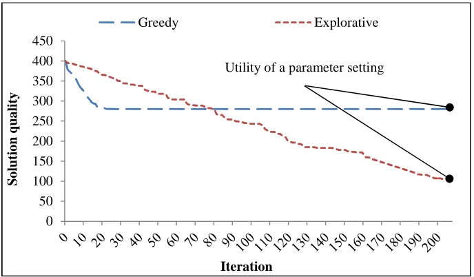
reversed if more time is allowed for the latter, see Figure1.2. This presents the challenge of

specifying the budget needed to evaluate a parameter setting.

Figure 1.2. Different parameter settings are suitable for different budgets.

For a minimization problem, a greedy parameter is suitable for small budgets, but not larger ones.

Third, parameter settings which work well on one problem domain, routing for

example, may not work for another, like cutting stock. The same issue extends across

instances of the same domain if they differ greatly, or even within the same instance

depending on its landscape. A problem domain encloses all instances (realizations of the

problem) that share common similarities. Measuring similarities depends on the problem

itself. For example, in a vehicle routing problem the number of nodes, their distribution

(scattered, clustered, or random), and the number of vehicles can be used to distinguish

between various instances. Smith-Miles and Lopes (2011) present several measures to

characterize many real-world optimization problems, and assess their difficulty.

If the problem is to be solved only once, it is desirable to find a parameter setting

which works best for that specific problem. Conversely, if similar problems, or instances, are

to be solved repeatedly, a parameter setting which performs well overall might be preferred. 0

50 100 150 200 250 300 350 400 450

0 20 40 60 80 100 120 140 160 180 200

S

o

lu

ti

o

n

q

u

a

li

ty

Iteration

(29)

also point out that finding a good generalist is by itself a multi-objective optimization

problem, with each problem, or instance, being one objective.

Solving the algorithm configuration problem requires another algorithm, working at

a higher level, and capable of searching the parameter space. EAs are an example. To

distinguish between both, the higher level algorithm will be referred to as the configurator

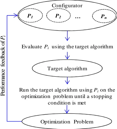
and the lower level algorithm as the target algorithm, see Figure 1.3 .The solutions of the

configurator are parameter settings suitable for the target algorithm. Some configurators

generate/modify parameter settings (e.g. through evolution as in EAs), while others only

select the best out of a given set. Note that the configurator is likely to be stochastic as well,

[image:29.595.223.416.345.557.2]

indicating that it, too, may require multiple replications.

Figure 1.3. Configuring parameters with a higher level algorithm.

Assessing a parameter’s utility requires running the target algorithm on the

optimization problem until a stopping condition, for that parameter, is met. A stopping

condition for a parameter can be, for example, a pre-specified number of iterations, the

continued application until no improvement is observed, or the continued application until

the target algorithm terminates. A performance measure is then fed back to the configurator

and used to determine the utility. Note that more than one performance measure can be

reported and combined in calculating a utility (e.g. running time and/or solution quality). Target algorithm

Optimization Problem

P1 P2 … Pn

EvaluatePi using the target algorithm

Run the target algorithm usingPion the

optimization problem until a stopping condition is met

P

er

fo

rm

an

ce

fe

ed

b

ac

k

o

f

Pi

(30)

The stopping condition for a parameter determines the frequency of feedback to the

configurator. One extreme is to report the performance only after the target algorithm

terminates, in which case multiple assessments require multiple complete runs of the target

algorithm on different instances of the optimization problem. The other extreme is to report

performance after one or more applications of a parameter (an operator) before the target

algorithm terminates, in which case the configurator gets feedback while the optimization

problem is being solved.

The former case will be referred to as offline tuningas parameter settings are learnt

after the problem is solved across many instances, and remain fixed. It is suitable for finding

a generalist based on a training set of instances that is assumed to be large enough and

representative, such that the best parameter setting found during training will also perform

best on other, unseen, test instances. The latter case will be referred to as online controlas

parameter settings are learnt, and hence change, while solving the problem. It is suitable for

finding a specialist.

Using online or offline rests on the application; does the problem require a specialist

or a generalist? It remains unclear, however, if a generalist can perform just as well as a

specialist, or if there is much to gain from online control over offline tuning. This issue will

be further addressed in Chapter 2, where a comprehensive overview of the state-of-the-art

configurators is presented, alongside a unique classification.

Finally, the termHyper-heuristicswas introduced just over a decade ago to refer to

high-level methods specializing in generating or selecting lower-level heuristics, or heuristic

components. The heuristics can be simple crossover or local search operators for example.

They can also be parameter settings for algorithms. Hyper-heuristics have little or no

problem domain knowledge, only information about the heuristics themselves; thus,

(31)

heuristic that is potentially able to solve a number of problem instances. Selective

hyper-heuristics, however, select and apply a heuristic to the current solution in order to improve it.

Comprehensive surveys on the topic are found in Burke et al. (2013) and in Chakhlevitch

and Cowling (2008).

Almost any configurator can be viewed as a hyper-heuristic. In this work, though,

the terms configurator, parameter setting/operator, and target algorithm will be used to

describe a framework for the algorithm configuration problem.

1.3. Contributions

The contributions are methodological. In specific, new efficient configurators are

introduced to tune algorithm parameters. This Section briefly describes each contribution,

the motivation behind it, and a summary of its experimental assessment results.

1.3.1. Meta-Optimization with a Flexible Budget

The first contribution concerns offline tuning, where the configurator modifies its

solutions to reach better ones. Such configurators are also known as meta-optimization

methods. Meta-optimizers are computationally intensive as evaluating a single parameter

setting requires a complete run of the target algorithm on the optimization problem. Also,

several replications, for both levels, may be required for stochastic algorithms. Matters

become worse if the computational budget for the target algorithm varies, because this will

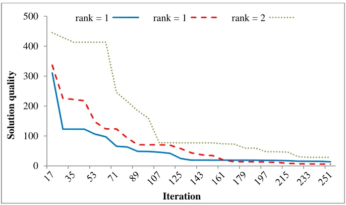
require a re-run of the whole meta-optimizer for each potential new budget. Figure 1.4

displays the performance of an algorithm, applied to a minimization problem, under three

different parameter settings. It is clear that the best parameter setting depends on the length

(32)

Figure 1.4. The performance of an algorithm, applied to a minimization problem, under three different parameter settings, each is suitable for a different computational budget.

This work proposes a new meta-optimizer capable of finding the best parameter

settings for any computational budget less than a specified maximum in a single run, thus

saving a lot of time. The algorithm is called Meta-Optimization with a Flexible Budget, or

Flexible Budget for short. It makes use of the entire convergence curve of a parameter

setting to calculate a rank-based utility.

It will be shown later that, for the experiments conducted here, the Flexible Budget

method always finds the best parameter settings for any computational budget less than a

specified maximum, while saving about 60%-70% of the computational effort required by

the repeated application of the Fixed Budget method, without compromising solution

quality. However, some experiments with a small budget using the quad function (defined

later), showed minor solution quality degradation. Further details are in Chapter 4. Initial

results of this method were presented in Branke and Elomari (2012).

A real-world application of the Flexible Budget is found in shipping. For next-day

parcel deliveries, the daily work load varies, which, in turn, affects the time needed to

prepare the parcels (e.g. inspection, weighing, sorting.). Such variability disturbs the running

time available to a routing algorithm dispatching vehicles on the next day. Obviously, with

only one to two hours at hand, the algorithm may perform better with a greedy parameter 0

50 100 150 200 250 300 350 400 450

0 20 40 60 80 100 120 140 160 180 200

S

o

lu

ti

o

n

q

u

a

li

ty

Iteration

(33)

1.3.2. Racing with a self-adaptive significance level

The second contribution also falls under offline tuning where the configurator

selects the best out of a set of parameter settings. There are a number of algorithms that

specialize in efficiently allocating a computational budget (e.g. a training set) among several

competing systems, the characteristics of which are unknown beforehand, such that the true

best is selected when the budget is consumed. These algorithms guarantee a correct selection

in the limit (i.e. if the budget is infinite), and converge to it at varying rates.

The term “system” is originally used in the Simulation Optimization literature to

refer to the performance of a simulated system (e.g. a production plant), which is usually

modeled with a probability distribution. Here, the term will be used to speak of the

performance of an algorithm, or a parameter setting over various problem instances.

Racing is one such algorithm. It works by discarding inferior systems, or parameter

settings, as soon as there is enough statistical evidence that they are significantly worse than

the current best. In every iteration, the surviving systems are sampled once and the tests are

run again. This continues until one system remains, or if the entire budget is consumed, in

which case the system with the best performance measure is chosen as the winner. The

algorithm’s performance (e.g. the probability of selecting the best) is affected by the

significance level α set by the user. A very high α results in less conservative tests and

increases the probability of discarding the true best as the systems are dropped off more

quickly. A very low α means more conservative tests, where the systems are hardly

discarded and the algorithm samples all systems almost equally.

Note that Racing may terminate before the entire budget is consumed. In situations

where there is a fixed budget constraint, such that there is no advantage of terminating the

algorithm beforehand, a new Racing algorithm, Racing with reset, is introduced. Its basic

idea is as follows: whenever a winner is identified and the budget is not entirely consumed,

(34)

significance level, and runs the tests on all systems. Consequently, if the best system was

incorrectly discarded before, it now has another chance to survive in the race. The process is

repeated as many times as needed until the budget is consumed. Racing with reset is thus

able to consume any given budget and at the same time automatically adaptα.

It will be shown later that Racing with reset, at a relatively highα(say 0.3), always

reaches a lower probability of incorrect selection (defined later), than its standard version

with the best fixed α set by the user. Moreover, if the variances of the parameter settings’

performance distribution are quite close, or they are highly correlated, its probability of

incorrect selection converges to zero faster than one of the best budget allocators from the

Simulation Optimization literature, namely the Optimal Computing Budget Allocation

(OCBA) algorithm, which addresses a problem similar to the focus of this thesis. See Chen

and Lee (2010). There are, of course, situations where Racing with reset is inferior (e.g. if

the variances are exponentially increasing), such situations will be detailed in Chapter 5.

Initial results of Racing with reset were presented in Branke and Elomari (2013).

1.3.3. One-way Racing with an intelligent budget allocation

All Racing algorithms currently used in the literature rely on a two-way Analysis of

Variance (ANOVA) test, so as to account for the effect of the parameter setting (first factor),

the effect of the problem instance (second factor), and their interaction. This, in turn, dictates

having an equal number of samples for each of the competing systems whenever the tests are

run, More importantly, every time a system is discarded, the remaining systems mustall be

sampled the same number of times (once is the default). This has two disadvantages, first, it

does not allow for a more intelligent way of allocating the budget in each iteration. Second,

it does not allow Racing with reset to use all previously collected data if the algorithm

terminates before the budget is consumed.

(35)

called KW-RaceR and can handle unequal sample sizes. To better allocate the budget in

every iteration, instead of sampling all surviving systems equally, OCBA is run to determine

the distribution of that iteration’s budget, utilizing all previous knowledge. This combination

allows for a different exploration vs. exploitation balance, compared to that obtained with

equal allocation (the default). It will be shown that such a combination causes KW-RaceR to

perform very similarly to OCBA.

1.4. Organization of the thesis

This thesis consists of six main chapters. Every chapter begins with an introduction

section stating its objectives and expectations, and finishes with a conclusion section

summarizing the main issues and findings. It is possible to grasp the main ideas of this thesis

just by reading these two sections of each chapter.

The most relevant work to the developed methods are reviewed in Chapter 2, with

the main objectives of positioning the before mentioned contributions within the literature,

and highlighting some areas that received little or no attention, and are believed to represent

future research topics. The theory and methodology of each contribution are detailed in

Chapter 3. Chapter 4 empirically validates the first contribution by comparing it to the

current methods in the literature and over a variety of scenarios. Chapter5does the same for

the second and third contributions. Finally, Chapter 6 summarizes what was presented and

(36)

CHAPTER 2 Literature Review

2.1 Introduction

The algorithm configuration problem has been recently advanced by different

research communities, and now there exists a wealth of literature describing various solution

approaches. Many of these approaches can be seen as extensions, or variations, of a few

ideas, and can hence be grouped under a common umbrella. This chapter identifies two such

key ideas, online control and offline tuning. It then organizes the current literature

accordingly, along with a constructive critique when possible. This classification will assist

in understanding how the current state-of-the-art methods have developed, and it helps

position the work presented in this thesis.

The chapter is organized as follows: Section 2.2 describes the basis for the

classification and the applications of each class. Section 2.3reviews the literature on online

control. Section 2.4 reviews the literature on offline tuning. Section 2.5 presents a few

experimental studies comparing both classes. Section 2.6 points to some research areas

which received little, or no, attention so far. Finally, Section2.7concludes this chapter.

2.2 Classification

Broadly speaking, algorithm configurators can be seen as online controllers, or

offline tuners. The difference being whether parameters change while the target algorithm is

solving the optimization problem, according to feedback from the search, or they remain

fixed. In both cases these parameter settings have to be learnt; online methods do it

on-the-fly, which makes them more likely to find specialized parameter settings for specific

(37)

makes them more likely to find generalized parameter settings suitable for instances similar

to the training set.

Eiben et al. (1999) distinguished between three types of online control:

deterministic, self-adaptive, and adaptive. Deterministic methods first learn a schedule of

parameter-changes based on a training set, and then apply these changes while the target

algorithm is running; hence, there is no feedback from the specific instance being solved.

Still, they can be considered as online controllers as the parameters change. Self-adaptive

methods are best seen in an EA context, where the parameter settings are encoded with the

solutions and evolve to better values. Whitacre et al.(2006) pointed out that such methods

increase the size of the search space, making the problem even harder to solve. Finally,

adaptive methods use performance feedback gathered during the search to determine which

operator to apply next.

A different sub-division of online control is proposed in this thesis, that is: single

step look-ahead methods, where the operator which is best for the next immediate move is

preferred, or multi-step look-ahead methods, where the operator which is bestn-steps ahead

is preferred. The latter assumes that while the immediate rewards of a chosen operator may

be less than those of the others, the gain expected n-steps ahead outweighs such smaller

losses.

Offline methods are sub-divided according to whether, or not, a model is built to

guide the search for the best parameter setting. The model represents a relationship between

the performance of an algorithm and a particular parameter setting. Model-free offline tuners

are further sub-grouped into meta-optimizers, or computational budget allocators that

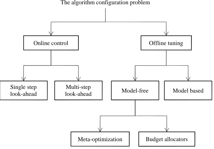
efficiently distribute a training budget among the competing parameters. Figure 2.1 shows

(38)

The application determines whether to use online or offline. If one is

interested in solving a single instance, a dynamic instance, or instances that are quite

different from one another, then online control is expected to discover a specialist for

that particular instance, without the need for the expensive training overhead

required by offline tuning, which may not be feasible to begin with. On the other

hand, if one is interested in solving many, similar, instances, then it may be

meaningful to invest once in offline tuning and find a generalist that works well on

many instances. In addition, offline tuning has the advantage of synthesizing

algorithm components, or even entire algorithms through Genetic Programming or

Grammatical Evolution.

Online control Offline tuning

The algorithm configuration problem

Single step look-ahead

Multi-step

look-ahead Model-free Model based

[image:38.595.141.498.78.326.2]

Meta-optimization Budget allocators

(39)

2.3 Online control

2.3.1 Single step look-ahead

Adaptive Operator Selection (AOS) methods are composed of two stages: Credit

Assignment (CA) and Operator Selection (OS). AOS applies an operator, from a set of

operators, to the target algorithm, observes its effect, assigns a reward to that operator based

on its performance, and finally selects an operator for the next iteration. The underlying

assumption is that the credit assigned to an operator, up until the current iteration, is

indicative of its future performance. Different CA and OS methods are available, and any

combination can be used.

The most basic CA method is based on solution quality observed during the last

iteration. A slightly advanced version considers the average quality, or a weighted average,

over the lastn iterations. Whitacreet al.(2006) were among the first to introduce the idea

that operators which produce rare, but large, improvements could be more beneficial than

those performing well on average. They setup an experiment to select the best out of ten EA

operators using five CA methods based on average performance, and two based on extreme

values. Results showed that the two extreme-value methods were significantly better than

the rest. However, they pointed out that if extreme improvements are very rare, it might be

better to focus on operators with steady improvements, especially towards the end of the run.

Extreme values were not always beneficial, for example Gonget al.(2010) applied

four CA methods to a Probability Matching Differential Evolution with Adaptive Strategy

Selection algorithm (PM-AdapSS-DE), they were: absolute reward, average normalized

reward, extreme absolute reward, and extreme normalized reward. PM-AdapSS-DE was

compared to a uniform selection DE and the Self-adaptive Differential Evolution algorithm

(SaDE) of Qinet al.(2009). PM-AdapSS-DE was able to outperform the others in terms of

solution quality and convergence speed when using average rewards instead of extreme