Sliding Mode Control, with Integrator, for a Class of
MIMO Nonlinear Systems
Anouar Benamor1, Larbi Chrifi-alaui2, Hassani Messaoud1, Mohamed Chaabane3
1Unit’e de Recherche en Automatique, Traitement du Signal et Image de l’ENIM, ATSI-ENIM, Monastir, Tunisie 2Laboratoire des Technologies Innovantes, Université de Picardie Jules Verne, Mitterrand, France
3Unité de Commande Automatique, l’Ecole Nationale d’Ingénieurs de Sfax, Sfax, Tunisie E-mail: [email protected], [email protected], [email protected],
Received January 24,2011; revisedMarch 8, 2011; accepted March 22, 2011
Abstract
In this paper, the robust control problem of general nonlinear multi-input multi-output (MIMO) systems is proposed. The robustness against unknown disturbances is considered. Two algorithms based on the Sliding Mode Control (SMC) for nonlinear coupled Multi-Input Multi-Output (MIMO) systems are proposed: the first order sliding mode control (FOSMC) with saturation (sat) function and the FOSMC with sat combined with integrator controller. Those algorithms were simulated and implemented on the three tanks test-bed system and the experimental results confirm the effectiveness of our control design.
Keywords: Sliding Mode Control, Integrator, Nonlinear Systems, Coupled, Mimo, Uncertain, Liquid Level Control
1. Introduction
The SMC is a widely used approach to design robust control law of uncertain systems. The advantage of such approach is its robustness to parameter variations and disturbances [1,2]. But the major inconvenience of clas-sic sliding mode control is the existence of chattering phenomenon [3], which may induce many undesirable oscillations in control signal. Some attempts on chatter-ing [4] cancelchatter-ing have considered continuous functions instead of sign one. However the provided results lead to a large steady state error which can be reduced using the integral action [5-7]. Moreover even though there exist many works dealing with sliding mode control in the case of Single Input Single Output (SISO) systems [8], there is lock of results when the addressed process is Multi-Input Multi-Output (MIMO) one. This shortage is due to output coupling problem.
In this paper, we propose a first order sliding mode control using Sat function and this control combined with an integrator corrector. Experimental results, oper-ated on a three tank system, are presented to illustrate the effectiveness of the proposed controllers.
The paper is organized as follows. In Section 2 we re-mind the classical sliding mode control of coupled MIMO
nonlinear systems and its robustness to parameter uncer-tainties and external disturbances. Section three is de-voted to SMC with sat function and integral action. The model of the coupled three tanks system and its control is presented in Section 4. The simulation and experimental results are presented in Sections 5 and 6. Finally Section 7 concludes the paper.
2. Sliding Mode Control
Consider a MIMO non linear system with p inputs and m outputs defined by the following state representation:
, ,
,
x f x t g x t u
y c x t
(1)
where x is the n-dimensional state vector and y is the m-dimensional output vector.
1
T n
x x x and is the
m-dimensional vector, the coefficients of which are nonlinear functions ci(x,t), f(x,t) is the n-dimensional vector, the coefficients of which are nonlinear functions fi(x,t), g(x,t) is a
1T m y y y
A. BENAMOR ET AL. 436 1 T p
u u u (2)
2.1. Classical Sliding Mode Control
Consider the sliding surface [9] defined by:
1
T p
s s s (3)
where:
1 0
, for 1, ,
i r
i k
i k i
k
s e i
p (4)with:
ri is the relative degree of the error ei i and for k = 1, , ri – 2,
1 1
i r
i k
are constants chosen so that
1
0 1 i
i r p
k
i i pri1is a Hurwitz polynomial one
and is the kth order derivative of the error e i. i
e
, 1, , 1.
d
i i i i
e y y i r (5)
where d i
y is the desired output. The derivative of si is:
1 0 1 d e d i r n i i i k
k j j
s ei
j x
t t x
(6)Replacing xj by its expression in (1) and omitting the index (x,t), relation (6) becomes.
1
0 1 1 1
d d
i
r n p n
i
i i i i
k j
k j j l j j
s e e e
jl l
f g u
t t x x
(7)which can be written as:
1 1 1 d d p i
i i iP P i il l
l s
h b u b u h b u
t
(8)with: 1 0 1 i r n
i i i
i k
k j j
s s h f t x
i and 1 0 1 i r n i i
ik k jl
k j j
s b g x
Then we can write the derivative of the surface vector as s h bu (9) with: 1 11 1 and P 1
P P P
h b h b h b P b b Theorem 1.
The control law for the first order sliding mode control (FOSMC) of the system 1 so that the sliding surfaces go to zero in a finite time is defined by:
1 1
1
P P
k sign s
u b h
k sign s
(10)
with ki a positive constant and b an invertible matrix. Proof.
Consider the following Lyapunov function:
21
1 1
2 2
T 2
P
V s s s s (11)
the derivative of V is:
1 1
T P P
Vs s s s s s (12) Using (9) we have:
T
Vs h bu (13)
Replacing u by its expression (10) in Equation (9), we obtain:
1 1
P P
k sign s s
k sign s
(14)
then
1 1 1 1 0 p P Ti i i i i
i i
P P
k sign s
V s k sign s s k s
k sign s
(15) Since ki (i = 1, , p) are positive we have V < 0. Then, the Lyapunov function V tends to 0 and there-fore all surfaces si tend to zero, hence the existence of the first order sliding mode.To prove the finite time convergence of our control we take the Equation (14), we have si k sign s si
i itheni i i i i i
s s k s s , with 0 ki,which is the reachability condition [10], then the finite time conver-gence.
2.2. Robustness to Parametric Uncertainties and External Disturbances
Consider an uncertain MIMO nonlinear system:
ˆ , , ˆ , ,
x f x t f x t g x t g x t u d (16)
where xnis the state vector, upis the input-control bounded as ui uimax for i = 1 to p, the vector field f x t
, f x tˆ
, f x t
,
is continuous and smooth, where f x tˆ
, is the nominal part and f x t
,is the uncertain part bounded by a known function. n
d D
no minal pa
represents the disturbances. The dynamic g(t,x
the no
) is t exactly known an rt
d it is written as the sum of
ˆ ,
with: ˆ ,
1 , ˆ , n ˆf x t f x t
f x t
,
ˆ ,
1 ˆ , ˆ , n f x t f x tf x t
, 1 n d d d
11 1 1ˆ , ˆ ,
ˆ ,
ˆ , ˆ ,
P
n nP
g x t g x t
g x t
g x t g x t
and
11 1 1 , , , , , P n nPg x t g x t
g x t
g x t g x t
Then the derivative of the sliding surface takes the following form:
1
d ˆ ˆ
d p i i s h
t i k ik ik k i
h b b u
(17)then:
ˆ ˆ δ
s h h b b u
1 ˆ , ˆ , ˆ , p h x t h x th x t
,
1 , , , p h x t h x th x t
, 1 δ δ δp
11 1 1ˆ , ˆ ,
ˆ ,
ˆ , ˆ ,
p
p pp
b x t b x t
b x t
b x t b x t
and Theorem 2.
Consider the uncertain system defined by Equation trol law:
(18)
with ki satisfying:
u (19)
and wher
11 1 1 , , , , , p p ppb x t b x t
b x t
b x t b x t
(16). The con
1ˆ ˆ
k sign s
1 1 P Pu b h
k sign s
* max 1 δ p
i i ik k
k
i k ei, ik, ties, te ti * δi 1 h , e
and are
of uncertai and respectively,
xpression of the derivative of the surface
be-max k
u
ik
b , δi rgenc
the upper bounds n
fi
conve k
ensures the ni m e of the sliding surface to zero. Proof. The e u comes:
ˆ ˆ δ
s h h b b u (20)
where s the p-dimensional vector wh are :
δi ose coefficients
1
δ n si d for 1 to
i j j j i p x
Using the control expression in (18) we ve: ha
1 1
k sign s
δP P
s h
k sign s
bu
(21)
The derivative of the surface si is then written:
δi i i i ik k i
s h k sign s b u
1
p
k
(22)
and the derivative of the Lyapunov function given by (12)
is:
1 i i
i
V s s
n
V eg
isfied
will be n ative if the following conditions are sat-: s si i 0 for i = 1 to p.
If si > 0 then si0, we have:
p
1
δ 0
i k i
k
h k
i b uik
(23)then i k 1 δ p
i ik k i
k
h b u
(24)If si < 0 then si0, we have:
1
δ 0
p
i k i
k
h u
i ik
k b
(25)then i k 1 δ p
i ik k i
k
h b u
(26)The conditions (24) and (26) are satisfied if:
* max δ
i ik ku i ki
1
p
k
(27)then
3. SMC with Sat
t of classic sliding mode control is e existence of chattering phenomenon. To avoid this
0
V
A. BENAMOR ET AL. 438
problem, we approximate the «sign» function by con-tinuous functions such as sat function [9] defined by:
sign s
i if si isat s
if
i i
i i
i s
s
28)
where
(
i
is a positive constant that defines the thickness of the ary layer.
he first order sliding mode control h sat of the system (1) is defined by: bound
Theorem 3.
The control law for t (FOSMC) wit
1 1
1
k sat s
u b h
P P
k sat s
(29)
with ki a positive constant and b an invertible matrix. Proof.
by n (11). Its derivative with using control defined in
We consider the same Lyapunov function defined Equatio
(31) is:
k sat s
1 1
T
P P
V s
k sat s
(30)
then
i
s (31)
Using sat definition given by (28), w
1p
i i
i
V k sat s
e have:
2
0 if
i i i i
sign s s s
0 if
i i i
i i
i
sat s s s
s
(32)
Therefore:
(33) then
(34) ark.
In the boundary layer the de
i i 0sat s s
0
V
Rem
rivative of the surface is:
i i
i
s s
(35)
then
e eri ri
i i
t t t t
i i ri i
s s t
(36)
with:
triis the start time of boundary layer. then
0 for 1,
i ri ,
s t t i p (37)
order to solve a steady-state error problem, an inte-gral sliding manifold was proposed in [10]
op
(38)
with In
. This devel-ment is introduced and justified only by tests on spe-cific systems. Our idea consists on reconstituting a con-trol law to eliminate steady-state error created by distur-bance. To do so we added an integral action when the trajectories of states approach their references [11-14]. Proposition.
Consider the uncertain system defined by Equation (1). aw FOSMC with integrator to eliminate The control l
steady-state error is defined by:
1 1
1
d
d
y y t
k sat s
1 1
1 1d d
P P
u b h K
k sat s y y t
11 1
1
p
p pp
K K
K
K K
The coefficients Kij are the integrator constant defined by:
j j
positive constant if d >
i i
y y
0 if
ij d
i i
K
y y
(39)
with
j
a positive constant.
cription and Modeling
tem, which ts on three
1
4. Validation
4.1. System Des
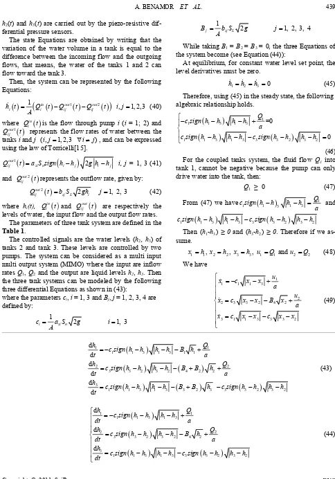
The considered process is a three tank sys ave two inputs and three outputs. It consis h
oming flow and the outgoing flo
h2(t) and h3(t)are carried out by the piezo-resistive dif-ferential pressure sensors.
The state Equations are obtained by writing that the variation of the water volume in a tank is equal to the difference between the inc
1 2 1, 2, 3, 4 j zj L
B b S g j
A
While taking B1 = B2 = B3 = 0, the three Equations of the system become (see Equation (44)):
At equilibrium, for constant water level set point, the level derivatives must be zero.
ws, that means, the water of the tanks 1 and 2 can flow toward the tank 3.
Then, the system can be represented by the following Equations:
1
in
out1
out2
, 1, 2,3 i t Qi t Qij t Qij t i j1 2 3 0
h h h (45) Therefore, using (45) in the steady state, the
algebraic relationship holds.
following
h A
(40)
1
1 1 3 1 3 =0
Q c sign h h h h
1 1 3 1 3 3 3 2 3 2 0
a
c sign h h h h c sign h h h h
where s the flow through pump i (i = 1; 2) and esents the flow rates of water betwee
, and can be expressed
in i
Q t i
repr and j ( ,e law o 1
out ij
Q t
tanks i
n the
(46) For the coupled tanks system, the fluid flow Q1 into tank 1, cannot be negative because the pump can dr
From (47) we have
1, 2,3 )
i j i j
using th f Torricelli[15].
1 out
ij zi i j
Q t a S h i, j = 1, 3 (41)
and Qout2
t represents the outfl 2 nsign h hi j g how rate, given by:
only ive water into the tank, then:
Q1 ≥ 0 (47) ij
2 2 1, 2, 3 (42) out
ij zj L i
Q t b S gh j
e hi(t),
1 1sign h1h 3 h1h3 a and
Q c
wher in
i
Q t and out
ijQ t are respectively the
levels of t fl e output
The parameters of three tank system are defi
ta
he system can be considered as a multi input m
water, the inpu ow and th flow rates.
ned in the c1sign h
1h3
h1h3 c sign h3
3h2
h3h2 Then (h1-h3)≥ 0 and (h3-h2)≥ 0. Therefore if we as-sume. [image:5.595.54.538.52.744.2]Table 1.
The controlled signals are the water levels (h2, h3) of nks 2 and tank 3. These levels are controlled by two
pumps. T x1h x1, , , 2h x2 3h u3 1Q1and u2Q2 (48) We h
ulti output system (MIMO) where the input are inflow rates Q1, Q2 and the output are liquid levels h2, h3. Then the three tank systems can be modeled by the following three differential Equations as shown in (43):
where the parameters ci, i = 1, 3 and Bj, j = 1, 2, 3, 4 are defined by:
ave
1
1 1 1 3
2
2 3 3 2 4 2
3 1 1 3 3 3 2
u
x c x x
a u
x c x x B x
a
x c x x c x x
(49)
1 2 1, 3 i zi n
c a S g i
A
1 1
1 1 3 1 3 1 1
2 2
3 3 2 3 2 4 2 2
3
1 1 3 1 3 3 2 3 3 3 2 3
d
d
d d d
d
h Q
c sign h h h h B h
t a
h c sign h h h h B B h Q
t a
h
c sign h h h h B B h c sign h h h h
t
2
(43)
1 1
1 1 3 1 3
2 2
3 3 2 3 2 4 2
3
1 1 3 1 3 3 3 2 3 2
d
d
d
h Q
c sign h h h h
dt a
h Q
c sign h h h h B h
dt a
h
c sign h h h h c sign h h h h dt
A. BENAMOR ET AL. 440
which can be written in the same form of (1) as:
,x f t x gu
y cx
(50)
where
1 2 3
Tx x x x ,
1 2
Tu u u ,
2 3
T y x x
1 1 3
3 3 4 2
1 1 3 3 3 2
,
f t x c x x B x
c x x c x x
c x x
,
1 0
a
1 0
g and
0 0
a
4.2. Sliding Mode Control of the Three Tank
System
The objective is to regulate the water levels of tank 2 and
tank 3 by using both laws defined in Section 3. The vector of the sliding surface is given by:
0 1 0 0 0 1 c
1 2
T s s swhere:
1 2 2d
s x x and s2
x3x3d
x3x3d
x2 2 and
tank n be
written as follows:
2
d and x3d are the desired water levels of tank 3. The derivative of the sliding surface $s_1$ ca
1 1 12
s l b u (51) with:
1 3 3 2 4 2 2d
l c x x B x x and 1 12 b
a
Similarly, the derivative of s2 is: 2 2 21 1 22 2
s l b u b u (52)
with:
1 1 3 3 3 2 1 1 3 3 3 2 4 22 2 1 1 3 3 3 2 3 1
1 2 d
l c x x c x x x c
x
3
3
2 x x 3
3 2
2 2
d
c x x c x x c x x c x x
c x
x
x B
22 3 1 2
b c
a x x
and 21 1
1 2
b c
a x x
3 2 3 1
then
s l bu (53) ith:
an
ontrol SMC with sat vector is:
with: w
1 2 l l
l
d b
12 21 22
0 b
b b
The C
1 12 2
k sign
u b l
k sign s
1 s (54)
3 1 3 2
c x x
1 3
1 1 1 3 2 1
1
0
ac x x a x x
c b
a
Control SMC with integrator vector is defined by:
(55)
with:
The
1 1
1 1
1
2 2 2 2
( ) ( )
d
d
y y dt
k sign s
u b l K
k sign s y y dt
11 12 21 22
K K
K
K K
5. Simulation Results
The controllers designed in Section 3 are simulated using the MATLAB software. The parameters of the three tank system Figure 1 are given in Table 1.The para eters for the both controls for three tanks are
m
0.6
, k1= 0.699, k2 = 0.53, K11 = 10−4, K12 = 18.10−3, K21 = 7.10−4 and K22 = −4
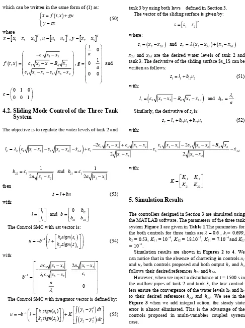
can notice that in the absence of chattering in controls u1 and u2 both controls proposed and both output h2 follows their desired references h2d and h3d.
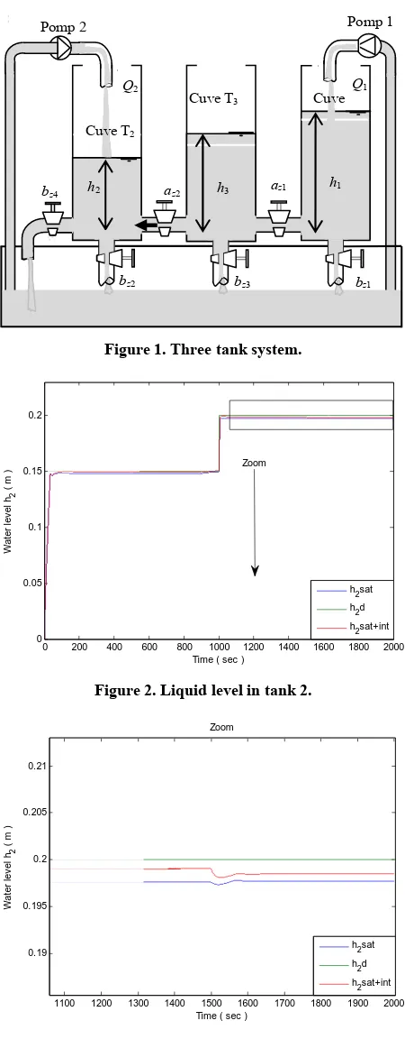
[image:6.595.52.539.71.723.2]ver, when we inject a disturbance at t = 1500 s in low pipes of tank 2 and tank 3, the tow control-lers ensure the convergence of the water levels h3 and h2 to their desired references h2d and 3d. We see in the Figure 3 when we add integral action, the steady state
This is the advantage of the -variables coupled system case.
10 .
Simulation results are shown in Figures 2 to 4. We
and h3
Howe the outf
h
az1
bz4 h2 h3 h1
bz3 bz1
bz2
Cuve T3 Cuve
Pomp 1
Q1
Cuve T2
Pomp 2
az2
Q2
Figure 1. Three tank system.
0 200 400 600 800 1000 1200 1400 1600 1800 2000 0
0.05 0.1 0.15 0.2
Time ( sec )
W
a
te
r le
v
e
l h
2
( m
)
h
2sat
h2d h
2sat+int
Zoom
Figure 2. Liquid level in tank 2.
1100 1200 1300 1400 1500 1600 1700 1800 1900 2000 0.19
0.195 0.2 0.205 0.21
Time ( sec )
Wa
te
r l
e
v
e
l h
2
(
m
)
Zoom
h
2sat
h2d h
[image:7.595.59.284.75.651.2]2sat+int
Figure 3. Liquid level with zoom in tank 2.
6. Experim
The proposed control algo ithms were tested on the physical laboratory plant (Figure 8) consisting of
inter-connected three tank system. The objective is to control the liquid level of tanks 2 and 3. The experimental schemes have been done under Matlab/Simulink, using Real-Time Interface, and run on the DS1102 DSPACE system, which is equipped by a power PC processor. The control algorithm is implemented on DSP (TMS 320C31).
ental Results
r
0 200 400 600 800 1000 1200 1400 1600 1800 2000 0
0.05 0.35
0.1 0.15 0.2 0.25 0.3
e
r le
v
e
l h
3
( m
)
Time ( sec )
W
a
t
h
3sat
h
3d
h
3sat+int
[image:7.595.311.536.172.347.2]Zoom
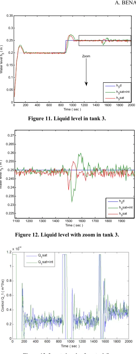
[image:7.595.308.540.389.705.2]Figure 4. Liquid level in tank 3.
Table 1. Numerical values for physical parameters of the three tank system.
Symbol Value Meaning
a 0.0154 m2 tank section
Sn 2.5 10−5 m2 cross-section of valve
aZi 0azi1 flow correction term (i = 1, 2, 3)
zi
b 0bzi1 leakage flow correction term (i = 1, 2, 3)
g 9.81 m/s2 gravity constant m/s2
hmax 0.6 m
maximum water level in each tank
(i = 1, 2, 3)
Qimax 1.17 10−4 m3/s maximum inflow through pump i (i = 1, 2)
1100 1200 1300 1400 1500 1600 1700 1800 1900 0.23
0. 32 0.27
5 0.24 0.245 0.25 0.255 0.26 0.265
Time ( sec )
W
a
te
r le
v
e
l h
3
(
m
)
[image:7.595.307.539.389.711.2]h3sat h3d h3sat+int
A. BENAMOR ET AL. 442
[image:8.595.62.282.52.608.2]0.22
Figure 6. Input signals of control Q1.
Figure 7. Input signals of control Q2.
Figure 8. Real system. The parameters for both controls for
three tanks are: ,
.10−5and
k1= 0.46, k2 = 0.32, K11 = 10−3, K12
= 3.10−4, K
21 = 11 K22 = 7.10−4.
For given references we remark that water levels h2d and h3d reach their references without overshooting. When we change the references we obtain the same re-sponse. In order to test the robustness of our strate
with respec urbances,
gy t to parameter uncertainties and dist
0 200 400 600 800 1000 1200 1400 1600 1800 2000 0.02
0.04 0.06 0.08 0.1 0.12 0.14 0.16 0.18 0.2
Wat
e
r l
e
v
e
l h
2
( m
)
Time ( sec )
h
2d
h
2sat+int
[image:8.595.316.527.78.428.2]h2sat Zoom
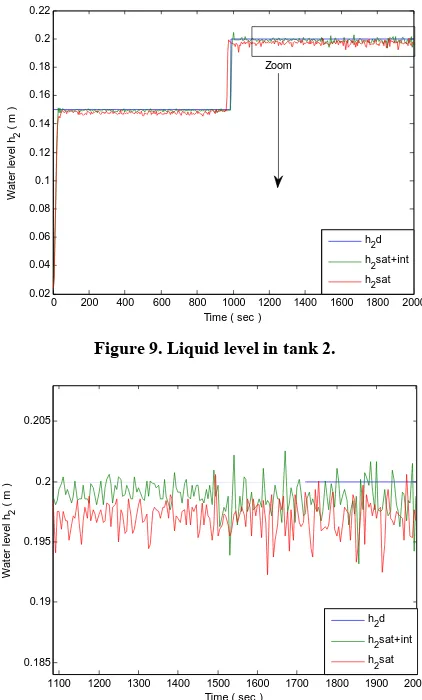
Figure 9. Liquid level in tank 2.
1100 1200 1300 1400 1500 1600 1700 1800 1900 2000 0.185
0.19 0.195 0.2 0.205
Time ( sec )
Wa
te
r l
e
v
e
l
h2
(
m
)
h2d
h2sat+int h2sat
Figure 10. Liquid level with zoom in tank 2.
we varied the parameters c1 and c3 by closing and open-ing a little bit the valves az1 and az2 and we introduce a permanent leakage in the outflow pipes of tank 2 and
tank 3 at t = the outflow
ipes of tank 2 and tank 3, the two controllers ensure the convergence of the water level h3 and h2 to their desired references h3d and h2d (Figures 9 and 11).
Then, the advantage of the sliding mode control with integrator in simulation and experimental results is the attenuation of error static (Figures 3, 5, 10, and 12).
Moreov er, we can also observe that control inputs Q1 and Q2 are smooth and the chattering phenomenon is almost eliminated (Figures 6, 7, 13 and 14).
7. Conclusion
In this paper, robust sliding mode control for a class of MIMO nonlinear systems was presented. In order
elimina state
rror ind s
slid-g mode control, combined with a conditional inteslid-grator 1500 s. We remark at 1500 s in
p
to te chattering phenomenon and the steady
uced by the use of sat function, continuou e
0 200 400 600 800 1000 1200 1400 1600 1800 2000 0
0.05 0.1 0.15 0.2 0.25 0.3 0.35
Time ( sec )
W
e
r le
v
e
l
h3
( m
)
a
t
h
3d
h
3sat+int
h
3sat
[image:9.595.64.283.58.628.2]Zoom
Figure 11. Liquid level in tank 3.
1100 1200 1300 1400 1500 1600 1700 1800 1900 0.225
0.23 0.235 0.24 0.245 0.25 0.255 0.26 0.265 0.27
Time ( sec )
W
a
te
r le
v
e
l h
3
( m
)
h
3d
h3sat+int h3sat
Figure 12. Liquid level with zoom in tank 3.
Figure 13. Input signals of control Q1
admittance coefficients of various pipes, leakage in the tanks and uncertainty due to neglected pump dynamics. was proposed. This control was applied to the level
control ench
ark. T w
ro-ustness to parameter variations such as tank Section, s -of MIMO nonlinear three tanks system b he simulation and experimental results sho m
b
Figure 14. Input signals of control Q2.
[1] V. Utkin, “Sliding Mode in Control and Optimization,” Springer-Verlag, Berlin, 1992
[2] V. Utkin, J. Guldner and J. Shi, “Sliding Modes Control in Electromechanical Systems,”CRC press, Boca Raton, 1999. [3] L. Fridman, “An Averaging Approach to Chattering,”
IEEE Transactions on Automatic Control, Vol. 46, No. 8, 2001, pp. 1260-1265. doi:10.1109/9.940930
The simulation and experimental results, compared with those obtained without integrator, confirm the ef-fectiveness of our control strategy.
7. References
[4] H. Abid, M. Chtourou and A. Toumi, “Robust Fuzzy Sliding Mode Controller for Discrete Nonlinear Sys-tems,” International Journal of Computers, Communica-tions and Control, Vol. 3, No. 1, 2008, pp. 6-20. [5] S. Mahieddine-Mahmoud, L. Chrifi-Alaoui, V. van
Ass-che, J.-M. Castelain and P. Bussy, “Sliding Mode Control Based on Field Orientation for an Induction Motor,”
IEEE Industrial Electronics Society, IECON, North Caro-lina,
6-] H. Hashimoto, H. Yamamoto, S. Yanagisawa and F. 20 November 2005, pp. 181-186.
[6
Harashima, “Brushless Servo Motor Control Using Vari-able Structure Approach,” IEEE Transactions on Industry Applications, Vol. 24, No. 1, 1988, pp. 160-170.
doi:10.1109/28.87267
[7] I. Eker and S Integral Augm
. A. Akinal, “Sliding Mode Control with ented Sliding Surface: Design and Ex-perimental Application to an Electromechanical System,”
Electrical Engineering, Vol. 90, No. 3, 2008, pp. 189-197.
doi:10.1007/s00202-007-0073-3
[8] A. Levant, “Chattering Analysis,” IEEE Transactions on Automatic Control, Vol. 55, No. 6, 2010, pp. 1380-1389.
doi:10.1109/TAC.2010.2041973
[image:9.595.314.529.74.253.2]A. BENAMOR ET AL. 444
echani-Prentice-Hall International, New Jersey, 1991.
[11] I. Eker snd S. A. Akinal, “Sliding Mode Control with Integral Action and Experimental Application to an Elec-tromechanical System Application to an Electrom cal System,” IEEE-ICSC Congress on Computational In-telligence Methods and Applications, Istanbul, 2-14 De-cember 2005, p. 6. doi:10.1109/CIMA.2005.1662303
[12] S. Seshagiri and H. K. Khalil, “Robust Output Feedback Regulation of Minimum-Phase Nonlinear Systems Using Conditional Integrators,” Automatic,Vol. 41, No. 1, 2005, pp. 43-54. doi:10.1016/j.automatica.2004.08.013
[13] R. Benayache, L. Chrifi-Alaoui, P. Bussy and J. M. Cas-
telain, “Sliding Mode Control with Integral Corrector: Design and Experimental Application to an Intercon-nected System,” Mediterranean Conference on Control
and Automation, Thessaloniki, 24-26 June 2009, pp.
831-836. doi:10.1109/MED.2009.5164647
[14] T. Floquet, S. K. Spurgeon and C. Edwards, “An Output Feedback Sliding Mode Control Strategy for MIMO Sys-tems of Arbitrary Relative Degree,” International Journal of Robust and Nonlinear Control, Vol. 21, No. 2, 2010, pp. 119-133. doi:10.1002/rnc.1579