Logistic and SVM Credit Score Models Based on Lasso Variable Selection

(1)

ISSN Online: 2327-4379 ISSN Print: 2327-4352

DOI: 10.4236/jamp.2019.75076 May 27, 2019 1131 Journal of Applied Mathematics and Physics

Logistic and SVM Credit Score Models Based on

Lasso Variable Selection

Qingqing Li

College of Science, University of Shanghai for Science and Technology, Shanghai, China

Abstract

There are many factors influencing personal credit. We introduce Lasso tech-nique to personal credit evaluation, and establish Lasso-logistic, Lasso-SVM and Group lasso-logistic models respectively. Variable selection and parame-ter estimation are also conducted simultaneously. Based on the personal cre-dit data set from a certain lending platform, it can be concluded through ex-periments that compared with the full-variable Logistic model and the step-wise Logistic model, the variable selection ability of Group lasso-logistic model was the strongest, followed by Lasso-logistic and Lasso-SVM respec-tively. All three models based on Lasso variable selection have better filtering capability than stepwise selection. In the meantime, the Group lasso-logistic model can eliminate or retain relevant virtual variables as a group to facilitate model interpretation. In terms of prediction accuracy, Lasso-SVM had the highest prediction accuracy for default users in the training set, while in the test set, Group lasso-logistic had the best classification accuracy for default users. Whether in the training set or in the test set, the Lasso-logistic model has the best classification accuracy for non-default users. The model based on Lasso variable selection can also better screen out the key factors influencing personal credit risk.

Keywords

Credit Evaluation, Logistic Algorithm, SVM Algorithm, Lasso Variable Selection

1. Introduction

In the 21st century, with the rapid development of China’s economy, the concept of Chinese people’s consumption has undergone tremendous changes, and the credit industry has developed rapidly. Among them, the development of credit

How to cite this paper: Li, Q.Q. (2019) Logistic and SVM Credit Score Models

Based on Lasso Variable Selection. Journal

of Applied Mathematics and Physics, 7, 1131-1148.

https://doi.org/10.4236/jamp.2019.75076

Received: April 22, 2019 Accepted: May 24, 2019 Published: May 27, 2019

http://creativecommons.org/licenses/by/4.0/

(2)

DOI: 10.4236/jamp.2019.75076 1132 Journal of Applied Mathematics and Physics

card business is increasing day by day, and the credit risk that comes with it is not to be underestimated. Credit scoring model has been the core of credit risk management. In fact, the credit scoring model is a statistical model that analyzes a large number of customers’ historical data, extracts key factors affecting credit risk, and then constructs a suitable model to evaluate the credit risk of new ap-plicants or existing customers. Therefore, the construction of the personal credit scoring model can respond to credit risk in a timely and effective manner, which will play an important role in both banks and regulatory authorities.

In this era of information explosion, however, the emergence of big data has also led to some credit information, and the existing scoring models often can-not effectively screen out dangerous customers. At the same time, the increasing of the high customer information can lead to the complexity of the credit scoring, model bias and instability, thus variable selection becomes the key issues and difficulties in personal credit evaluation model. It is of great significance to apply the variable selection method to the development of the credit scoring model. In the credit scoring model, the subset selection such as stepwise regression is a discrete and unstable process, and the variable selection will be changed by small changes in the data set. Selection and parameter estimation also need to be car-ried out in two steps. Subsequent parameter estimation does not take into ac-count the bias caused by variable selection, and accordingly it underestimates the actual variance. The calculation of subset selection is also quite complicated. In view of these defects, we adopt the Lasso method which can simultaneously perform variable selection and parameter estimation. After quantifying many explanatory variables, it is necessary to establish dummy variables as explanatory variables of the model. When using stepwise regression to select variables, only one dummy variable can be selected, which is the reason why the results are dif-ficult to explain. However, the above problems can be well solved by Group lasso when it performs variable selection on group variables, making the dummy va-riables belonging to the same group be completely retained or fully eliminated in the model.

In this paper, the Logistic and SVM models of Lasso were mainly used to se-lect and classify the influencing factors of personal credit evaluation. Then, the prediction accuracy of several models for default users is compared.

2. Literature Review

Typical credit evaluation models are: linear discriminant analysis, logistic re-gression, K-nearest neighbor, classification tree, neural network, genetic algo-rithm, support vector machine [1]-[7], etc. Among them, Logistic regression is most widely used in personal credit score, and support vector Machine (SVM) is a new artificial intelligence method developed in recent years. In 1980, Wiginton

(3)

machine method is obviously superior to the linear regression and neural net-work methods.

On the contrary, in China, the construction of the credit score system just started. Shi and Jin [9] summarize the main models and methods of personal credit score. Xiang [10] proposed to establish personal credit evaluation by using multiple discriminant analysis (MDA), decision tree, logistic regression, Bayes network (Bayes), BP neural network, RBF neural network and SVM. Shen and so on [11]did a follow-up study on support vector machines. Hu [12] believed that the most representative Logistic model are widely concerned by researchers due to its high prediction accuracy, simple calculation and strong variable explana-tory ability.

There are two main methods for selecting variables: subset selection method and coefficient compression method. Subset selection method is that in linear model, all variables form a set, and each subset of the set corresponds to a model. According to certain criteria, an optimal subset fitted regression model is se-lected from all subsets or partial subsets.

The main research on subset selection are AIC (Akaike Information Criterion)

[13] proposed by Akaike, BIC (Bayesian Information Criterion) [14] proposed by Scllwaz, CIC (covariance expansion criterion, Tibshirani and Knight) [15]

and Mallows’ C_P Guidelines [16]. Although these methods have strong practi-cability, there are many problems. For example: large algorithm complexity, high computational cost, poor interpretability of explanatory variables, etc.

(4)

which can not only select group variables but also select variables in a group is needed. That is the so-called, the so-called bi-level variable selection. After that, Huang et al.[25] proposed group bridge, and Simon et al.[26] proposed sparse group lass. All these are bi-level variable selection methods. The main contribu-tion of this paper is to apply Logistic, Lasso-logistic, Group lasso-logistic and Lasso-SVM models to evaluate personal credit scores. Through experimental comparison, the advantages of the progressive selection, the backward selection and the Lasso method in the selection of variables are compared, and the predic-tion accuracy of each model is also compared.

In the third section, we present the algorithm models of Lasso-logistic, Las-so-SVM and Group lasso-logistic, and propose the method to select the parame-ter lambda in the model. In the fourth section, with the help of the credit data of the credit platform, SPSS software is used to preprocess the data. Section five and six use R language to compare and analyze the variable selection ability and prediction accuracy of the model through numerical experiments, so as to draw relevant conclusions.

3. Model

3.1. Logistic Model

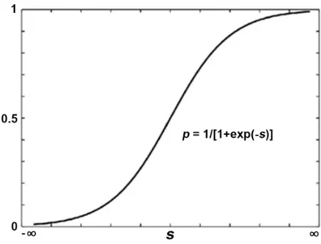
Logistic regression is a probabilistic nonlinear model, which is a multivariable analysis method used to study the relationship between binary observation re-sults and some influencing factors. Its basic idea is to study whether a result oc-curs under certain factors. For example, this paper uses some variable indicators to judge a person’s credit status. Logistic regression can be expressed as:

1 , 1 e s

P= ₋

+

0

1 . n

i i i

s β βx

=

= +

∑

where x i_i

(

=1,2, , n

)

is the explanatory variable in the credit risk assessment (or the characteristic indicator of the individual), β_i

(

i=1,2, ,_ n

)

_regression coefficient. Logistic regression value P∈

( )

0,1 _{is the discriminant result of}

cre-dit risk.

The graph of the function in Logistic regression model has an s type distribu-tion, as shown in Figure 1.

As you can see from Figure 1, P is a continuous increasing function of s,

(

,

)

s∈ −∞ +∞ , and:

1

lim lim 1,

1 e s s→+∞P=s→+∞ + − =

1

lim lim 0.

1 e s s→−∞P=s→−∞ + − =

For someone i i

(

=1,2, ,_ n

)

_{, if} P_i is close to 1 (or Pi ≈1), then it is judged

(5)

[image:5.595.264.489.70.241.2]

Figure 1. The graph of the logistic function.

then the person is judged to be “good”. That is, the value of Pi farther away

from 1 indicates that the person is less likely to fall into default set. On the con-trary, it means that the risk of default is greater.

Suppose there are data variables

(

x y i_i, _i

)

, =1,2, ,_ n_,

where xi =

(

x xi1, , ,i2  xim

)

which is the observed value of the explanatory

va-riable and y_i∈

{ }

0,1 _{is the observed value of the interpreted variable. In the}

general regression model, the observed values of the explanatory variable and the interpreted variable are often considered to be independent. In addition, assume that xij is standardized. Namely, 1 ij 0,1 ij2 1

i x i x

n

∑

= n

∑

= . Let

(

1|

)

i i i

P P y= = x be the conditional probability of yi =1 given xi. The

con-ditional probability under the same conditions is P y

(

i =0 |xi

)

= −1 Pi. Then,

given a test sample

(

x y_i, _i

)

, its probability is:

( )

(

)

1

1 i,

i y

y

i i i

P y =P −P −

where e0₀1 1_{1 1}

1 e

i m im

x x

i x x

P = ₊β_β+β+_β+ ++ +β_β



 . Assume that each sample is independent of each

other. Their joint distribution (i.e., likelihood function) can be expressed as:

(

)

(

)

1

0 1

1

, , , n yi 1 yi.

m i i

i

L β β β P P −

=

∏

−



The Maximum Likehood method is a good choice to estimate the parameter

β. Because it can maximize the possibility that the observed value of each sam-ple is equal to its true value. In other words, it can maximize the log likelihood function in the logistic model:

(

)

(

)

(

)

(

)

1 0 1 1 1

ln ( , , , ) ln 1

ln 1 e . i i

i

n _y

y

m i i

i n

X i i

i

L P P

y X β

β β β

β − = =   = _ − _   = − +

∏

∑



For convenience, we set X_i =

(

1,x_i

)

and

β

=

(

β β

0, , ,1

β

m

)

T. Estimating

(6)

solve the following problem:

( )

ˆ argmaxl ,

β = β

It is easy to know that l

( )

β is concave and continuously differentiable, and therefore its local maximizer is the global maximizer. Calculate partial deriva-tives and make it to be zero, which leads to the likelihood equations:

(

)

(

)

0 1 1

0 1

1 0

ln , , , _e

0, 1 e

i m im

x x

n m

i x x

i L

y β β_{β β} β_β

β β β

β + + + + + + = ∂   = _ − _= ∂

∑

_ + _   

(

)

(

)

0 1 1

0 1

1

ln , , , _e

0. 1 e

i m im

x x

n m

i x x ij

i j

L

y β_ββ_β β_β x

β β β

β + + + + + + = ∂   =  −  = ∂

∑

_ + _   

But it is difficult to get an explicit solution. It needs to be solved by some iter-ative methods such as Newton-Raphson, EM and gradient descent algorithms. The estimated

β

j obtained by the likelihood equation is called the maximum

likelihood estimate, and the corresponding conditional probability Pi is

esti-mated by Pi .

Logistic has a wide range of applications in credit scoring. The traditional Lo-gistic method is very simple, but it is sensitive to multi-collinearity interference between individual credit variables. Therefore, some redundant variables are se-lected, resulting in poor prediction results. That is why we improve this method.

3.2. Lasso Model

Tishirani proposed the Lasso method which is motivated by non-negative Gar-rote [27].

Let βˆ=

(

βˆ1, , βˆm

)

T, the estimator

( )

α βˆ, ˆ of the lasso method is:

( )

_, 2

1 1

ˆ

ˆ, arg min n i m j ij , s.t. m j ,

i y j x j t

α β

α β α β β

= =  _ _    = _ _ − − _ _ ≤     

∑



∑

where t≥0_{is the regularization parameter. For all}_t_{, one has an estimator}

ˆ y

α = of

α

. Without loss of generality, we assume that y=0, Above prob-lem can be rearranged into the following form:

2

1

ˆ argmin n i m j ij , s.t. j .

i y j x j t

β

β β β

=  _ _    = _ _ − _ _ ≤     

∑



∑

It can also be expressed in the form of the following penalty function:

2

1 1

ˆ argmin n i m j ij m j .

i y j x j

β

β β λ β

= =     _ _ = _ _ −  + _    _ _ 

∑



∑



∑



The first part of the formula represents the goodness of the model fit, and the second part represents the penalty of the parameter. The harmonic coefficient

[

0,

]

λ∈ +∞ _{is smaller. The smaller role of the penalty term plays the more}

(7)

3.2.1. Logistic-Lasso Model

The Lasso method is mainly applied to linear models. The essence is to add a penalty function to the sum of squared residuals. When estimating parameters, the coefficients are compressed, and some coefficients are even compressed to 0 to achieve model variable selection. But for credit default prediction, the depen-dent variable is a binary value. In this case, the linear regression model cannot be used. Instead, Lasso-logistic [28] should be used. Penalized logistic regression is a modification of the logistic regression model. The negative log-likelihood function adds a non-negative penalty term to achieve good control of the coeffi-cients.

The conditional probability of the logistic linear regression model can be ex-pressed as:

(

)

(

1|

)

( )

log ,

1 1|

i i

i

i i

P y x

x

P y x ηβ

 = 

 _{ =}

 ₋ ₌ 

 

 

where ηβ

( )

xi =Xiβ .

The coefficient estimate βλ in the Lasso-logistic regression model is given

by the minimum value of the convex function of the following form:

( )

1 ,

m j j

Sλ β l β λ β

=

= − +

∑

where

( )

{

( )

{

( )

}

1 log 1 exp

n

i i i

i

l β yηβ x ηβ x

=

 

=

∑

− + _ _

The estimator βˆ in Lasso-logistic regression model can be given as:

( )

{

( )

}

{

}

1 1

ˆ argmin n i i log 1 exp i m j .

i y β x β x j

β

β η η λ β

= =

 



= −

∑

− + _ +

∑

3.2.2. Lasso-SVM Model

The standard SVM model does not have feature selection capabilities. The spe-cific approach of adding regularization to the SVM model is to use the regulari-zation term with sparsity to replace the L2 norm in the standard SVM. The L1

norm is convex functions, with Lipschitz continuum, having properties better than other norms. L1-SVM and its similar extensions have evolved into one of

the most important tools for data analysis. The general form of Lasso-SVM is given below:

1 1

min m i n i

j Ci

β ξ

= =

+

∑

(

T

)

₁

s.t. y Xi i

β

≥ −

ξ

i, i=1,2, , n

0. i

ξ ≥

(8)

( )

1 1

min n 1 i i m i.

i y f X j

λ β + = =  −  +  

∑

where 1−y f Xi

( )

i ₊ is a Hinge loss function and λ is a regularization

pa-rameter.

3.2.3. Group Lasso-Logistic Model

Group lasso was introduced by Yuan and Lin (2006), allowing pre-defined cova-riates to be grouped together and selected from the model. All variables in a par-ticular group can be included or not included. It is very useful in many settings. Group lasso algorithm for logistic regression was first proposed by Kim et al., and then Meier et al.[29] proposed a new one which can solve high dimensional problems.

Suppose there is an independent and identical distribution of observation

(

x y i_i, _i

)

, =1,2, ,_ n_. x_i =

(

x x_i₁, , ,_i₂ _ x_im

)

_{which is an m-dimensional vector} that can be divided into G groups, and the dependent variable is a binary varia-ble y_i∈

{ }

0,1 _{. The independent variable can be a continuous variable or a}

clas-sified variable. Assume that the degree of freedom of the group g argument is

g

df , Xi =

(

1, ,x xi,1 i,2, , xi G,

)

,

(

g=1,2, , G

)

. xi g, denotes the xi g, group of

variables of the observation xi g, . Similarly, β can be expressed as

(

_{β β β}

0_{; ; ; ;}1 2 _

_β

G

)

_, _βg_{denotes the coefficients corresponding to group G g}

variables, where the labeling method is used to distinguish the

β

j fraction in

the case of no grouping. The probability of “default” of the dependent variable

( )xi

(

1| i

)

Pβ =P yβ = x can be expressed by the following model:

( ) ( )

( )

T 0 , 1 log , 1 i i G x

i i g g i

g x

P

x x X

P

β

β β

η β β β

=    _{ =} ₌ ₊ ₌  ₋     

∑

where β0 denotes intercept,

β

g is the coefficient vector corresponding to

group g and β is the whole coefficient vector.

The parameter β λˆ

( )

_{can be estimated by minimizing the convex function:}

( )

2

1 ,

G

g g

g

Sλ β l β λ s df β

=

= − +

∑

where l

( )

β is a logarithmic likelihood function:

( )

{

( )

{

( )

}

1 log 1 exp ,

n

i i i

i

l β yηβ x ηβ x

=

∑

− + _ _

( ) ( )

1 2

g g

s df = df _and s

( )

⋅ is used to rescale the parameter

β

g vector.

3.3. The Choice of Harmonic Parameter

(9)

The main idea of K-fold cross validation is that the data are randomly divided into K (usually 5 or 10) identical parts. Each k=1, ,_ K_{, uses the data of the}_K part as the test sample, and uses the remaining K-1 parts of the data as the training sample to fit the model. Loop K times until all k are traversed. We de-note the estimator by _βˆ−k_{. The harmonic parameter} _{β λ}ˆ

( )

_{corresponds to a}

classification model and the corresponding estimator β λˆ

( )

_{. The generalization}

error of each model corresponding to lambda is given by the mean square pre-diction error. That means Cross-Validation Error (CVE) is estimated:

( )

(

T

)

2

1

1 1 _ˆ _,

k K

k

i i

k ki

CV y X

K n

λ β−

= ∈

=

∑ ∑

−



where k is the k-th partial cross-check sample, nk = k = _Kn . Minimize the

above formula to find the most appropriate harmonic parameters, and the cor-responding model can be considered to be the model with the best performance based on cross-check error.

4. Data

4.1. Data Source

The original data is mainly from a domestic lending institution. There are a total of 8000 records in this data set, including 25 fields. Among them, 23 fields de-scribe the personal characteristics of the lender, including the basic personal identity information: domicile, gender, local work, education level and marital status. Also include personal economic ability: whether there is a CPF salary lev-el. Data set also includes personal debt and debt repayment record: frequency of personal housing loan, personal commercial housing loan pen number and fre-quency of other loan credit card account number, number, frefre-quency of delin-quent loans, loans overdue month loan highest monthly overdue amount, max-imum length, loan account number of the contract amount, loan balance has been used lines, the average individual loan maximum contract value, the aver-age individual loans minimum contract amount, the last six months on averaver-age use. Finally, the data set also gives the total number of times of individual ap-proval query and loan number. The result, where “0” is the performance cus-tomer and “1” is the default cuscus-tomer.

4.2. Data Preprocessing

(10)

pre-DOI: 10.4236/jamp.2019.75076 1140 Journal of Applied Mathematics and Physics

diction accuracy of the model for default customers with relatively small data capacity. Therefore, the under-sampling method is adopted for compliance users. That means some representative data are selected from the data with more sam-ples. In order to reduce the majority of the sample, the data balance is achieved. The final data set is divided into a training set and a test set, wherein the training set has 3002 data, including 1500 compliance data and 1502 default data, and the test set has 519 data including 258 compliance data and 261 default data.

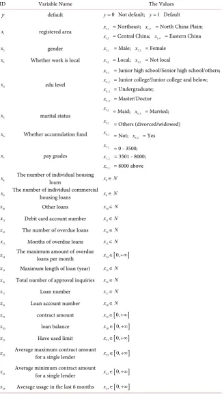
4.3. Variable Description

The classified and encoded variables in the data are shown in Table 1.

5. Numerical Experiment

The full-variable logistic and stepwise logistic regression models were imple-mented by using SPSS 22.0. The Lasso-logistic model was impleimple-mented by using the glmnet package in R language, the Lasso-SVM model was implemented by using the gcdnet package, and the Group lasso-logistic model was implemented by using grpreg. The code package uses the generalized coordinate descent me-thod [30] to calculate the model under regularization and its generalized solu-tion path.

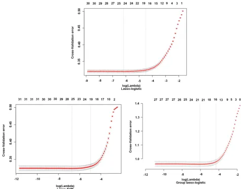
5.1. Parameter Lambda Selection

Through the K-fold cross-validation, the Lasso-logistic, Lasso-SVM, and Group lasso-logistic models are changed with the value of lambda, and the model error is changed. At the top of Figure 2, the number of corresponding variables se-lected by the model is given. The value between the two dotted lines in Figure 2

indicates the range of positive and negative standard deviation of lambda, and the dotted line on the left indicates lambda when the model error is minimized. Tibshirani contends that lambda takes a relatively small change in the model prediction bias within this interval. It is generally recommended to choose lambda which makes the model relatively simpler, namely, a large lambda within a standard deviation range. It is the best value. It can also be seen from Figure 2

that as the value of lambda changes, the degree of compression of the model va-riable also changes. In other words, the number of vava-riables to be filtered is af-fected by the estimate of lambda.

(11)

[image:11.595.213.542.91.667.2]

Table 1. Variable declaration.

ID Variable Name The Values

y default y=0 Not default; y=1 Default

1

x registered area x1,1 = Northeast; x1,2 = North China Plain;

1,3

x = Central China; x1 4， = Eastern China

2

x gender x2 1， = Male; x2.2 = Female

3

x Whether work is local x3,1 = Local; x3.2 = Not local

4

x edu level

4,1

x = Junior high school/Senior high school/others;

4,2

x = Junior college/Junior college and below;

4 3

x， = Undergraduate;

4,4

x = Master/Doctor

5

x marital status 5,1

x _{= Maid;}

5,2

x = Married;

5,3

x _{= Others (divorced/widowed)}

6

x Whether accumulation fund x6,1_{= Not;}

6,2

x = Yes

7

x pay grades

7,1

x _{= 0 - 3500;}

7 2

x， = 3501 - 8000;

7,3

x = 8000 above

8

x The number of individual housing

loans x8∈N

9

x The number of individual commercial _{housing loans} x9∈N

10

x Other loans x10∈N

11

x Debit card account number x11∈N

12

x The number of overdue loans x12∈N

13

x Months of overdue loans x13∈N

14

x The maximum amount of overdue

loans per month x14∈

[

0,+∞

]

15

x Maximum length of loan (year) x15∈N

16

x Total number of approval inquiries x16∈N

17

x Loan number x17∈N

18

x Loan account number x18∈N

19

x contract amount x19∈

[

0,+∞

]

20

x loan balance x20∈

[

0,+∞

]

21

x Have used limit x21∈

[

0,+∞

]

22

x Average maximum contract amount _{for a single lender} x22∈

[

0,+∞

]

23

x Average minimum contract amount

for a single lender x23∈

[

0,+∞

]

24

x Average usage in the last 6 months x24∈

[

0,+∞

]

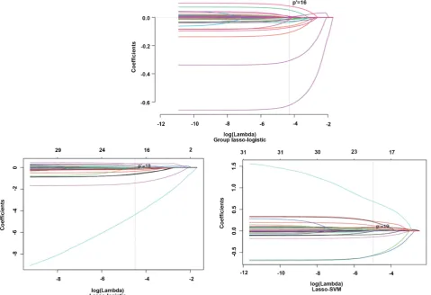
5.2. Coefficient of the Models

(12)

[image:12.595.56.532.73.445.2]

Figure 2. Lambda corresponds to the number of variables.

accordingly, which means the probability for judging credit as 1 (i.e., default) increases. When the coefficient βi is negative, it means that the variable xi

has a reverse restrictive effect on the default. When the coefficient βi is

posi-tive, the corresponding variable xi has a positive effect on the default, and the

greater the value of βi, the greater the promoting effect of the corresponding i

x on the customer’s credit judgment as default. In full-variable logistic model, the variable x6 (Whether accumulation fund), x11 (Debit card account number),

x14 (The maximum amount of overdue loans per month), x22 (Average maximum

contract amount for a single lender), x13 (Average minimum contract amount

for a single lender) before the coefficients were not significant, which means the model contains too many variables, and the model is too complicated. The above non-significant variables were eliminated by stepwise regression. At the same time, x18 (Loan account number) and x21 (Have used limit) were also eliminated.

(13)

[image:13.595.59.539.77.405.2]

Figure 3.Lasso coefficient solution path.

model. The Lasso-SVM model eliminates 15 variables, leaving 19 variables. However, it can be seen that when using stepwise regression, Lasso-logistic and Lasso-SVM models for variable selection, the variables are excluded as classifica-tion variables, and some dummy variables in the same group are partially re-tained and partially eliminated, such as x4 (edu level), which makes the result

difficult to explain, showing in Table 2.

Using Group lasso, after variable selection, 18 variables were removed and 16 variables were retained. In addition, Group lasso-logistic can retain or eliminate related dummy variables of the same group as a whole, making the dummy va-riables have explanatory significance. We obtained from the coefficient table of the Group lasso model that in the regional variable (x1), the north China area is

the high default area, and the central China area has the lowest default risk. There was a significant gender (x2) difference in credit risk that the default

probability of male was generally higher than that of female. In the salary scale (x7), people with low incomes were more at risk of default than those with

me-dium and high incomes. In historical credit records, customers with overdue loans are at greater risk of default, and the number of overdue loans (x12) and

months of overdue loans (x13) are more likely to default. More total number of

(14)

[image:14.595.206.537.90.724.2]

Table 2. Model coefficient table.

Variate Full variables Forward Backwards Lasso-logistic Lasso-SVM Group-lasso

X1_1 1.715 0 1.721 0 −0.555 0.025

X1_2 1.674 0 1.695 0.010 −0.567 0.001

X1_3 −4.562 −4.247 −4.561 −4.354 0.667 −6.520

X1_4 −1.534 −1.681 0 −1.440 0.016 −1.637

X2 −0.868 −0.854 −0.858 −0.630 0.209 −0.824

X3 −0.497 −0.504 −0.502 −0.352 0.122 −0.471

X4_1 1.408 0.341 0.501 0.105 −0.003 0.207

X4_2 0.780 0.301 0.218 0 0 −0.007

X4_3 0.575 0 0 −0.111 0.015 −0.195

X4_4 0.761 0 0 0 0 −0.682

X5_1 −0.025 −0.002 0 0 0 0.062

X5_2 −0.179 0 −0.201 −0.037 0 −0.072

X5_3 −0.034 0 0 0 0 0.073

X6 0.072 0 0 0 0 0.065

X7_1 0.306 0.393 0.311 0.355 −0.085 0.570

X7_2 −0.893 0.205 −1.111 −0.582 0.226 −0.554

X7_3 0.934 0 0 0 0 0.251

X8 0.123 0.101 0.098 0 0 0

X9 0.058 0 0 0 0 0.039

X10 −0.265 −0.213 −0.212 −0.104 0.053 −0.194

X11 −0.078 0 0 −0.003 0.013 −0.016

X12 −0.100 −0.111 −0.109 −0.084 0.033 −0.108

X13 −0.190 −0.206 −0.197 −0.064 0.050 −0.170

X14 −0.033 0 0 0 0 −0.021

X15 0.130 0.121 0.119 0 −0.016 0.101

X16 0.455 0.459 0.457 0.306 −0.142 0.431

X17 0.222 −0.218 −0.209 −0.173 0.084 −0.179

X18 0.164 0 0 0 0 0

X19 −0.405 0 0 −0.021 0 −0.062

X20 0.276 0 0 0 0 0

X21 0.136 0 0 0 0 0

X22 0.065 0 0 0 0 0

X23 0.041 0 0 0 0 0.035

X24 −0.325 −0.249 −0.263 −0.178 0.067 −0.212

Intercept

(15)

coefficient 0 indicate that they have been removed from the model and have lit-tle effect on credit rating.

Showing in Table 2, the number of the full-variable logistic model is the larg-est, and the complexity of the model is the largest. The forward and backward models excluded 13 explanatory variables, while the Lasso-logistic model ex-cluded 16 variables, three more than the stepwise selection. The number of Las-so-SVM excluded variables was 15, one less than the Lasso-logistic model, and two more than the stepwise selection. The Group lasso-logistic model had the strongest ability to eliminate variables, with 18 variables removed. It can also be concluded that in the selection of the same group of dummy variables, the Group lasso-logistic model retains or removes the entire group of variables, making the model variables have explanatory significance.

5.3. Model Prediction Accuracy

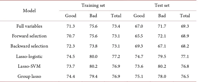
In the actual credit risk assessment, the misclassification of default users into non-defaulting users is more of a potential loss to banks or society. Therefore, the model is more important for to correctly classify the default users than to take non-defaulting users into consideration. It is easy to see in Table 3 that in the training set, the Lasso-SVM model predicts that the number of default users will be up to 80.16%, which is 4.53% higher than the full-variable model and is higher than the stepwise forward and backward selections 6.59% and 6.39% re-spectively. The Lasso-logistic and Group lasso-logistic models also predicted the default users could reach 79.96% and 80.09% respectively; in the test set, the Group lasso-logistic model got the best prediction on default users, reaching 80.62%. It is higher than the full-variable, forward and backward models 8.97%, 14.34%, 13.57% respectively, and the Lasso-SVM model is the second most ac-curate for the default user. The Lasso-logistic model follows. Next, look at the classification of non-defaulting users. Lasso-logistic is the best rate in both the training set and the test set. The forward selection model had the worst predic-tion accuracy for non-defaulting users. In the overall predicpredic-tion accuracy, the stepwise selection performed poorly in the test set. Lasso-logistic reached 77.21% in the training set, and Group lasso-logistic model has the highest overall predic-tion rate in the test set, reaching 77.26%.

6. Conclusions

In the personal credit evaluation, the Logistic model is most widely used, and the newly proposed SVM method in statistical learning also has certain application in credit evaluation. By comparing the simulation experiment analysis, the whole variable, Forward selection, Backward selection, Lasso-logistic, Las-so-SVM, and Group lasso-logistic models and empirically analyzing the personal credit data of a domestic lending platform, it can be concluded:

(16)

[image:16.595.208.541.89.227.2]

Table 3. Model prediction rate.

Model Training set Test set

Good Bad Total Good Bad Total

Full variables 71.3 75.6 73.4 67.0 71.7 69.3

Forward selection 70.7 75.6 73.1 65.5 72.1 68.9

Backward selection 72.3 73.8 73.1 69.3 67.1 68.2

Lasso-logistic 74.5 80.0 77.2 74.7 79.5 77.1

Lasso-SVM 73.7 80.2 76.9 73.6 80.2 76.8

Group lasso 74.4 79.4 76.9 75.1 78.0 76.5

the significant level test. Thus, to some extent, the complexity of the model was increased. The interpretability of the model was reduced. The choice and Lasso overcome the multicollinearity of the full-variable model, and the coefficients of the insignificant variables in the model are compressed. Compared with the stepwise regression, the Group lasso-logistic culling variable is the strongest, followed by Lasso-logistic, Lasso-SVM model. The algorithm model based on Lasso variable selection can better select important variables, and Group las-so-logistic will retain the whole group or the entire group when the same group of dummy variables is selected, which will enhance the variables in the model to some extent.

Second, in the training set, the Lasso-SVM model has the highest prediction accuracy rate for default users; in the test set, Group lasso-logistic ranks the first in the classification accuracy of default users. Whether in the training set or in the test set, the best classification accuracy of non-defaulting users is the Las-so-logistic model. Moreover, in the training set, the overall prediction accuracy of the Lasso-logistic model is also the best. In the test set, the Group las-so-logistic model has the best overall prediction accuracy. Regardless of the pre-diction of defaulting users, the prepre-diction of non-defaulting users and the overall forecasting accuracy, Lasso is better than stepwise selection. It shows that the credit scoring model based on Lasso variable selection has good extrapolation.

Therefore, based on the Logistic and SVM models established by the Lasso va-riable selection method, the explanatory vava-riables can be selected more scientifi-cally and have use value in personal credit risk assessment, which can well re-duce personal credit risk.

(17)

in personal credit risk assessment and can well reduce personal credit risk. In future work, we will consider individual credit ratings for unbalanced da-tasets. When we use Group lasso for intra-group variable selection, the coeffi-cient of some individual variables within the Group may not be significant. In this case, the two-layer variable selection is introduced to solve such problems.

Conflicts of Interest

The author declares no conflicts of interest regarding the publication of this pa-per.

References

[1] Eisenbeis, R.A. (1978) Problems in Applying Discriminant Analysis in Credit Scor-ing Models. Journal of Banking & Finance, 2, 205-219.

https://doi.org/10.1016/0378-4266(78)90012-2

[2] Henley, W.E. (1995) Statistical Aspects of Credit Scoring. Ph.D. Thesis, Open Uni-versity, Milton Keynes.

[3] Chatterjee, S. and Barcun, S. (1970) A Nonparametric Approach to Credit Screen-ing. Journal of the American Statistical Association, 65, 150-154.

https://doi.org/10.1080/01621459.1970.10481068

[4] Breiman, L.I., Friedman, J.H., Stone, C.J. and Olshen, R.A. (1984) Classification and Regression Trees (CART). Biometrics, 40, 874.

https://doi.org/10.2307/2530946

[5] Jensen, H.L. (1992) Using Neural Networks for Credit Scoring. ManagerialFinance, 18, 15-26. https://doi.org/10.1108/eb013696

[6] Desai, V.S., Crook, J.N. and Overstreet Jr., G.A. (1996) A Comparison of Neural Networks and Linear Scoring Models in the Credit Union Environment. European Journal of Operational Research, 95, 24-37.

https://doi.org/10.1016/0377-2217(95)00246-4

[7] Van Gestel, T., Baesens, B., Garcia, J. and Van Dijcke, P. (2003) A Support Vector Machine Approach to Credit Scoring. Bank en Financiewezen, 2, 73-82.

[8] Wiginton, J.C. (1980) A Note on the Comparison of Logit and Discriminant Models of Consumer Credit Behavior. The Journal of Financial QuantitativeAnalysis, 15, 757-770. https://doi.org/10.2307/2330408

[9] Shi, Q.-Y. and Jin, Y.-Y. (2004) A Comparative Study on the Application of Various Personal Credit Scoring Models in China. Statistical Research, 21, 43-47.

[10] Xiang, H. and Yang, S.-G. (2011) New Developments in the Study of Key Tech-niques for Personal Credit Scoring. The Theory and Practice of Finance and Eco-nomics, 32, 20-24.

[11] Shen, C.-H., Deng, N.-Y. and Xiao, R.-Y. (2004) Personal Credit Evaluation Based on Support Vector Machine. Computer Engineering and Applications, 40, 198-199. [12] Hu, X.-H. and Ye, W.-Y. (2012) Variable Selection in Credit Risk Analysis Model of

Listed Companies. Journal of Applied Statistics and Management, 31, 1117-1124. [13] Akaike, H. (1973) Information Theory and Extension of the Maximum Likelihood

Principle. In: Parzen, E., Tanabe, K. and Kitagawa, G., Eds., Selected Papers of Hi-rotugu Akaike, Springer, New York, 267-281.

(18)

DOI: 10.4236/jamp.2019.75076 1148 Journal of Applied Mathematics and Physics 6, 461-464. https://doi.org/10.1214/aos/1176344136

[15] Tibshirani, R. and Knight, K. (1999) The Covariance Inflation Criterion for Adap-tive Model Selection. Journal of the Royal Statistical Society, 61, 529-546.

https://doi.org/10.1111/1467-9868.00191

[16] Mallows, C.L. (1973) Some Comments on Cp. Technometrics, 15, 661-675.

https://doi.org/10.2307/1267380

[17] Hoerl, A.E. and Kennard, R.W. (1970) Ridge Regression: Applications to Nonor-thogonal Problems. Technometrics, 12, 69-82.

https://doi.org/10.1080/00401706.1970.10488635

[18] Frank, I.E. and Friedman, J.H. (1993) A Statistical View of Some Chemometrics Regression Tools. Technometrics, 35, 109-135.

https://doi.org/10.1080/00401706.1993.10485033

[19] Tibshirani, R. (1996) Regression Shrinkage and Selection via the Lasso. Journal of the Royal Statistical Society, Series B, 58, 267-288.

https://doi.org/10.1111/j.2517-6161.1996.tb02080.x

[20] Efron, B., Hastie, T., Johnstone, I. and Tibshirani, R. (2004) Least Angle Regression.

The Annals of Statistics, 32, 407-499. https://doi.org/10.1214/009053604000000067

[21] Zou, H. (2006) The Adaptive Lasso and Its Oracle Properties. Journal of the Ameri-can Statistical Association, 101, 1418-1429.

https://doi.org/10.1198/016214506000000735

[22] Yuan, M. and Lin, Y. (2006) Model Selection and Estimation in Regression with Grouped Variables. Journal of the Royal Statistical Society, 68, 49-67.

https://doi.org/10.1111/j.1467-9868.2005.00532.x

[23] Wang, L., Chen, G. and Li, H. (2007) Group SCAD Regression Analysis for Micro-array Time Course Gene Expression Data. Bioinformatics, 23, 1486-1494.

https://doi.org/10.1093/bioinformatics/btm125

[24] Huang, J., Breheny, P. and Ma, S. (2012) A Selective Review of Group Selection in High-Dimensional Models. Statistical Science, 27, 481-499.

https://doi.org/10.1214/12-STS392

[25] Huang, J., Ma, S., Xie, H. and Zhang, C.-H. (2009) A Group Bridge Approach for Variable Selection. Biometrika, 96, 339-355.

https://doi.org/10.1093/biomet/asp020

[26] Simon, N., Friedman, J., Hastie, T. and Tibshirani, R. (2013) A Sparse-Group Lasso.

Journal of Computational & Graphical Statistics, 22, 231-245. https://doi.org/10.1080/10618600.2012.681250

[27] Breinman, L. (1995) Better Subset Regression Using the Nonnegative Garrote.

Technometrics, 37, 373-384. https://doi.org/10.1080/00401706.1995.10484371 [28] Fang, K.-G., Zhang, G.-J. and Zhang, H.-Y. (2014) Personal Credit Risk Warning

Method Based on Lasso-Logistic Model. The Journal of Quantitative & Technical Economics, 2, 125-136.

[29] Meier, L., Van De Geer, S. and Bühlmann, P. (2008) The Group Lasso for Logistic Regression. Journal of the Royal Statistical Society, 70, 53-71.

https://doi.org/10.1111/j.1467-9868.2007.00627.x