ISSN Online: 2327-4379 ISSN Print: 2327-4352
DOI: 10.4236/jamp.2019.71001 Jan. 7, 2019 1 Journal of Applied Mathematics and Physics
Analytical Solution of Van Der Pol’s Differential
Equation Using Homotopy Perturbation Method
Md. Mamun-Ur-Rashid Khan
Department of Mathematics, University of Dhaka, Dhaka, Bangladesh
Abstract
In this research work, Homotopy perturbation method (HPM) is applied to find the approximate solution of the Van der Pol Differential equation (VDPDE), which is a well-known nonlinear ODE. Firstly, the approximate solution of Van Der Pol equation is developed using Dirichlet boundary con-ditions. Then a comparison between the present results and previously pub-lished results is presented and a good agreement is observed. Finally, HPM method is applied to find the approximate solution of VDPDE with Robin and Neumann boundary conditions.
Keywords
Homotopy Perturbation Method (HPM), Van Der Pol Differential Equation (VDPDE), Nonlinear Differential Equations, Analytic Solution,
Boundary Conditions
1. Introduction
The Van Der Pol differential equation [1] can be written as
(
2 1)
0y u y′′+ − y y′+ =
(1.1) where, u is a scalar parameter. It is considered as an example of an oscillator with nonlinear damping, energy being dissipated at large amplitudes and gener-ated as low amplitude. Such systems typically possess limit cycles: sustained os-cillations around a state at which energy generation and dissipation balance [1] [2]. The main application by VDP models an electric circuit with a triode valve, the resistive properties of which change with current, the low current, negative resistance becoming positive as current increases. This model has been widely applied in science and engineering [3]. The parameter u is indicating the nonli-nearity and the strength of the damping.
How to cite this paper: Khan, Md.M.-U.-R. (2019) Analytical Solution of Van Der Pol’s Differential Equation Using Homotopy Per- turbation Method. Journal of Applied Ma-thematics and Physics, 7, 1-12.
https://doi.org/10.4236/jamp.2019.71001
Received: November 20, 2018 Accepted: January 4, 2019 Published: January 7, 2019
Copyright © 2019 by author(s) and Scientific Research Publishing Inc. This work is licensed under the Creative Commons Attribution International License (CC BY 4.0).
DOI: 10.4236/jamp.2019.71001 2 Journal of Applied Mathematics and Physics The concept of HPM was first established by He [4] [5], which has been used to solve a large number of non-linear problems. It is found that such approxima-tions rapidly converges to the exact solution [4] [5]. Since it is not easy to find the solution of Equation (1.1) by usual methods such as the perturbation method, separation of variables etc., HPM can be used to find the analytical solution of nonlinear differential equations with different types of initial and boundary con-ditions [6] [7] [8] [9]. “In addition, the merging of perturbation method and the homotopy method is called homotopy perturbation method [4] [5], which has banished the deficiency of the traditional perturbation methods. On the other hand, this method can use the full benefit of perturbation techniques.”
2. Formulation of HPM
The details of the following formulation is given in He which is presented below: Consider the following non-linear differential equation [5]:
( ) ( )
0,M y q x− = x∈
φ
(2.1)
with
, y 0, ,
N y x
n
∂
= ∈ Φ ∂
(2.2)
Here, M has two parts (linear and nonlinear), Ln and Nln respectively. Then re-write Equation (2.1) as
( )
( ) ( )
0Ln y +Nln y q x− = (2.3) Then He [4] [5] introduced a homotopy g r t
( )
, :φ
×[ ]
0,1 → which satisfy( ) (
, 1)
( )
( )
0( ) ( )
0,[ ]
0,1 ,H g t = −t Ln g −Ln v +t M g q x − = t∈ x∈
φ
(2.4a) which is equivalent to( )
,( )
( )
0( )
0( ) ( )
0H g t =Ln g −Ln v +tLn v +t Nln g −s x =
(2.4b)
It follows from Equation (2.4a) and Equation (2.4b) that
( )
,0( )
( )
0 0H g =Ln g −Lln v = (2.5)
( )
,1( ) ( )
0H g =R g q x− =
(2.6) “Thus, the changing process of t from zero to unity is just that of g x t
( )
, from v x0( )
to g x( )
. In topology, this is called deformation, and( )
( )
0Ln g −Lln v , M g q x
( ) ( )
− are called homotopic.” [4] [5]Here, t is very small and assume that
2
0 1 2
g g tg t g= + + + (2.7) Setting t=1, approximate solution of Equation (2.1) can be obtained as,
0 1 2
DOI: 10.4236/jamp.2019.71001 3 Journal of Applied Mathematics and Physics
3. Numerical Examples
In Example 1, the VDPDE with Dirichlet boundary conditions is solved by HPM and comparisons between the HPM and exact solutions are presented here after.
Example 1:
(
2 1)
0,( )
0 0,( )
20 1y u y′′+ − y y′+ = y = y =
Considering y′′ +y as the linear part and u y
(
2−1)
y′ as the nonlinear partwe get the following Homotopy,
(
) (
)
(
2)
0 0 0 0 1 0
Y Y′′+ − y′′+y +t y′′−y +t u Y − Y′=
(3.1)
Putting,
[ ] [ ]
2
0 1 2, 0 csc 20 sin
Y Y tY t Y y= + + = x ,
in Equation (3.1) and equating the coefficients of t from both sides, we get
( )
( )
0 0 0
0 0, 0 0, 20 1
y′′ +y = y = y =
( )
( )
1 1 02 0 0 0, 1 0 0, 1 20 0
y y uy y uy′′+ + ′− ′= y = y =
( )
( )
2 2 0 1
2 2 0 1 0 1 0, 2 0 0, 2 20 0
y′′+y + uy y y uy uy y′− ′+ ′= y = y =
Solving we get,
[ ] [ ]
0 csc 20 sin
y = x
[ ]
[ ]
(
(
[ ]
)
[ ]
[ ]
[ ]
)
3
1 161 csc 20 sin 40 2 4cos 40
80cos 40 sin 40 sin 2
y u x x
x = − + − + − +
[ ]
(
[ ] [ ]
[ ]
[ ] [ ]
[ ] [ ]
[ ] [ ]
[ ]
[ ]
[ ] [ ]
[ ]
[ ] [ ]
[ ]
[ ]
[ ]
[ ]
[ ]
3 2 2 2 2 2 2 2 21 csc 20 18cos 5 cot 20 3072
144cos 20 cos 40 sin 960cot 20 sin 48 cot 20 sin 24cot 20 sin
12cos 40 cot 20 sin 12cos 80 cot 20 sin 9600csc 20 sin 960 csc 20 sin
y u x
x x
x x x
x x
x x x
= − + − + − − − − +
[ ]
[ ]
[ ] [ ]
[ ]
[ ]
[ ]
[ ]
[ ]
[ ]
[ ]
[ ]
[ ]
[ ]
[ ] [ ]
[ ]
[ ] [ ]
[ ]
(
[ ]
[ ]
)
[ ]
[ ]
[ ]
2 2 22 2 2 2
2 2 2
2
2
2 2
24 csc 20 sin 18cos 40 csc 20 sin
38400cos 40 csc 20 sin 3840 cos 40 csc 20 sin 96 cos 40 csc 20 sin 9cos 80 csc 20 sin 10cos 120 csc 20 sin 12 7 4cos 40
4cos 80 cos csc 20 sin
x x x
x x x
x x x
x x x − − + − + + + + + +
[ ] [ ]
[ ]
[ ] [ ] [ ]
[ ]
[ ] [ ]
[ ]
[ ] [ ] [ ]
[ ]
[ ] [ ]
[ ]
[ ] [ ]
[ ]
[ ] [ ] [ ]
[ ]
[ ]
[ ]
[ ]
[ ] [ ]
[ ]
[ ] [ ]
2 2 2 2 2 2 2 2 2 218cos 2 csc 20 sin 24cos 80 cos 2 csc 20 sin 9cos 4 csc 20 sin 24cos 40 cos 4 csc 20 sin 10cos 6 csc 20 sin 2160cot 20 csc 20 sin 1920cos 80 cot 20 csc 20 sin 48sin 40 sin 480csc 20 sin 80 sin 24 csc 20 sin 80 sin
x x x x
x x x x
x x x
x x
x x x
+ −
− +
− +
+ +
DOI: 10.4236/jamp.2019.71001 4 Journal of Applied Mathematics and Physics
[ ]
[ ] [ ]
[ ]
[ ]
[ ]
[ ]
[ ] [ ]
[ ]
[ ]
[ ] [ ] [ ]
[ ]
(
[ ]
(
[ ]
(
[ ]
)
)
[ ] [ ]
)
[ ] [ ]
4 4 2
4 2
4
2
2
240csc 20 sin 80 sin 3csc 20 sin 80 sin 240csc 20 csc 40 sin 80 sin
5csc 20 sin 40 sin 120 sin
cos 3 3csc 20 24 cos 40 5 32 32cos80 sin 40 72cot 20 sin 96 sin sin 2
x x
x x
x x
x x x x
− + − − + + − − + − +
[ ]
[ ] [ ]
[ ]
[ ] [ ] [ ]
[ ]
[ ] [ ]
[ ]
[ ] [ ]
[ ] [ ]
[ ] [ ]
[ ] [ ]
[ ] [ ]
[ ] [ ]
(
[ ]
[ ]
2 2 2 2 2 2 2480csc 20 csc sin 4 3csc 20 csc sin 80 sin 4 720csc 20 sin sin 4 36 csc 20 sin sin 4 1440cos 40 csc 20 sin sin 4
72 cos 40 csc 20 sin sin 4
cos csc 20 2640 4320cos 40 48 cos 40
x x x x
x x x x x
x x
x x x
x x + + − + + − + − + −
[ ]
[ ]
(
)
[
]
(
)
[
]
[
]
[ ]
[ ]
[ ]
[ ]
(
)
(
)
(
)
(
)
480cos 80 48 cos 80 36 20 cos 40 4 48 60 cos 40 2 480cos 80 2
1920cos 2 96 cos 2 720cos 4
36 cos 4 720cos 4 10 36 cos 4 10 2880cos 2 20 48 cos 2 20
x x x
x x x
x x x x
x x x x x
x x x
− − − − + − + − + − + − + − − + + + − + − + + +
(
)
[ ]
[
]
[
]
[
]
[ ]
[ ]
(
)
(
)
(
)
)
)
480cos 2 40 48sin 40 12sin 40 4 21sin 40 2 6sin 80 2 21sin 4 10sin 6 12sin 4 10 21sin 2 20 6sin 2 40
x x
x x x x
x x x
+ + − + −
+ − − − − +
− + + + − +
Thus the two term solution by HPM is Y y= 0+y1 and the three term
solu-tion by HPM is Y y= 0+ +y y1 2.
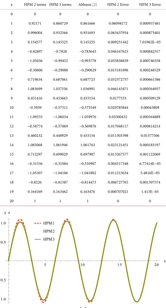
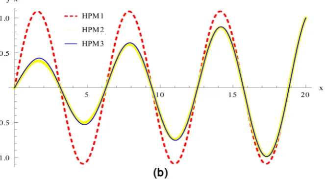
From Table 1, Figure 1(a) and Figure 1(b), it can be seen that there is an in-significant difference between the results of two and three terms HPM solutions and exact solution. It motivates us to move onto the next studies using different boundary conditions.
Example 2: Consider the VDP equation with first Robin type boundary con-dition
(
2 1)
0,( )
0 0,( )
20 1y u y′′+ − y y′+ = y = y′ =
The Homotopy is,
(
0 0) (
0 0)
(
2 1)
0Y Y′′+ − y′′+y +t y′′−y +t u Y − Y′=
Putting,
[ ] [ ]
2
0 1 2, 0 sec 20 sin
Y Y tY t Y y= + + = x ,
in Equation (3.1) and equating the coefficients of t from both sides, we get
( )
( )
0 0 0
0 0, 0 0, 20 1
y′′+y = y = y′ =
( )
( )
2
0 1
1 1 0 0 0, 1 0 0, 20 0
y y uy y uy′′+ + ′− ′= y = y′ =
( )
( )
2
2 0 1 0 1 2 2
2 2 0 1 0, 0 0, 20 0
DOI: 10.4236/jamp.2019.71001 5 Journal of Applied Mathematics and Physics
Table 1. Relative errors for example 1 (Using u=0.01).
x HPM 2 terms HPM 3 terms Abbassi [2] HPM 2 Error HPM 3 Error
0 0 0 0 0 0
1 0.92171 0.860729 0.861666 0.06098172 0.000937481 2 0.996004 0.932566 0.931693 0.063437934 0.000873401 3 0.154577 0.145325 0.145255 0.009251442 7.01962E−05 4 −0.82897 −0.7828 −0.783643 0.046167623 0.000842517 5 −1.05036 −0.99452 −0.993778 0.055838839 0.000746558 6 −0.30606 −0.29088 −0.290629 0.015181896 0.000248529 7 0.719634 0.687061 0.687723 0.032572757 0.000661586 8 1.083699 1.037556 1.036991 0.046143471 0.000564957 9 0.451416 0.433663 0.433154 0.0177533 0.000509129 10 −0.5959 −0.57511 −0.575549 0.020785844 0.00043809 11 −1.09535 −1.06034 −1.059976 0.03500432 0.000364889 12 −0.58774 −0.57069 −0.569876 0.017048117 0.000814214 13 0.460232 0.448929 0.433154 0.011303398 0.01577506 14 1.085068 1.061946 1.061763 0.023121451 0.000183197 15 0.712297 0.699029 0.697907 0.013267577 0.001122069 16 −0.31536 −0.31084 −0.310907 0.004517348 6.77414E−05 17 −1.05307 −1.04186 −1.041802 0.011215634 5.4816E−05 18 −0.8226 −0.81587 −0.814473 0.006727765 0.001397574 19 0.164169 0.163462 0.163476 0.000707021 1.413E−05
DOI: 10.4236/jamp.2019.71001 6 Journal of Applied Mathematics and Physics
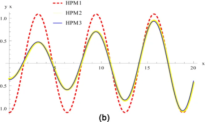
Figure 1. (a) Approximate solutions using u = 0.01; (b) Approximate solutions using u = 0.1.
Solving we get,
[ ] [ ]
0 sec 20 sin
y = x
[ ]
[ ]
(
(
[ ]
)
[ ] [ ]
[ ] [ ]
[ ] [ ]
[ ]
)
3
1 321 sec 20 sin 160 4 8cos 40 80cos 60 sec 20
7sec 20 sin 60 4cos sin tan 20
y u x x
x x
= − + + −
− + +
[ ]
(
[ ]
[ ]
[ ]
(
[ ]
[ ]
)
[ ]
[ ]
(
)
[ ]
(
[ ]
)
[ ]
[ ]
[ ]
[ ]
(
[ ]
[ ]
[ ] [ ] [ ]
[ ]
)
6 2
2
4
3 5
7 2
2 4
1
sec 20 5 100cos sin
6144
2cos 118 72cos 40 25cos 2 sin
36 48cos 80 sin 6 3 8cos 40 sin
20sin 12cos sin 17 8cos 40
4cos 80 4cos 60 sec 20 sin 15sin
y u x x
x x x
x x
x x x
x x
= − −
− − + +
+ − + +
− + − +
− − +
(
)
[ ] [ ]
[ ]
(
[ ]
(
)
[ ] [ ]
[ ] [ ]
[ ]
)
[ ]
(
(
[ ]
)
[ ] [ ]
[ ] [ ]
[ ] [ ]
[ ] [ ]
3 5
2
36 20 csc sin 2 18cos 160
4 8cos 40 80cos 60 sec 20 7sec 20 sin 60
tan 20 sin 19431 48 1 2cos 80 19356cos 60 sec 20 18838cos 100 sec 20 73cos 140 sec 20 3840sec 20 sin 60
x x x x
x
x x
+ − + − −
+ + − −
+ − + +
+ +
+ −
[ ] [ ]
[ ]
(
[ ]
[ ]
[ ]
[ ]
[ ]
[ ]
)
[ ]
[ ]
[ ]
[ ] [ ] [ ]
[ ] [ ] [ ]
[ ] [ ] [ ]
[ ] [ ] [ ]
2
3360sec 20 sin 100 24 sec 20 80cos 20 80cos 60 80cos 100 9sin 20 8sin 60
7sin 100 9120sin 2 81sin 2 960 tan 20 1920cos 60 sec 20 tan 20 960cos 100 sec 20 tan 20 576sec 20 sin 60 tan 20 220sec 20 sin 100 tan 20
x
x x
+ −
+ + + −
+ − + +
− −
DOI: 10.4236/jamp.2019.71001 7 Journal of Applied Mathematics and Physics
[ ] [ ] [ ]
[ ]
)
[ ]
(
[ ]
(
[ ]
[ ]
[ ]
[ ]
)
[ ]
(
[ ]
)
(
(
[ ]
)
[ ] [ ]
[ ] [ ]
[ ]
)
)
[ ]
(
[ ]
(
[ ]
[ ]
2 3 273sec 20 sin 140 tan 20 429 tan 20
12cos 3sec 20 80cos 60 4 cos 60 sin 20 7sin 60 sin 2 2 cos 40 160 4 8cos 40 80cos 60 sec 20 7sec 20 sin 60 tan 20
6cos sec 20 320cos 20 80cos 60
x x x x x + + + − + + − − − + − + + − − + + +
[ ]
(
[ ]
[ ]
[ ]
)
[ ]
[ ]
[ ]
)
[ ]
(
[ ]
[ ]
(
[ ]
160cos 100 4 3cos 20 3cos 60 4cos 100 21sin 20 37sin 60 14sin 100
2sec 20 800cos 60 80cos 100 4 19cos 20 x x − + + + − + − − − − +
[ ]
[ ]
)
[ ]
[ ]
)
[ ]
[ ]
(
(
[ ]
)
[ ] [ ]
[ ] [ ]
[ ]
)))
2 410cos 60 cos 100 55sin 60 7sin 100 sin 9sin 160 4 8cos 40 80cos 60 sec 20 7sec 20 sin 60 tan 20
x
x x
+ + − −
+ − + + −
− +
Example 3: Consider the VDP equation with second Robin type boundary condition
(
2 1)
0,( )
0 0,( )
20 1y u y′′+ − y y′+ = y′ = y =
The Homotopy is,
(
0 0) (
0 0)
(
2 1)
0Y Y′′+ − y′′+y +t y′′−y +t u Y − Y′=
Putting,
[ ] [ ]
2
0 1 2, 0 cos sec 20
Y Y tY t Y y= + + = x ,
in Equation (3.1) and equating the coefficients of t from both sides, we get
( )
( )
0 0 0
0 0, 0 0, 20 1
y′′+y = y′ = y =
( )
( )
2
1 0 0 1 1
1 0 0, 0 0, 20 0
y y u y y uy′′+ + ′− ′= y′ = y =
( )
( )
2
2 0 1 0 1 0 1 2 2
2 2 0, 0 0, 20 0
y′′+y + uy y y uy uy y′− ′+ ′= y′ = y =
Solving we get,
[ ] [ ]
0 cos sec 20
y = x
[ ]
(
[ ]
[ ]
[ ]
(
[ ]
[ ]
)
[ ]
(
(
[ ]
)
[ ] [ ]
[ ] [ ]
[ ]
))
3 2 1 21 sec 20 7cos sin sin 1 16cos 40 64
sin 2cos 160 4 8cos 40
80cos 60 sec 20 5sec 20 sin 60 3tan 20
y u x x x
x x x
= − + − − + + − + + − + −
[ ]
(
[ ]
[ ]
(
[ ]
[ ]
)
[ ]
(
[ ]
[ ]
[ ]
(
)
[ ]
[ ]
)
[ ]
[ ]
(
[ ]
(
[ ]
[ ]
[ ]
[ ]
[ ]
)
[ ]
5 7 5
2 2 3 2 4 2 2
1 sec 20 20cos 6cos 18 16cos 40
6144
15cos 2 4cos 33 96cos 40 12cos 80 69 48cos 40 sin 25sin
12cos sin 3sec 20 160cos 20 80cos 60 4 cos 60 3sin 20 5sin 60 sin
y u x x
DOI: 10.4236/jamp.2019.71001 8 Journal of Applied Mathematics and Physics
[ ]
(
)
(
(
[ ]
)
[ ] [ ]
[ ] [ ]
[ ]
)
)
[ ]
[ ]
(
(
[ ]
)
[ ] [ ]
[ ] [ ]
[ ]
)
[ ]
(
[ ] [ ]
42 4 cos 40 160 4 8cos 40
80cos 60 sec 20 5sec 20 sin 60 3tan 20 54cos sin 160 4 8cos 40 80cos 60 sec 20 5sec 20 sin 60 3tan 20 6sin 1280 36 560cos 60 sec 20
x
x x x
x x − + − + + − + − + − + + − + − − + +
[ ] [ ]
[ ] [ ]
[ ] [ ]
[ ] [ ]
[ ]
[ ]
(
)
[ ]
(
(
[ ]
)
[ ] [ ]
[ ] [ ]
[ ]
)
[ ]
(
(
[ ]
)
[ ] [ ]
2 2 420 cos 60 sec 20 160cos 100 sec 20
61sec 20 sin 60 10sec 20 sin 100 12 sin 2 4 2 cos 40 sin 160 4 8cos 40 80cos 60 sec 20 5sec 20 sin 60 3tan 20 3sin 160 4 8cos 40 80cos 60 sec 20
x x x x x x x + − − + − + − + − + + − + − + − + + −
[ ] [ ]
[ ]
)
[ ]
)
[ ]
(
(
[ ]
)
[ ] [ ]
[ ] [ ]
[ ] [ ]
[ ] [ ]
[ ]
(
[ ]
[ ]
[ ]
[ ]
[ ]
[ ]
)
25sec 20 sin 60 3tan 20 49 tan 20
cos 19455 48 1 2cos 80 19404cos 60 sec 20 19214cos 100 sec 20 7cos 140 sec 20
3840sec 20 sin 60 24 sec 20 80cos 20 80cos 60 80cos 100 11sin 20 8sin 60 5sin 100
x x x + − + + + + + + − + − + + − + −
[ ] [ ]
(
[ ]
[ ]
)
[ ]
[ ]
(
)
[ ]
[ ]
[ ]
[ ] [ ] [ ]
[ ] [ ] [ ]
[ ] [ ] [ ]
[ ] [ ] [ ]
[ ] [ ] [ ]
[ ]
)
)
2 4 6 22400sec 20 sin 100 12 9 56cos 40 4cos 80 sin 6 31 48cos 40 sin 100sin 6720 tan 20 5760cos 60 sec 20 tan 20 960cos 100 sec 20 tan 20 576sec 20 sin 60 tan 20 92sec 20 sin 100 tan 20 7sec 20 sin 140 tan 20 477 tan 20
x x x − + + − − + + + + − − + − +
Example 4: Consider the VDP equation with Neumann type boundary condi-tion
(
2 1)
0,( )
0 0,( )
20 1y u y′′+ − y y′+ = y′ = y′ =
The Homotopy is,
(
0 0) (
0 0)
(
2 1)
0Y Y′′+ − y′′+y +t y′′−y +t u Y − Y′=
Putting,
[ ] [ ]
2
0 1 2, 0 cos csc 20
Y Y tY t Y y= + + = − x ,
in Equation (3.1) and equating the coefficients of t from both sides, we get
( )
( )
0 0 0, 0 0 0, 0 20 1
y′′+y = y′ = y′ =
( )
( )
2
1 1 0 0 0 0, 1 0 0, 1 20 0
y y uy y uy′′+ + ′− ′= y′ = y′ =
( )
( )
2
2 2 2 0 1 0 1 0 1 0, 2 0 0, 2 20 0
y′′+y + uy y y uy uy y′− ′+ ′= y′ = y′ =
DOI: 10.4236/jamp.2019.71001 9 Journal of Applied Mathematics and Physics
[ ] [ ]
0 cos csc 20
y = − x
[ ]
(
[ ]
(
[ ]
(
[ ]
)
[ ]
)
[ ]
[ ]
[ ]
(
[ ]
[ ]
)
)
3 1
2 2
1 csc 20 2cos 40 80cos 40 2 4cos 40 3sin 40 32
3cos sin sin 1 8cos 40 sin
y u x x
x x x x
= − + − + −
+ − − + +
[ ]
(
[ ]
[ ]
(
[ ]
[ ]
(
)
[ ]
)
[ ]
[ ]
(
[ ]
[ ]
)
[ ]
(
[ ]
[ ]
[ ]
[ ]
(
)
[ ]
(
[ ]
)
[ ]
(
)
[ ]
)
5 5 2
2 2
3
2
2
1 csc 20 30cos 63cos 40 80cos 40 3072
2 4cos 40 3sin 40 sin cos 1 84cos 40 25sin 3sin 520 1680cos 40 640cos 80 2 9 14cos 40 8cos 80 87sin[40] 24sin[80] 3 40 80cos 40 2 4cos 40 3sin 40 sin
y u x x
x x x
x x
x
x x
= − −
+ − + − − +
+ + − −
+ − + − −
+ − + − + −
[ ]
(
[ ]
(
[ ]
[ ]
[ ]
[ ]
[ ]
[ ]
[ ]
[ ]
[ ]
(
)
(
[ ]
[ ]
(
[ ]
[ ]
[ ]
)
)
)
[ ]
(
)
[ ]
[ ]
)
)
2
2 4
cos csc 20 1440cos 20 3840cos 60
240cos 100 9540sin 20 9399sin 60 9430sin 100 24 sin 20 sin 60 sin 100 12 3cos 20 3cos 100 80 sin 20 sin 60 sin 100
36 2 7cos 40 sin 25sin
x
x x
x x
+ − +
− + − +
+ − + + −
+ − − +
+ − + +
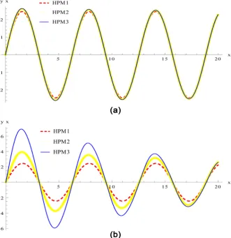
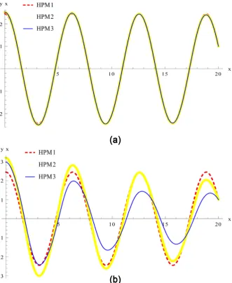
[image:9.595.208.540.360.702.2]From Figures 2-4 it can be seen that VDPDE with different boundary
DOI: 10.4236/jamp.2019.71001 10 Journal of Applied Mathematics and Physics
DOI: 10.4236/jamp.2019.71001 11 Journal of Applied Mathematics and Physics
Figure 4. (a) Approximate solutions using u = 0.01; (b) Approximate solutions using u = 0.1.
conditions can be solved by HPM very easily. Two terms and three terms solu-tion almost coincide. Increasing the number of terms, more accurate results can be found. The solution can be obtained by using different values of u.
4. Conclusion
In this research, HPM is applied for the solution of the Van Der Pol differential equation with different boundary conditions. One, two and three parameters HP solutions are developed and presented graphically. It is found that higher para-meter shows good approximations of the analytical solution. It may conclude that HPM is a very effective technique to find the analytical solutions for highly non-linear ordinary differential equation with ICs/BCs.
Conflicts of Interest
The author declares no conflicts of interest regarding the publication of this pa-per.
References
[1] Buonomo, A. (1998) The Periodic Solution of Van der Pol’s Equation. SIAM Jour-nal of Applied Mathematics, 59, 156-171.
https://doi.org/10.1137/S0036139997319797
[2] Abbasi, N.M. (2009) Solving the Van Der Pol Nonlinear Differential Equation Us-ing First Order Approximation Perturbation Method.
[3] Deeba, E. and Xie, S. (2001) The Asymptotic Expansion and Numerical Verification of Van der Pol’s Equation. Journal of Computational Analysis and Applications, 3, 165-171.https://doi.org/10.1023/A:1010189225921
[4] He, J.H. (1999) Homotopy Perturbation Technique. Computer Methods in Applied Mechanics and Engineering, 178, 257-262.
https://doi.org/10.1016/S0045-7825(99)00018-3
Me-DOI: 10.4236/jamp.2019.71001 12 Journal of Applied Mathematics and Physics thod. Computers and Mathematics with Applications, 57, 410-412.
https://doi.org/10.1016/j.camwa.2008.06.003
[6] Rafiq, A., Ahmed, M. and Hussain, S. (2008) A General Approach to Specific Second Order Ordinary Differential Equations Using Homotopy Perturbation Me-thod. Physics Letters A,372, 4973-4976.
https://doi.org/10.1016/j.physleta.2008.05.070
[7] Chowdhury, M.S.H. and Hashim, I. (2009) Solutions of Emden-Fowler Equations by Homotopy Perturbation Method. Nonlinear Analysis: Real World Applications, 10, 104-115.https://doi.org/10.1016/j.nonrwa.2007.08.017
[8] Yıldırım, A. and Özis, T. (2007) Solutions of Singular IVPs of Lane-Emden Type by Homotopy Perturbation Method. Physics Letters A, 369, 70-76.
https://doi.org/10.1016/j.physleta.2007.04.072
[9] Saadatmandia, A., Dehghanb, M. and Eftekharia, A. (2009) Application of He’s Homotopy Perturbation Method for Non-Linear System of Second-Order Boun-dary Value Problems. Nonlinear Analysis: Real World Applications,10, 1912-1922.