Statistical Analysis of Process Monitoring Data for Software Process Improvement and Its Application

Statistical Analysis of Process Monitoring Data for

Software Process Improvement and Its Application

Kazuhiro Esaki1, Yuki Ichinose2, Shigeru Yamada2 1

Fuculty of Science and Engineering, Hosei University, Tokyo, Japan

2

Graduate School of Engineering, Tottori University, Tottori, Japan

Email: [email protected], [email protected], [email protected]

Received November 28, 2011; revised December 29, 2011; accepted January 14, 2012

ABSTRACT

Software projects influenced by many human factors generate various risks. In order to develop highly quality software, it is important to respond to these risks reasonably and promptly. In addition, it is not easy for project managers to deal with these risks completely. Therefore, it is essential to manage the process quality by promoting activities of process monitoring and design quality assessment. In this paper, we discuss statistical data analysis for actual project manage-ment activities in process monitoring and design quality assessmanage-ment, and analyze the effects for these software process improvement quantitatively by applying the methods of multivariate analysis. Then, we show how process factors affect the management measures of QCD (Quality, Cost, Delivery) by applying the multiple regression analyses to observed process monitoring data. Further, we quantitatively evaluate the effect by performing design quality assessment based on the principal component analysis and the factor analysis. As a result of analysis, we show that the design quality as-sessment activities are so effective for software process improvement. Further, based on the result of quantitative pro-ject assessment, we discuss the usefulness of process monitoring progress assessment by using a software reliability growth model. This result may enable us to give a useful quantitative measure of product release determination.

Keywords: Software Process Improvement; Process Monitoring; Design Quality Assessment; Multiple Regression Analysis; Principal Component Analysis; Factor Analysis; Quantitative Project Assessment

1. Introduction

In recent years, with dependence of the computerized system, software development has become more large- scaled, complicated, and diversified. At the same time, customer’s demand of high quality and shortened deliv-ery has increased. Therefore, we have to pursue the pro-ject management efficiently in order to develop highly quality software products. Also, we need to statistically analyze process data observed in software development projects. Based on the process data, we can establish the PDCA (Plan-Do-Check-Act) management cycle in order to improve the software development process with respect to software management measures about QCD (Quality, Cost, Delivery) [1,2].

There are many risks latent in promoting software pro-jects. These risks often lead to QCD (Quality, Cost, De-livery) related problems, such as system failures, budget overruns, and delivery delays which may cause the pro-ject to fail. In order to lead a software propro-ject to become successful, project managers need to conduct adequate project management techniques in the software develop-ment process with technological and managedevelop-ment skills.

However, it is not easy for them to respond to all the risks. Therefore, we discuss the following two improve-ment activities:

 Process monitoring activities;

 Assessment activities of design quality.

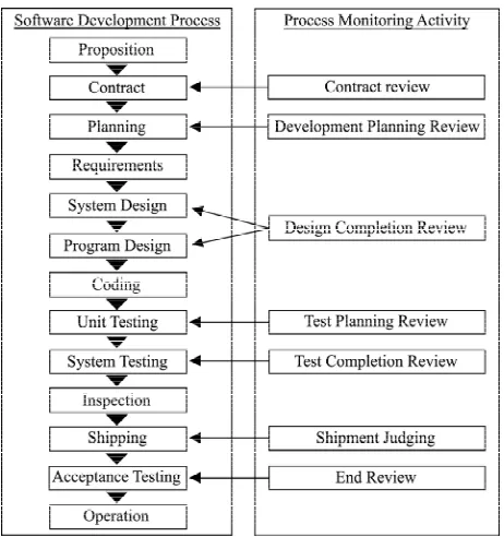
Process monitoring activities review the process from the early-stage of the project by a third person of the quality assurance unit to find latent project risks and QCD related problems as shown in Figure 1 [3]. The process monitoring activity may help project managers to pursue the project management efficiently and also im-prove management process to lead a project to success. Assessment activities of design quality evaluate the com-pleteness of required specifications and design specifica-tions by third person as well as process monitoring ac-tivities. The assessment activities of design quality may improve the software development process by eliminat-ing software faults.

Figure 1.Overviews of the process monitoring activities.

analysis. At the same time, we use collaborative filtering to estimate of the missing value. Based on the derived quality prediction models, we make the software process factors affecting quality of software product clear. Sec-tion 3 evaluates the effect quantitatively by introducing design quality assessment activities into process moni-toring based on the principal component analysis and the factor analysis. Further, Section 4 discusses a method of quantitative project assessment with the process moni-toring data based on a software reliability growth model. Finally, Section 5 summarizes the results obtained in this paper.

2. Factorial Analysis Affecting the Software

Quality

2.1. Process Monitoring Data

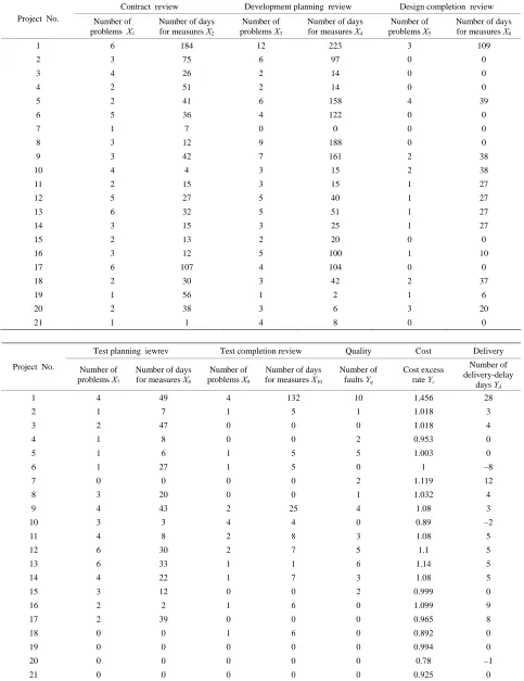
We analyze the factors affecting the quality of software products by using the process monitoring data as shown in Table 1. Ten variables measured by the process moni-toring are used as explanatory variables. Three variables such as software management measures of QCD are used as objective variables. These variables are defined in the following:

X1: The number of problems detected in the contract review.

X2: The number of days how long it took for the prob-lems to be solved in the contract review.

X3: The number of problems detected in the develop-ment planning review.

X4: The number of days how long it took for the

prob-lems to be solved in the development planning review.

X5: The number of problems detected in the design completion review.

X6: The number of days how long it took for the prob-lems to be solved in the design completion review.

X7: The number of problems detected in the test plan-ning review.

X8: The number of days how long it took for the prob-lems to be solved in the test planning review.

X9: The number of problems detected in the test com-pletion review.

X10: The number of days how long it took for the prob-lems to be solved in the test completion review.

Yq: The number of detected faults given by the

fol-lowing expressions:

(The number of faults) = (The number of faults de-tected during acceptance testing) + (The number of faults detected during production).

Yc: The cost excess rate given by the following

expres-sions:

(Cost excess rate) = (Actual cost value)/(Scheduled software development cost).

If the cost excesses rate is over 1.0, it means that the expenses exceed the software development budget.

Yd: The number of delivery-delay days to the shipping

time planned at the project initiation time.

There are some missing values in Table 1. Therefore, we apply collaborative filtering [6] to estimate of these missing values. And projectNo.17-projectNo.21 are ones in which design quality assessment was carried out, whereas projectNo.1-projectNo.16 are ones in which design quality assessment was not assessed.

2.2. Multiple Regression Analysis

By using the process monitoring data in Table 1, we can perform correlation analysis among the explanatory and objective variables as follows:

 Contract review, design completion review, and test completion review have shown strong correlations to the measures of QCD.

 Yq has shown strong correlation to Yc and Yd.

Based on the correlation analysis, we can find that it is important to reduce the number of faults and ensure the software quality in order to prevent cost excess and de-livery-delay. Therefore, X5, X7, and X10 are selected as important factors for estimating a software quality pre-diction model [7,8].

Then, a multiple regression analysis is applied to the process monitoring data as shown in Table 1. Then, us-ing X5, X7, and X10, we have the estimated multiple re-gression equation predicting for software faults, , given by Equation (1) as well as the normalized multiple regression expression,

ˆ

q

Y

ˆN q

Table 1. Observed process monitoring data.

Contract review Development planning review Design completion review Project .No _{Number of}

problems X1

Number of days for measures X2

Number of problems X3

Number of days for measures X4

Number of problems X5

Number of days for measures X6

1 6 184 12 223 3 109 2 3 75 6 97 0 0 3 4 26 2 14 0 0 4 2 51 2 14 0 0 5 2 41 6 158 4 39 6 5 36 4 122 0 0 7 1 7 0 0 0 0 8 3 12 9 188 0 0 9 3 42 7 161 2 38 10 4 4 3 15 2 38 11 2 15 3 15 1 27 12 5 27 5 40 1 27 13 6 32 5 51 1 27 14 3 15 3 25 1 27 15 2 13 2 20 0 0 16 3 12 5 100 1 10 17 6 107 4 104 0 0 18 2 30 3 42 2 37 19 1 56 1 2 1 6 20 2 38 3 6 3 20 21 1 1 4 8 0 0

Test planning iewrev Test completion review Quality Cost Delivery

Project .No _{Number of} problems X7

Number of days for measures X8

Number of problems X9

Number of days for measures X10

Number of faults Yq

Cost excess rate Yc

Number of delivery-delay

days Yd

1 4 49 4 132 10 1.456 28

2 1 7 1 5 1 1.018 3

3 2 47 0 0 0 1.018 4

4 1 8 0 0 2 0.953 0

5 1 6 1 5 5 1.003 0

6 1 27 1 5 0 1 –8

7 0 0 0 0 2 1.119 12

8 3 20 0 0 1 1.032 4

9 4 43 2 25 4 1.08 3

10 3 3 4 4 0 0.89 –2

11 4 8 2 8 3 1.08 5

12 6 30 2 7 5 1.1 5

13 6 33 1 1 6 1.14 5

14 4 22 1 7 3 1.08 5

15 3 12 0 0 2 0.999 0

16 2 2 1 6 0 1.099 9

17 2 39 0 0 0 0.965 8

18 0 0 1 6 0 0.892 0

19 0 0 0 0 0 0.994 0

20 0 0 0 0 0 0.78 –1

21 0 0 0 0 0 0.925 0

5 7 10

ˆ _{0.661 0.540 0.043 0.024,}

q

Y  X  X  X  (1)

5 7

ˆN _{0.292 0.354 0.501 .}

q

Y  X  X  X10



i

(2)

In order to check the goodness-of-fit adequacy of our model, the coefficient of multiple determination R2 is calculated as 0.735. Furthermore, the squared multiple correlation coefficient adjusted for degrees of freedom (adjusted R2), called the contribution ratio, is given by 0.669. The result of multiple regression analysis is sum-marized in Tables 2-3.

From Table 2, it is found that the precision of these multiple regression equations is high. Then, we can pre-dict the number of faults detected for the final products by using Equation (1). From Equation (2), the order of the degree affecting the objective variable Yq is X5 < X7 <

X10. Therefore, we conclude that the design completion review, the test planning review, and the test completion review have an important impact on product quality.

3. Analysis of the Effect of Design Quality

Assessment

3.1. Analysis Data

We analyze the effect of design quality assessment by using the process monitoring data in Table 1. Then, we assume that the model signifies that although the risks at the start of the project negatively affect the management measures of QCD, the QCD can be improved by process monitoring activities and design quality assessment. Based on this hypothetical model, we analyze by using initial project risks data (as shown in Table 4) as well as the process monitoring data. These new variables are explained in the following:

X11: The risk ratio of project initiation. The risk ratio is given by the following expressions:

 

 



i

R



Table 2. Table of analysis of variance.

Source of variation DF SSq MSq F-value

Due to regression 3 83.050 27.683 11.0920**

Error 12 29.950 2.496

Total 15 113.000

**

means statistical significance at 1% level.

Table 3. Estimated parameters.

Factor Coefficient SE t-value Standard coefficient

Intercept 0.024 0.784 0.030

X5 0.661 0.393 1.680 0.292

X7 0.540 0.235 2.302 0.354

X10 0.043

Table 4. Initial project risks data.

0.015 2.879 0.501

Project No.

Risk ratio (0 ~ 100) X11

Development si ze )(ksteps

X12

Development period )(days

X13

Estimated man-hours

) H ( X14

1 45 10.2 41 931

2 19 9.3 66 955

3 13 5.8 53 606

4 11 11.8 91 997

5 24 13.3 152 1590

6 17 26.8 122 2629

7 17 1.4 24 187

8 29 4.7 47 389

9 35 8.3 67 749

10 25 28.9 138 2392

11 28 26.2 91 3872

12 38 12.4 91 1729

13 42 13.7 91 2088

14 30 7.8 91 1191

15 28 6.7 71 695

16 35 1.6 28 268

17 23 13.6 56 687

18 29 2.9 73 595

19 25 21.4 121 1519

20 18 0.6 84 694

21 30 8.5 115 2275

where the risk estimation checklist has weight (i) in each risk item (i), and the risk score ranges between 0 and 100 points. Project risks are identified by interviewing using the risk estimation checklist. From the identified risks, the risk score of a project is calculated by Equation (3).

X12: The development size. The development size is given by the following expressions: Development size (Kilo (103) steps) = (Number of newly developed steps) + 1.5 × (Number of modified steps) + (Influential rate) × (Number of reused steps). The influential rate ranges between 0.01 and 0.1.

X13: The number of days during development period.

X14: The estimated man-hours (the development budg-ets divided by the development cost per hour).

3.2. Principal Component Analysis

4. It is found that the precision of analysis is high from Ta- ble 5. And the factor loading values are obtained as shown in Table 6. The principal component scores are obtained as shown in Table 7. From Table 6, let us newly define the first and second principal components as follows:  The first principal component is defined as the

meas-ure for QCD attainment levels.

 The second principal component is defined as the measure for software project estimation (development size, period, effort).

We obtain a scatter plot of the factor loading values in Figure 2. From Figure 2, it is found that the factors of process monitoring have shown positive correlation to the management measures of QCD. Therefore, we can consider that the process monitoring activities have an important impact on the management measures of QCD.

Further, we also obtain a scatter plot of the principal component scores as shown in Figure 3. Projects in which design quality assessment was carried out are in-dicated by the “” marks, whereas “” marks indicate

Table 5. Summary of eigenvalues and principal compo-nents.

Component Eigenvalue Contribution ratio

Cumulative contribution ratio

1 7.625 0.449 0.449

2 3.047 0.179 0.628

Table 6. Factor loading values.

Component 1 Component 2

X1 0.632 0.112

X2 0.700 –0.169

X3 0.815 –0.069

X4 0.694 –0.153

X5 0.430 0.309

X6 0.844 0.240

X7 0.609 0.260

X8 0.654 –0.116

X9 0.692 0.505

X10 0.891 –0.069

X11 0.719 0.123

X12 0.021 0.857

X13 –0.261 0.854

X14 –0.021 0.888

Yq 0.850 0.113

Yc 0.843 –0.155

Yd 0.722

Table 7. Principal component scores.

Component 1 Component 2

1 3.673 –0.478

2 0.205– 0.588–

3 0.459– 0.974–

4 0.827– 0.256–

5 0.177 1.021

6 0.426– 1.231

7 0.712– 1.640–

8 0.096 –1.133

9 0.904 –0.143

10 0.225– 2.257

11 0.003– 1.674

12 0.680 0.660

13 0.788 0.702

14 0.074 0.074

15 0.566– 0.500–

16 0.047 1.203–

17 0.094 0.803–

18 0.461– 0.367–

19 0.862– 0.556

20 0.850– 0.392–

21 0.938– 0.300

Figure 2. Scatter plot of the factor loading values.

–0.422

Figure 3. Scatter plot of the principal component scores.

3.3. Factor Analysis

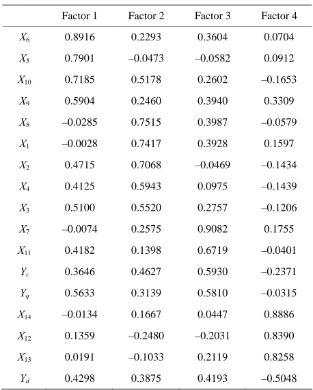
Factor analysis is performed by using the process moni-toring data and initial project risks data in Tables 1 and 4 as well as principal component analysis. Then, the method of varimax rotation is applied to the rotation of factor axes. From Table 8, it is found that the precision of analysis is high. And the factor loading values are ob-tained as shown in Table 9. The factor scores are ob-tained as shown in Table 10.

From Table 9, it is found that X5, X6, X9, and X10 are the same group factors considered as “the value of pro-ject attainment”, X1, X2, X3, X4, and X8 as “the value of project planning”, X7, X11, Yq, and Yc as “the value of

quality and cost”, and X12, X13, X14, and Yd as “the value

of estimation and delivery”.

From Table 10, it is found that the values of the third factor of all the projects in which the design quality as-sessment activities were carried out are small. This result has shown that the projects in which the design quality assessment activities were carried out can reduce the number of faults, the cost excess, and the delivery-delay.

4. Quantitative Project Assessment

Next, we discuss quantitative project assessment based on the process monitoring data. A project progress growth curve in the process monitoring activities is assumed to be the relationship between the number of process moni-toring progress phases and the cumulative number of QCD problems detected during the process monitoring. Then, we apply Moranda geometric Poisson model [9], which is a software reliability growth model (SRGM), to the process monitoring data on X1, X3, X5, X7, and X9 as shown in Table 1.

We discuss project progress modeling based on the Moranda geometric Poisson model because an analytic treatment of it is relatively easy. Then, we choose the number of process monitoring progress phases as the alternative unit of testing-time by assuming that the ob-served data for testing-time are discrete in an SRGM.

In order to describe a fault-detection phenomenon dur-

Table 8. Analysis precision.

No. SSq Contribution ratio Cumulative contribution ratio

Factor 1 3.77 0.222 0.222

Factor 2 3.30 0.194 0.416

Factor 3 2.99 0.176 0.592

Factor 4 2.75 0.162 0.754

Table 9. Factor loading values.

Factor 1 Factor 2 Factor 3 Factor 4 X6 0.8916 0.2293 0.3604 0.0704

X5 0.7901 –0.0473 –0.0582 0.0912

X10 0.7185 0.5178 0.2602 –0.1653

X9 0.5904 0.2460 0.3940 0.3309

X8 –0.0285 0.7515 0.3987 –0.0579

X1 –0.0028 0.7417 0.3928 0.1597

X2 0.4715 0.7068 –0.0469 –0.1434

X4 0.4125 0.5943 0.0975 –0.1439

X3 0.5100 0.5520 0.2757 –0.1206

X7 –0.0074 0.2575 0.9082 0.1755

X11 0.4182 0.1398 0.6719 –0.0401

Yc 0.3646 0.4627 0.5930 –0.2371 Yq 0.5633 0.3139 0.5810 –0.0315 X14 –0.0134 0.1667 0.0447 0.8886

X12 0.1359 –0.2480 –0.2031 0.8390

X13 0.0191 –0.1033 0.2119 0.8258

Yd 0.4298 0.3875 0.4193 –0.5048

ing processing monitoring progress phase i (i1, 2,), let Ni denote a random variable representing the number

of problems detected during ith project monitoring pro-gress interval (Ti–1, Ti] (T0 = 0; ). Then, the problem-detection phenomenon can be described as fol-lows:

1, 2,

i 













1

1

Pr exp

!

0, 0 1; 0,1, 2, ,

n i

i i

k

N n k

n

k n













  _

    

 (4)

where Pr{A} means the probability of event A, and  = the average number of problems detected in the first interval (0, T1],

k = the decrease ratio of the number of problems de-tected by process monitoring activities.

From Equation (4), setting Ti = i (i ), we

ob-tain the following quantitative project assessment meas-ures, that is, the expected cumulative number of prob-lems detected up to nth process monitoring progress

1, 2,

Table 10. Factor scores.

Factor 1 Factor 2 Factor 3 Factor 4

1 3.0741 2.2501 0.9193 –0.7904

2 –0.7503 0.6891 –0.9300 –0.5207

3 –1.1537 0.8149 –0.3592 –0.5439

4 –0.1758 –0.2290 –0.6508 0.0725

5 1.5491 –0.6982 –0.6785 0.8107

6 –0.7755 1.2644 –0.9234 1.6292

7 –0.4762 –0.7392 –0.7101 –1.7617

8 0.0733 0.2048 0.3177 –0.6335

9 –0.1981 0.8603 0.0369 –0.4353

10 0.3662 –0.2572 –0.2913 2.1230

11 0.0939 –1.0389 1.5943 1.3390

12 –0.4992 0.1541 1.6362 0.4280

13 –0.3883 0.5109 1.2508 0.5704

14 0.3214 –1.4278 2.0740 –0.0154

15 –1.0662 –0.5627 0.8184 –0.5421

16 –0.6646 –0.3412 0.6625 –1.4622

17 –1.2274 1.5995 –0.4419 –0.2308

18 2.0095 –1.5983 –0.7339 –0.4427

19 0.0942 –0.1969 –1.2528 0.8626

20 0.1174 –0.4808 –1.3677 –0.5964

21 –0.3238 –0.7776 –0.9705 0.1397

phase, E(n), and the expected total number of problems latent in the software project, , are given as Equa-tions (5) and (6), respectively:

 

 

_



_



1

1 , 1

n n

i i

k

E n k

k    



 





 

 

1

n

E E n

k

 

  

 (6)

Project assessment measures play an important role in quantitative assessment of process monitoring progress. The expected number of remaining problems, r(n), represents the number of problems latent in the software project at the end of nth process monitoring progress phase, and is formulated as

 

 

 

r n E  E n , (7)

and the instantaneous MTBP which means mean time between problem occurrences is formulated as

 

1 MTBP n _n ,

k

 

 (8)

Further, a project reliability represents the probability

that a problem dose not occur in the time-interval (n, n + 1] (n ≥ 0) given that the process monitoring progress has been going up to phase n. Then, the project reliability function is derived as

 

exp n

R n  _k  _. (9)

We present numerical examples by using the Moranda geometric Poisson model for ProjectNo.5. Figure 4 shows the estimated cumulative number of problems detected,

E(n), and the actual measured values during process monitoring progress interval (0, n] where the estimated parameters are given as ˆ = 4.39 and = 0.773 by using a method of maximum-likelihood. Figure 5 shows the estimated expected number of remaining problems,

r(n). From Figure 5, it is found that there are 5 problems remaining at the end of test completion review phase (n = 5).

ˆ

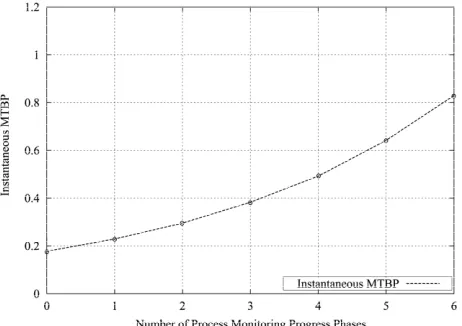
k

Further, the estimated instantaneous MTBP is obtained as shown in Figure 6. From Figure 6, it is found that the process monitoring activities is going well because the MTBP is growing. As for project reliability, it is neces-sary to keep conducting the process monitoring activities because the project reliability after the test completion review is 39 percent.

5. Concluding Remarks

In this paper, we have discussed statistical data analysis for actual activities for process monitoring and design quality assessment, and analyzed these effects for soft-ware process improvement quantitatively by applying the methods of multivariate analysis. We have found how process factors affect the management measures of QCD by applying the multiple regression analyses to observed process monitoring data. Further, we have evaluated the effect quantitatively by performing design quality as-sessment based on the principal component analysis and

Figure 5. The estimated expected number of remaining problems, r(n).

Figure 6. The estimated instaneous MTBP, MTBP(n).

multiple regression analysis, we have found that the de-sign completion review, the test planning review, and the test completion review have an impact on final product quality. Then, we can consider that the problems in the test planning review and the test completion review were influenced by those in the design completion review. That is, it is very important to manage the design quality in soft- ware development. At the same time, we have quantita-tively confirmed that the design quality assessment activi-ties are so effective for software process improvement.

Further, as a result of quantitative project assessment, we have confirmed the usefulness of process monitoring progress assessment based on the Moranda geometric Poisson model. These results enable us to give a useful quantitative measure of product release determination.

As an above-mentioned result, in order to lead a soft-ware project to become successful, it is important to per-form continuous improvement of the software develop-ment process by conducting adequate project manage-ment techniques such as process monitoring and design

quality assessment activities.

In the future, we need to derive a highly accurate qual-ity prediction model, and find the factors which influence management measures of QCD in order to lead a soft-ware project to become successful.

6. Acknowledgements

We are grateful to Dr. Kimio Kasuga and Dr. Toshihiko Fukushima for actual process monitoring data. Also the authors would like to thank Mr. Akihiro Kawahara and Mr. Tomoki Yamashita at Graduate School of Engineer-ing, Tottori University. This work was supported in part by the Grant-in-Aid for Scientific Research (C) (Grant No.22510150) from Ministry of Education, Culture, Sports, Science, and Technology of Japan.

REFERENCES

[1] S. Yamada and M. Takahashi, “Introduction to Software Management Model,” Kyoritu-Shuppan, Tokyo, 1993.

[2] S. Yamada and T. Fukushima, “Quality-Oriented Soft-ware Management,” Morikita-Shuppan, Tokyo, 2007.

[3] T. Fukushima and S. Yamada, “Improvement in Software Projects by Process Monitoring and Quality Evaluation Activities,” Proceedings of the 15th ISSAT International Conference on Reliability and Quality in Design, 2009, pp. 265-269.

[4] T. Fukushima, K. Kasuga and S. Yamada, “Quantitative Analysis of the Relationships among Initial Risk and QCD Attainment Levels for Function-Upgraded Projects of Embedded Software,” Journal of the Society of Project Management, Vol. 9, No. 4, 2007, pp. 29-34.

[5] K. Kasuga, T. Fukushima and S. Yamada, “A Practical Approach Software Process Monitoring Activities,” Pro-ceedings of the 25th JUSE Software Quality Symposium, 2006, pp. 319-326.

[6] M. Tsunoda, N. Ohsugi, A. Monden and K. Matsumoto, “An Application of Collaborative Filtering for Software Reliability Prediction,” IEICE Technical Report, SS2003- 27, 2003, pp. 19-24.

[7] S. Yamada and A. Kawahara, “Statistical Analysis of Process Monitoring Data for Software Process Improve-ment,” International Journal of Reliability, Quality and Safety Engineering, Vol. 16, No. 5, 2009, pp. 435-451. doi:10.1142/S0218539309003484

[8] S. Yamada, T. Yamashita and A. Fukuta, “Product Qual-ity Prediction Based on Software Process Data with De-velopment-Period Estimation,” International Journal of Systems Assurance Engineering and Management, Vol. 1, No. 1, 2010, pp. 72-76. doi:10.1007/s13198-010-0004-y

[9] P. B. Moranda, “Event-Altered Rate Models for General Reliability Analysis,” IEEE Transactions on Reliability, Vol. R-28, No. 5, 1979, pp. 376-381.