Study of Ionospheric Variability Using GNSS Observations

ISSN Online: 2150-8526 ISSN Print: 2150-850X

DOI: 10.4236/pos.2018.94006 Nov. 30, 2018 79 Positioning

Study of Ionospheric Variability Using GNSS

Observations

Jouan Taoufiq

_{, Bouziani Mourad}

_{, Azzouzi Rachid}

_{, Christine Amory-Mazaudier}

1_{Institute of Agronomy and Veterinary Medicine, Rabat, Morocco} 2_{Université Pierre et Marie Curie (UPMC), Paris, France}

3_{T/ICT4D Abdus Salam ICTP, Trieste, Italy}

Abstract

With the increasing number of applications of Global navigation satellite sys-tem, the modeling of the ionosphere is a crucial element for precise position-ing. Indeed, the ionosphere delays the electromagnetic waves which pass through it and induces a delay of propagation related to the electronic density (TEC) Total Electronic Content and to the frequency of the wave. The impact of this ionospheric error often results in a poor determination of the station’s position, particularly in strong solar activity. The first part of this paper fo-cuses on a bibliographic study oriented first of all on the study of the ionos-phere in relation to solar activity and secondly on the determination of the total electron content using GNSS measurements from the IGS network ref-erence stations. Measurements were made on two permanent stations “RABT”, “TETN”. We selected years of GNSS measurements to evaluate the geomagnetic impact on the ionosphere, 2001, 2009 and 2013. A description of the ionospheric disturbances and geomagnetic storms was analyzed by de-termination of TEC, especially in high solar activity. The results show a strong dependence of the ionospheric activity with the geomagnetic activity.

Keywords

1. Introduction

Ionosphere is a reflective and refractive medium for electromagnetic waves. It is important to monitor and model the ionosphere since it affects communication systems, space based navigation systems and space weather, among others. Us-ing geometry-free linear combination of code and phase observables from dual How to cite this paper: Taoufiq, J.,

Mou-rad, B., Rachid, A. and Amory-Mazaudier, C. (2018) Study of Ionospheric Variability Using GNSS Observations. Positioning, 9, 79-96.

https://doi.org/10.4236/pos.2018.94006

Received: October 29, 2018 Accepted: November 27, 2018 Published: November 30, 2018

Copyright © 2018 by authors and Scientific Research Publishing Inc. This work is licensed under the Creative Commons Attribution International License (CC BY 4.0).

DOI: 10.4236/pos.2018.94006 80 Positioning frequency GPS receivers, we can extract the total electron content (TEC) along the ray-path from the satellite to the receiver [1]. The integral of the number of electrons along the ray-path is usually called Slant Total Electron Content (STEC) and measured in units of TEC Units (TECU: 1TECU = 1016 elec-trons/m2_{). STEC is a quantity which is dependent on the ray path geometry}

through the ionosphere. The user can easily obtain the absolute TEC by using mapping function. The single layer thin-shell model was employed to compute the absolute vertical TEC (VTEC). Diurnal and seasonal variations were ana-lyzed with TEC data derived from GNSS dual-frequency observations along with the solar activity dependence of TEC at the RABT and TETN stations. Data in-terpolated with information from IGS Global Ionosphere Maps (GIMs) were al-so used in the analysis [2]. TEC data from GIMs and GNSS observations are used to illustrate the variation of VTEC at the RABT (33.99˚N, 6.85˚W) and TETN (35.56˚N, 5.36˚W) station. The comparison with VTEC of GIMs map and GNSS observation has validated our results and demonstrates strong correlation between these two models.

In this paper, estimation of ionospheric effect from dual frequency measure-ments is discussed. In Section 2, equations of observations of dual frequency are described briefly. This study contains a description of diurnal and seasonal vari-ations of TEC, and the influence of geomagnetic activity on the VTEC values, especially during the low and high solar activity period 2001, 2009.

2. Methodology

2.1. Dual-Frequency Model of Ionosphere

The use of two-frequency GNSS stations allow to calculate the STEC (Slant Tec) which is the integral of the electronic density along the path of the signal be-tween satellite and receiver.

There are three techniques for measuring total electronic content (TEC): io-nospheric soundings, radar and GNSS. There are two main approaches: Smith’s 1987 single-frequency method [3] and Warrant’s 1996 dual-frequency method [4]. In this article, we used the two-frequency method using two GPS signals of frequencies f1 and f2. The two-frequency method is the most efficient to

de-terminate the TEC. GPS satellites currently transmit two signals in the L-band called L1 and L2 radio frequencies f1 = 1575.42 Mhz and f1 = 1227.60

Mhz and wavelength λ1 = 19 cm and λ2 = 24.4 cm respectively.

2.2. Code and Carrier Phase Observation Equation

The two-frequency method is based on the “geometry free” combination named

4

L . This combination eliminates all terms relating to geometry (distances) and clocks. However, it depends mainly on ionospheric refraction and differential phase delays [4].

DOI: 10.4236/pos.2018.94006 81 Positioning

, , , ,

,

i i i i i

s s sat sat s s s

r f r rec f r f r f r f

s s s

r r P r

P c dt c dt c te d d T I

R m e

ρ

= + ∗ − ∗ − ∗ ∆ + + + +

+ ∆ + + (1)

( )

( )

, , 0

0 , , ,

i i

i i

s s s sat sat

r f r r rec r f r

s s s s s s s s

fi r f r f r r u P r

L N c dt b t c dt c t

b t T I R dp

ρ λ λ φ

λ φ µ ε

= − ∗ + ∗ + − ∗ − ∗ − ∗ ∆

+ + ∗ + − + ∆ + + + (2)

The geometric distance is expressed by:

(

) (

) (

)

s

r Xs Xr Y Ys r Zs Zr

ρ = − + − + −

s r

ρ _{: The geometric distance between the satellite and the receiver}

00dtrec : Clock error of the receive sat

dt : Clock error of the satellite sat

te

∆ : Relativistic time correction associated with the satellite

i s f

d _{: Instrumental code delay of the satellite for code measurement}

,i r f

d : Instrumental code delay of the receiver for code measurement

i s f

b _{: Instrumental code delay of the satellite for phase measurement}

,i r f

b : Instrumental code delay of the receiver for phase measurement

,i s r f

T _: Tropospheric delay to the frequency fi

,i s r f

I : Ionospheric delay to the frequency fi

s r

N : Ambiguity between the receiver path and the satellite

( )0 r t

φ _{: Originally phase for the receiver}

( )0 s _t

φ _{: Originally phase for the satellite} s

r R

∆ _{: Relativistic correction associated with distance}

s r

m _{: Multipath effect for code measurement} s

r

µ _{: Multipath effect for phase measurement} s

r

dp : Correction variation of the phase center

, s P r

e : Code measurement noise

, s P r

ε _{: Phase measurement noise}

The ambiguity of the cycle S r

N is related to lack of knowledge of the number of the whole cycles traveled by the phase on each of the frequencies at the first moment when the signal of the satellite is received by the receiver.

The code measurement is noisy. The method of phase smoothing of the code allows to separate the measurement noise from the signal and to have a signifi-cant precision in the ionospheric delay measurement [5][6][7]. This method is not developed as part of this article. We used observations of the code to calcu-late the TEC. By using the equation for the code pseudo range for two different frequencies f1 and f2, it can be written as follows:

(

) (

)

1 2 1 2 1 2 1 2

, , , , , ,

s s s s s s

r f r f r f r f f f r f r f

P −P =I −I + d −d + d −d ₍₃₎

DOI: 10.4236/pos.2018.94006 82 Positioning satellite and receiver-related instrumental biases,

(

)

(

)

1 _et 1

s s s

f f r r f r f

DCB d d DCB d d

c c

= ∗ − = ∗ −

Satellite bias is published daily by the international organizations of Centers of Analysis which deal with positioning: Center for Orbit Determination in Europe (CODE), by the University of Bern (Switzerland); the Jet Propulsion Laboratory (JPL) and the Crustal Dynamics Data Information System (CDDIS) in the USA, the European Space Agency (ESA) in Germany and the Technical University of Catalonia (UPC) in Spain. The values are published under the acronym “DCB” for “Differential Code Biases”. We decided to retain the one calculated by CODE. However, receiver DCBs is generally unknown and should be estimated within ionosphere modeling process. Replacing the ionospheric term with the equation:

( )

s r

I f STEC

f =

(

)

1 2 40.3 s

r

P P STEC c DCB DCB

f f

 

− = _ − _∗ + ∗ +

  (4)

Schaer found that in practice the SLM mapping function is mainly the most used [8]. In the single-layer model, it is assumed that all the electrons of the io-nosphere are contained in a shell of infinitesimal thickness. The height of this layer located approximately at an altitude between 350 and 450 km where the electronic density is maximum. In fact, this hypothesis is only an approximation of the real physical truth since the ionosphere is situated approximately at an al-titude of 50 km to 1000 km above the surface of the Earth.

The intersection between the line of sight of the satellite and this spherical shell is called the ionospheric point (Ionospheric Point IP). The projection of the ionospheric point on the surface of the Earth is called the subionospheric point (Sub-ionospheric point SIP). In Figure 1, Zand _ZI _{respectively represent the}

zenith angles of the GPS satellite as viewed by the receiver at a given site and at the ionospheric point. R symbolizes the terrestrial ray.

Since the satellite is not upright, the total electronic content measured along this line of sight is returned to the vertical via the projection function

( )

cos _ZI

 

 

 

  also named mapping function [10]. Then, we model the total

ver-tical electron content VTEC Using the law of secant:

et sin sin cos

I I

iono

VTEC R

STEC Z Z

R H Z

= =

+ (5)

According to Equation (5), we derive the expression of the vertical VTEC such that:

2

1 sin

iono R

VTEC STEC Z

R H

 

= ∗ _{−  }

+

DOI: 10.4236/pos.2018.94006 83 Positioning

Figure 1. Single layer model of the ionosphere [9].

The zenith angle Z can be calculated in case we know the coordinates of the observation site and the position of the observed satellite. R is the average half-diameter of the Earth, Hiono is the average height of the ionosphere above the Earth. The usual value of Hiono is between 300 km and 400 km. [11], re-ported that Hionovaries between 300 and 450 km. Most of the research is limited to a height between 300 and 400 km. These values correspond approximately to the altitude of the region F in the ionosphere. In our study we chose a height of 400 km.

Expression of ionospheric delay is given by the following formula:

1 2

2 2

40.3 40.3 _{1 sin}

iono

iono

R

STEC VTEC Z

R H f f −  _{ }    ∆ = = × _{−  }  _ + _   

  (7)

sinZ=cosE _{with E is the satellite elevation. Hence the relationship:}

1 2

2 2

40.3 40.3 _{1 cos}

iono

iono

R

STEC VTEC E

R H f f −  _{ }    ∆ = = × _{−  }  _ + _   

  (8)

In the following we note ∆iono by Iiono.

3. GNSS Data Processing

The first implemented function used for the TEC determination is the read_rinex_file function. It implements the algorithm used to extract informa-tion from the RINEX file (time, Prn, L1, L2, P1, P2, C1, S1, S2) and the almanacs file (YUMA.TXT), which contains measurements of the satellite position at a specific moment.

The RINEX file format is standard, but there may be changes from one re-ceiver to another, the way optional fields may or not appear, or there may be changes in the position of certain items in the file of ASCII format.

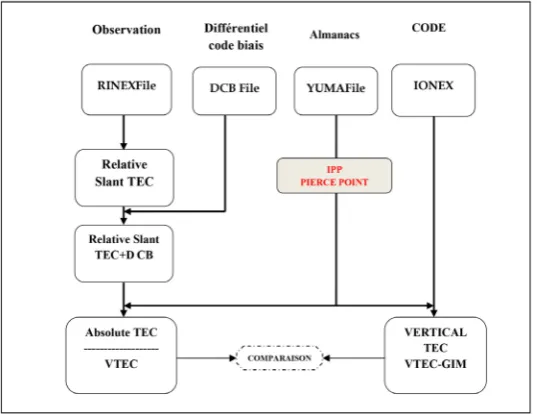
DOI: 10.4236/pos.2018.94006 84 Positioning (ECEF) coordinates, the satellite identification number and the time in GPS format. The algorithm for calculating the TEC is given in Figure 2. Calculation of the TEC from measurements of a station goes through the following steps:

1) RINEX format file: the RINEX (Receiver Independent Exchange) file con-tains the observations that make it possible to determine the local TEC or expe-rimental TEC denoted TEC GNSS. This data are downloads from the IGS web-site.

2) IONEX format file: the IONEX file (Ionosphere Exchange) contains the observations of the global TEC or theoretical TEC, denoted TEC GIM. This data are downloads from the website: ftp.unibe.ch [12].

3) Almanac file (yuma file): the almanac is the set of parameters allowing a priori the state, trajectory and clock bias of one or more satellites. Each almanac is linked to a GPS week number. It is valid for all GPS stations. It is retrieved from the website https://celestrak.com/GPS/almanac/Yuma/.

4) DCB file (Differential Code Biased): it gives all the satellite and receivers bias. It is valid for one month and for all GNSS stations, and is retrieved from the website: ftp.unibe.ch.

Above is an algorithmic diagram that illustrates methodology for computation of ionospheric delay:

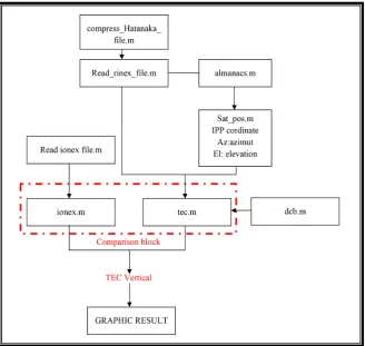
The process of extracting data from the RINEX file by using Matlab pro-gramming language. The program will analyze and extract the information needed to calculate the TEC. Figure 3 shows the main steps of extractions of raw data such as: observation Rinex file, ephemeris file, DCB file and Ionex file.

4. Results and Discussions

We calculated the monthly daily variation of the TEC of all data obtained during the days of the year. The months of a year are divided into four seasons: the

DOI: 10.4236/pos.2018.94006 85 Positioning

Figure 3. Subroutine Matlab for computing the vertical TEC.

equinox (March, April, September and October), winter (November, Decem-ber, January and February) and summer (May, June, July and August). An analysis of the results obtained from the two permanent stations of the IGS network was evaluated in relation to the geomagnetic activity through the magnetic index Ap. The magnetic index Ap (daily measurement of the distur-bance force in the Earth’s magnetic field) is extracted from the data of the web-site: http://isgi.unistra.fr/data_plot.php.

In Figure 4, we present values of the daily magnetic index Ap for the years 2001, 2009 and 2013, on the absciss axis are represented the day of the year and on the ordinates are represented the values of the index Ap. The AP index values greater than 25 correspond to magnetically disturbed days.

In order to interpret the geomagnetic effects in relation to the ionospheric ac-tivity, we began to study the behavior of the TEC according to the days classified in ascending order of geomagnetic activity (Table 1).

4.1. Data Description

DOI: 10.4236/pos.2018.94006 86 Positioning

Figure 4. Magnetic index AP of the year 2001, 2009 and 2013.

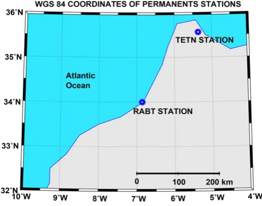
Figure 5. Locations of reference stations.

Table 1. Classification of geomagnetic activity according to the days of the year 2001-2009-2013.

DOY YEAR AP VALUES GEOMAGNETIC ACTIVITY

90-2001 2001 192 High

310-2001 2001 142 High

328-2001 2001 104 High

17-2013 2013 14 Average

121-2013 2013 26 Average

315-2013 2013 22 Average

270-2009 2009 2 Low

257-2009 2009 0 Low

DOI: 10.4236/pos.2018.94006 87 Positioning

4.2. Monthly Variation of the Ionosphere

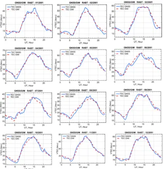
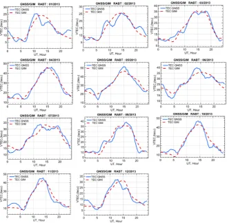
The diurnal variation of the TEC is attributed to daily rotation of the Earth. In order to determine the diurnal variation of the ionosphere, we calculated the TEC on the three specific years 2001-2009-2013. The results of a year with low solar activity year (2009) are presented in Figure 7, Figure 10, and Figure 11. Similarly for a year with a high solar activity (2001/2013) are represented in Figure 6, Figure 8, Figure 9 and Figure 11. The results are expressed in ordi-nate for VTEC (tecu) between 0 and 100 tecu and in abscisshour UT between 00 and 24. The blue curve represents the median VTEC values of the GNSS model and the red curve shows the median VTEC values of the GIM model. Later we will note VTEC-GIM for the GIM model and VTEC-GNSS for GNSS model.

Over the three years, the values of VTEC-GIM are in perfect agreement with those of VTEC-GNSS in all years studied. Both methods are on dual-frequency GPS observations. However, the TEC-GIM data was relatively smooth, whereas the TEC-GNSS values varied much faster in a short time. These results can be attributed to the different models used: the TEC-GNSS derived from a regional station (RABT/TETN), while the TEC-GIM was obtained from several global IGS stations.

DOI: 10.4236/pos.2018.94006 88 Positioning

Figure 7. The monthly medians of the VTEC for the RABT station, during the year 2009 located at least of the solar cycle 23. with the exception of February due to instrument failure.

During the two years 2001 and 2013, the solar power is strong and the TEC is gradually hanging over the time interval 08 and 12 UT and decrease between 16 UT and 24 UT, just before the sunset. The peak values are found in the range of 15 - 25 TECU for all the month and seasons in the tree year, between the period of 12 UT and 16 UT. In addition, the peak value of the TEC was much longer in this period than in others. The value of VTEC overnight (20 TU and 04 TU), remains very low compared to the mid-day. The Inflexion Point of the value of TEC was detected during the whole year (2001-2009-2013) between 4 UT and 8 UT. The values of the TEC between 12 UT and 16UT are very different during the tree years of measurement. The sunspot number is over 150 during the year of 2001 rather than 2013 the sunspot number are between 85 and 115, so lower than in 2001. The results obtained from the RABT a TETN station show that the monthly variations of VTECare affected by the solar radiations.

DOI: 10.4236/pos.2018.94006 89 Positioning

Figure 8. The monthly VTEC medians for the RABT station, during the year 2013 lo-cated at the maximum of the solar cycle 24. Cycle of low activity.

DOI: 10.4236/pos.2018.94006 90 Positioning

Figure 10. The monthly medians of Total Electron Content at TETN station during the year 2009.

2 tecu. What is not the case for the RABT station which has discrepancies going from 0 to 8 tecu. This is due to the RABT station which is closer to the south and therefore the VTEC values are stronger.

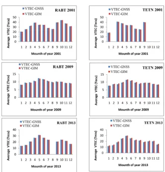
The maximum values of VTEC-GIM and VTEC-GNSS for two stations were observed at spring equinox (March and April) and winter equinox (October and

November). Figure 12 shows the monthly average VTEC values obtained by

different models at the RABT and TETN stations in 2001, 2009 and 2013. The values are calculated on average with all the TEC data collected during each month. In the three years, the monthly average TEC time series showed two peaks. In April-May and in September-October, The values of the TEC observed are greater at equinoxes, spring and winter, especially in the year of maximum solar 2001-2013. In 2009 solar minimum values of the TEC becomes more im-portant at the summer solstice (June). The minimum values of the TEC observed during the three years are those attributed to the month of January.

4.3. Seasonal Variation

DOI: 10.4236/pos.2018.94006 91 Positioning

Figure 11. The monthly medians of Total Electron Content at TETN station during the year 2013.

comparison purposes we have started to choose three seasons to examine the variation of the TEC and the intensity of connection between the two models, the equinox (March, April, September and October), winter (November, De-cember, January and February) and summer (May, June, July and August).

The correlation technique is used to mount if there is a strong connection between the models and if this connection is strong. The results of the correla-tion of the RABT stacorrela-tion are shown in Figure 13 and Figure 14 and for TETN station are shown in Figure 15 and Figure 16. The results showed that the cor-relation coefficient between the two models for the two stations during the two years 2001 and 2009 is very important (≈ 0.99), except for winter where it is 0.78 for the RABT station during the period 2009 Figure 14. This allows interpreting two things:

- As long as the coefficient is very positive, the VTEC-GNSS increases while the VTEC-GIM increases.

- the high intensity allows validating the reliability of the GIM model.

DOI: 10.4236/pos.2018.94006 92 Positioning

Figure 12. Monthly average values of VTEC for RABT and TETN stations in 2001, 2009 and 2013.

Figure 13. Correlation between the two models VTEC_GNSS and VTEC_GIM of the RABT station for the year 2001.

DOI: 10.4236/pos.2018.94006 93 Positioning

Figure 14. Correlation between the two models VTEC_GNSS and VTEC_GIM of the RABT station for the year 2009.

Figure 15. Correlation between the two models VTEC_GNSS and VTEC_GIM of the sta-tion TETN for the year 2001.

DOI: 10.4236/pos.2018.94006 94 Positioning

Figure 17. VTEC-GNSS, VTEC-GIM and AP index for the RABT and TETN station for the two years 2001 and 2009.

Table 2. WGS84 coordinates of reference stations.

STATION COUNTRY CITY LATITUDE (˚) LONGITUDE (˚) HEIGHT (M) RABT Maroc Rabat 33.9981

−

−

Table 3. Effect of geomagnetic activity on ionospheric error.

STATION DOY YEAR AP VTEC (tecu) IONO DELAY L1 (m)

RABT

90-2001 2001 192 66.48 10.79 310-2001 2001 142 93.43 15.17 328-2001 2001 104 No data No data 270-2009 2009 2 22.51 3.65 257-2009 2009 0 15.47 2.51 93-2009 2009 1 19.37 3.14

TETN

DOI: 10.4236/pos.2018.94006 95 Positioning

4.4. Geomagnetic Activity

From Figure 17, the calculation of VTEC is done for all days of the year. We opted to put a scale of comparison with the variation of the magnetic index to identify magnetic storms (Table 2). We took the average value of the VTEC for each day and plotted the result for the whole year.

A large variation in the maximum values of the parameters of the geomagnet-ic activity is observed between the two periods 2001 and 2009. According to our results presented in Figure 17, the values of the VTEC confirm the same varia-tion. This leads to the conclusion that the geomagnetic activity affects the TEC data largely during the period of high activity (2001) compared to the period of low activity (2009). Table 3 presents the result of calculation of the ionospheric error on the L1 band of the two GNSS stations during the two solar years 2001 and 2009.

5. Conclusions

In this study, we calculated the ionospheric TEC at the RABT and TETN station in year with high solar activity (2001) and year with low solar activity (2009). Then, we analyzed the diurnal variation, monthly variation, and solar depen-dence of the TEC. The main results are as follows:

- TEC value generally increased in the period of 07:00 to 10:00 UT inall sea-sons and was maximized in the period of 12:00 to 16:00 h UT.

- The maximum values of TEC were found during the equinox and winter for

both measurement years 2001 and 2009. In the first period of 2001 the max-imum values for RABT and TETN station ≈ 40 - 50 TECU, during the equi-nox and the minimum was found in the winter ≈ 12 - 17 TECU.

- The comparison between VTEC-GNSS and VTEC-GIM allowed us to

vali-date our methology for computing ionospheric VTEC. A strong correlation (≈0.99) between the VTEC-GNSS and VTEC-GIM has been found for all season except winter season (≈0.78) for RABT station in period 2009. There-fore, it maybe concluded that the TEC value will be maximum during equi-nox season which may be attributed to solar activity for each period.

- The effect of geomagnetic storm on the ionosphere provides a positioning

error ranging from 2.33 m to 15.17 m in period of low and high solar activity

Acknowledgements

I am grateful to Dr. Bouziani Mouradand Dr. Christine Amory-Mazaudiez for given me the study leave in Telecom Bretagne Institute to process ionosphere GPS data. I am immensely grateful to Dr. Rolland Fleury for his technical train-ing at matlab programmtrain-ing level. Authors thanks the International GNSS Ser-vice (IGS) and the Center for Orbit Determination in Europe, University of Berne (CODE) who made the RINEX files and IONEX files available.

Conflicts of Interest

DOI: 10.4236/pos.2018.94006 96 Positioning

References

[1] Warnant, R. (2006) l’effet de l’atmosphère terrestre sur les GNSS: Une perturbation ou un signal géophysique? Bulletin de la Société géographique de Liège, 47, 19-23. [2] International GNSS Service. ftp://cddis.gsfc.nasa.gov/gnss/products/

[3] Smith, C.A. (1987) Ionospheric TEC Estimation with a Single-Frequency GPS Re-ceiver. The Effect of the Ionosphere on Communication, Navigation and Surveil-lance Systems. Ionospheric Effects Symposium. Naval Research Laboratory. [4] Warnant, R. (1996) Etude du comportement du contenu électronique total et de

se-sirrégularités dans une région de latitude moyenne. Application aux calculs deposi-tions relatives par le GPS. Observatoire Royal de Belgique.

[5] Jin, R., Jin, S. and Feng, G. (2012) M_DCB: Matlab Code for Estimating GNSS Sa-tellite and Receiver Differential Code Biases. GPS Solutions, 16, 541-548.

https://doi.org/10.1007/s10291-012-0279-3

[6] Shukla, A.K., Neha, N., Saurabh, D., Nishkam, J., Sivaraman, M.R. and Bandyo-padhyay, K. (2008) Statistical Comparison of Various Interpolation Algorithms for Grid Based Single Shell Ionospheric Model over Indian Region. Journal of Global Positioning Systems, 7, 72-79. https://doi.org/10.5081/jgps.7.1.72

[7] Gao, Y. and Liu, Z.Z. (2002) Precise Ionosphere Modelling Using Regional GPS Network Data. Journal of Global Positioning Systems, 1, 18-24.

https://doi.org/10.5081/jgps.1.1.18

[8] Schaer, S. (1999) Mapping and Predicting the Earth’s Ionosphere Using the Global Positioning System. Thesis, University of Berne, Berne, 228 p.

[9] Seeber, G. (2003) Satellite Geodesy. 2nd Edition, Walter de Gruyter, Berlin, 589 p.

https://doi.org/10.1515/9783110200089

[10] Liu, J., Chen, R., Wang, Z. and Zhang, H. (2011) Spherical Cap Harmonic Model for Mapping and Predicting Regional TEC. GPS Solutions, 15, 109-119.

https://doi.org/10.1007/s10291-010-0174-8

[11] Davies, K. (1990) Ionospheric Radio. IEEE Electromagnetic Waves Series 31, Peter Peregrinus, London.