Bayesian and Non-Bayesian Estimation of the Inverse
Weibull Model Based on Generalized Order Statistics
Ahmed H. Abd Ellah
Department of Mathematics, Sohag University, Sohag, Egypt Email: [email protected], [email protected]
Received September 21, 2011; revised December 10, 2011; accepted December 20, 2011
ABSTRACT
The concept of generalized order statistics has been introduced as a unified approach to a variety of models of ordered random variables with different interpretations. In this paper, we develop methodology for constructing inference based on n selected generalized order statistics (GOS) from inverse Weibull distribution (IWD), Bayesian and non-Bayesian approaches have been used to obtain the estimators of the parameters and reliability function. We have examined Bayes estimates under various losses such as the balanced squared error (balanced SEL) and balanced LINEX loss functions are considered. We show that Bayes estimate under balanced SEL and balanced LINEX loss functions are more general, which include the symmetric and asymmetric losses as special cases. This was done under assumption of discrete-con- tinuous mixture prior for the unknown model parameters. The parametric bootstrap method has been used to construct confidence interval for the parameters and reliability function. Progressively type-II censored and k-record values as a special case of GOS are considered. Finally a practical example using real data set was used for illustration.
Keywords: Inverse Weibull Distribution; Generalized Order Statistics; Record Values; Progressive Type-II Censored; Balanced Type Loss Function; Bootstrap Estimation
1. Introduction
Udo Kamps [1,2] has introduced GOS as random vari-ables having certain joint density function, which includes as a special case the joint density functions of many models of ordered random variables such as ordinary order sta- tistics (OS) (David [3], Castillo [4] and Arnold, Balakrish- nan and Nagaraja [5]), sequential order statistics (SOS) (Cramer and Kamps [6,7]), record values, Kth record values, and Pfeifer’s records (Nevzorov [8] and Ahsanullah [9]), Progressive Type-II censoring order statistics (PCOS) (Soliman [10-13], Balakrishnan and Asgharzadeh [14], and Sarhan, Ammar and Abuammoh [15]). The structural similarities of these models are based on the similarity of their joint density function. Therefore, all of these mod- els are contained in the model of GOS.
For Bayesian estimates, the performance depends on the form of the prior distribution and the loss function assumed. The prior information can be expressed by the experi- menter, who has some belifs about the parameters of his parametric model. Traditionally, most authors use the sim- ple quadratic loss function and obtain the posterior mean as the Bayesian estimate. However, in practice, the real loss function is often not symmetric. For example, the cones- quences of overestimates, in loss of human life, are much more serious than the consequences of underestimates. In this case an asymmetric loss function is more appropriate.
Recently, many authors consider asymmetric loss func- tions in reliability, such as [Wahed [16], Alicja [17], Abd Ellah [18-20] and Sultan [21].
In this paper based on n selected GOS from the inverse Weibull model, we consider the problem of Bayesian and non-Bayesian estimation for parameters and reliability func- tion of the model. This was done under assumption of dis- crete-continous mixture prior for the unknown parameters. It well know that in Bayesian setting, for making opti- mum decision, importance should be given on the choice of loss function and not just the choice of prior distribu- tion. So, the results are presented under the balanced ver- sions of symmetric and asymmetric loss functions. Pro- gressively type-II censored and record values as a special case of GOS are considered. The rest of paper is organ- ized as follows. In Section 2, we first present some pre- liminaries.
2. Preliminaries
terpretation of the IWD in the context of the load-strength relationship for a component. Recently, Maswadah [24] has fitted the IWD to the flood data reported in Dumon- ceaux and Antle [25]. For more details on the IWD, see, for example Murthy et al. [26]. The two parameter IWD has probability density function (pdf) cumulative distri- bution function (cdf) and reliability function S(t) which are given respectively as
1
= exp , 0, ,
f x x x x > 0,
(1)
= exp
, 0, , > 0,F x x x (2)
and the reliability function at time t is
= 1 exp
, 0, , > 0,S t t t (3)
where and are scale and shape parameters re-spectively.
We recall the concept of GOS (cf. Kamps [1]).
Let n N n , 2and
1,1 2 1
= , , , n
n
m m m m
1, , , ,
then the random variables X n m k , X n n m
, ,, ,k
are called the generalized order statistics if their joint pdf is given by
, , 1 (1, , , ) ( , , , )
1 1
1 =1
, ,
= ,
X n m k Xn n m k n
n mi k
n i i i n
f x x
c F x f x F x f x
n
(4)
For 1
1
, where1
0 < n< 1
F x x F
1
1 =1 =1 =
= = , =
and = 1 .
n n n
n i i i i j i j i
c k k n j m
F x F x
2.2. Balanced Type Loss Functions
The class of balanced type loss function (BLF) we can write it in the form (see Ahmadi et al. [27]).
, , , = , 1 ,
q
L q q
(5) where estimating of parameter
, a prior target estimator of
,
0,1
,
, being as arbitrary loss function in estimating
by and q
suit-able positive weight function. In this paper we shall use balanced squared error loss (balanced SEL) and balanced LINEX loss function to illustrate Bayesian estimation of parameters of inverse Weibull.2.2.1. Balanced Squared Error Loss Function The balanced SLE is obtained with the choice of
2, =
, and q
= 1 in (5), and given by
2
2, , = 1
L
and the Bayes estimation of
under L ,
,
is given by
, x = x 1 E .
x
)
(7)
2.2.2. Balanced LINEX Loss Function
The balanced LINEX loss function with shape parameter
( 0
c c , is obtained with the choice of
, = c
1, e c
and in (5),
and given by
= 1q
, , = 1
1 1 ,
c
c
L e c
e c
(8)
and the Bayes estimation of
under L ,
,
is given by
,
1
= log c x (1 ) c .
x e E e
c
x
(9)
3. Maximum Likelihood Estimation (MLE)
Let X
1, , , , ,n m k
X n n m k
, , ,
are n GOS drawn from inverse Weibull distribution whose pdf is given by (1), based on this set of GOS the log-likelihood function is
=1 =1
1 =1
, = log ,
= ln ln 1 ln
ln 1 exp 1 ln 1 exp .
n n
i i i i
n
i i i n
x L x
n n x x
m x k
x
(10) If both of the parameters and are unknown, their MLEs, ˆML and ˆML can be obtained by solving the following likelihood equations
1 =1 =1
exp
1 exp
1 exp
= 0, 1 exp
n n i i i
i
i i i
n n
n
m x x
n x
x
k x x
x
(11)
1 1
=1 =1 =1
exp ln
ln ln
1 exp
1 exp ln
= 0. 1 exp
n n n i i i i
i i i
i i i i
n n n
n
m x x x
n
x x x
x
k x x x
x
ton-Raphson technique. By moving any point along in the direction determined by the information matrix and the first derivative of the log-likelihood function, we can iteratively improved the starting estimates to MLE, for details see Lawless [28]. For a given t, the corresponding MLE S tˆ
ML of the reliability function my be obtained by replacing
S t
and by ˆML and ˆML in (4).
3.1. Special Cases
In general, it is not easy to find a natural interpretation of generalized order statistics in terms of observed random samples. So, an interesting special cases such as the pro- gressive Type II censored order statistics and record val- ues have been used. These models are the most applica- ble general models of ordered random variables and is useful in reliability and life time studies. Several authors have addressed inferential issues based on progressive Type-II censored samples (for example, see Balakrishnan and Sandhu [14], Aggarwala and Balakrishnan [29] Ng et al. [30], Balakrishnan et al. [31] and Soliman [10-13]. One may refer to Balakrishnan [32,33] for a recent over- view of various developments relating to progressive cen- soring. Also, record values arise in a wide variety of practi- cal situations. Examples include industrial stress testing, meteorological analysis, hydrology, seismology, sporting and athletic events, and oil and mining surveys. Proper- ties of record values have been studied extensively in the literature. Interested readers may refer to the books by Nevzorov [8] and Arnold et al. [34,35].
In this section we will consider two special cases of GOS, namely, the progressively Type-II censored sample and lower record values.
3.1.1. Progressively Type-II Censored Data
A progressively Type-II censored sample is observed as follows: n units are placed on a life-testing experiment and only m≤n are completely observed until failure. The censoring occurs progressively in m stages. The m stages are failure times of m completely observed units. At the time of the first failure (the first stage), R1 of (n – 1) sur-
viving units are randomly withdrawn from the experi- ment, R2 of the (n – R1 – 2) surviving units are withdrawn
at the time of the second failure (the second stage) and so on. Finally, at the time of the mth failure (the mth stage), all the remaining (Rm – n – m – R1 – – Rm–1) surviv-
ing units are withdrawn. We will refer this to as progres-sively Type-II censoring scheme (R1, R2, , Rm) Then,
we shall denote the m completely observed failure times
by 1, ,
: : , = 1, 2, , . R Rm
i m n
X i m
The progressively Type-II censored sample
with censoring scheme and
1, ,
1: : , ,
R Rr n N
X
1
= , , Rn ,
1, ,
: : ,
R Rn n n N
X
n
R R
0,1 ,
i
R i
= ,
i i
m R
is a special case of the GOS with the parameters i= 1,2, , n1 and k=n=Rn1,
see Burkschat et al. [36].
From Equations (11) and (12) the required estimates
ˆ
ML
and ˆML in progressively Type-II censored are to be found by solving simultaneously the following two equations
1
=1 =1
exp
= 0, 1 exp
n n
i i i
i
i i i
R x x
n x
x
(13)
=1 =1 1
=1
ln ln
exp ln
= 0. 1 exp
n n
i i i
i i
n i i i i
i i
n
x x x
R x x x
x
(14)The ML estimate of reliability S t
is given byˆ
ˆ = 1 exp( ˆ ML),
ML ML
S t t (15) where ˆML and ˆML are be found from the numerical solution of the Equations (13) and (14).
3.1.2. Lower k-Record Values
Let
Xj, j1
be a sequence of independent andiden-tically (iid) continuous random variables with cumulative distribution function (cdf) F x
and probability density function (pdf) f x
. An observation Xj is defined to be an lower record if Xj< Xi for every and an analogous definition can be given for upper records ( with the inequality being reversed ). The record values is special case of GOS, in which if we put1
< .
i J
=
m1 m2= =mn = 1, and replacing F x
by F x
in (10), then the log-likehood of lower k-record values is given by
=1
, = ln ln ln 1 nln i n ,
i
x n k n n x kx
(16) the ML estimates of and can be obtained from (16) by solving the following two equations as then
=1
ˆ = , ˆ =
ln ln
.
ML n ML n
i n
i
n nkx
x n x
(17)The ML estimate of reliability S t
is given by
ˆˆ = 1 exp( ˆ ML),
ML ML
S t t (18) where ˆML and ˆML are given by (17).
4. Bayes Estimation
In this section, we estimate the two parameters and
considering both of balanced SEL and balanced LINEX loss function. Progressively type-II censored and k-re- cord values as a special case of GOS are considered.
4.1. Bayes Estimation Based on GOS
When both of the two parameters and are assumed to be unknown, Soland [37] considered a family of joint prior distributions that places continuous distributions on the scale parameter and discrete distributions on the shape parameter.
Suppose that the shape parameter is restricted to a finite number of values 1, 2, , with respective prior
probabilities 1, , ,2 such that 0j1,
=1 = 1 j j
and P
= j
= .j=
Further, suppose that conditional upon j, j= 1,2, , has a natural gamma
aj,
jb prior, with a density
1= = j aj exp , , , > 0.
j j j j
j
b
b a b
a j a (19)
by using the Bayes theorem, the conditional posterior density function of is given by
0
, ; =
= ,
, ; = d
j j j L x x L x j
(20)
1 1 1 =1 =1 = , =exp 1 exp ,
n a j j
m n
n i
j
i j i
i i
x A
x b x
j
11 exp ,
k j i x
(21)
where
1 1 1 1 1 1 1=0 =0 d=0
= n .
j n m m k j n a q q j
D n a A T
(22)On applying the discrete version of Bayes theorem, the marginal probability distribution of is given by
1 1 1 1 1 2=0 =0 d=0
= n ,
j n
aj n m
m k j j j j j
n a
q q
j j
b D n a
A
a T
= =
j j
p P x
(23)where
1 1 1 =1 1 1 1 2=1 =0 1=0 d=0
= , = , j n j j i i
aj n m
m n k j j j j j
n a j q qn
j j
x
b D n a
A a T
(24),
and .
1 1 1 11 1
1
= 1 q qn d n
n m m k D q q d
1=1 =1
= n j n j d j
j i i i n
i i
T
x
q x x bj (25)Bayes Estimation Based on Balanced S From (21) the Bayes estimates of
4.1.1. EL
and S t
, in
GOS under balanced SEL can be obtained, respectively as
1
1 1 1 1
ˆ = ˆ 1 m mn k j j ,
BS
p A D n a
1 1
1
=1 =0 n =0 d=0 j
ML n a
j q q
j T (26) ,
=1ˆ = ˆ 1
BS ML j
j
p j
(27)and
1 1 1 1 1 1=1 =0 =0 d=0
ˆ = ˆ
1 1 n
j n
BS ML
m
m k j
j n a
j
j q q
j
S t S t
D n a
p A
T t
,
(28) where ˆML and ˆML,
are to be found by solving (11) and (12), S tˆ( )ML A1, pj and T
j are given ress Estim on Ba
pec-tively, b 5), (22) 3) and (25).
4.1.2. Baye ation Based lanced LINEX Loss Function
y (1 , (2
From (21) the Bayes estimates of , and S t
in GOS under balanced LINEX loss function can be ob, respectively as
-tained
1 1 1 1 1 ˆ 1=1 =0 =0 d=0
1 ˆ =BL
c
log 1 n ,
j n
m
m k j j
c ML
n a j q q
j
p A D n a e T c
(29)
ˆ =1 1ˆ = log cML 1 c j
BL j j e p c , e
( and 30)
1 1 ˆ 1 =1 1 1=0 =0 =0 =1 1
1
ˆ = log 1 1
, ! BL n j n
cS t c
j BL
j s
m m k j
n a j
q q d s
j
S t e p A e
c
D n a c
s T st
(31)A1, pj and T
j ˆ( ) ,MLS t
and (12), are given
respec-tively, by , (23) and (2
4.2. Special
In this ion we will co o special cases of gos, the pr type-I d sample and lower record val
ro y T
(15), (22) Cases subsect ogressively ues. g l tions (2 5). nsider tw I censore (28) th 4.2.1. P ressive ype-II Censored Data
From Equa 6), (27) and e Bayes estimates of , and S t
in progressively type-II censored data under balanced SEL, are given respectively by
1 1 1 =1 =0 =01
= 1 ,
j n
BS ML n a
j q q
j T
n p A D3 1 (32)
1 R
R
j n aj
ˆ ˆ
ˆ ˆ 1 ,
=1
( ) =
BS ML j j
j
t t p
(33)
and
11 1 1 ... q j
0) and (3
3 =0 =0 ( ) n j n R R j n a j j q
D n a
p A
T t
And Fr tions (29), (3 1) timates of
=1
1 j 1
om Equa
ˆ( ) = ˆ
BS ML
S t S t
(34)
the Bayes
es-, and ogressively type-II er balan ss function, given respectively by
S t in pr ced LINEX lo censored data und
1 1 ˆ 1 c ML
3 1
=1 =0 1 ˆ = log . j BL R j j n a j q c
D n a
e T c
(35) =0 1 n n R qp A
j
ˆ =1 1ˆ = log c ML 1 c j ,
BL j
j
e p e
c
(36)and
1 1 ˆ 3 =1=0 =0 =1
1
1
ˆ = log 1
!
n
j n
cS tML c
j BL j s R R j n a j
q q s
S t e p A
c
a c
s t
1 1 j e D n T s ,
(37) re whe
1 1 1 1 4=0 =0 =1
1 = , ( ) n j n
aj n
R
R j n
j j j j j
j n a j
q q i
j
j
D n a
b
p A x
a T
= i ,
1 11
1
= 1q qn n
n R R D q q
11
=1 =1
= n j n j .
j i i i
i i
T
x
q x bjand
1 1 1 1 1 1 4=1 =0 =0
1 1 1 3 =0 =0 1 =
and = .
n
n
n
j n
aj n R
R
j j j j j
n a j
j q q
j j R R j n a q q j
b D n a
A
a T
D n a
A T
(38)ower k-Record Values
21), (22) and (27) in Lower k-record values the Bayes estimates of
4.2.2. L From (
, S t
and under balanced SEL, given respectively by
=1
ˆ = ˆ 1 j
BS ML j j
j n j
n a p
kx b
, (39)
=1
j n t bj
ˆ = ˆ
, j j j j BS ML n a n j
S t S t
kx b
1 pj 1
kx and (40) .
=1ˆ = ˆ 1
BS ML j
j
p j
Similarly From (21), (22) and (27) in Lower k-record values the Bayes estimates of
(41)
S t
and under balanced LINEX loss function respectively, are given
ˆ
=1
1
ˆ = log 1 .
j
j
n
cML n j
BL j
j n j
kx b
e p
c kx b c
j a
(42)
ˆ =1 1ˆ = log 1 1
! j j
cS tML c
j
s n j
S t e p e
s kx st b
=1 , j j BL j n a s n j c kx b
c
and
(43)
ˆ =1 1ˆ = log c jML 1 c j
BL j
j
e p
c
e ,
where
6
1 =1
=
and = .
j j
j
j
a n c
j j j j j
j n a
j j
n j
n
j i
i
n a
A b e
p
a kx b
x
(45)
5. Bootstrap Statistical Inference
The bootstrap is a resembling method for statis . It is commonly used to estimate confidence but it can also be used to estimate bias and vari-ance of an estimator or calibrate hypothesis tests. Boot-strapping is carried out by having an original data set
tical in-ference
tervals,
1, 2, , n
X X X
cumulative distributio
and sampling from an estima n function (cfd) of
te of the
1, 2, , n
X X X
The re-sam- i2, , Xin), i =
such that there pled
are H re-sampled data sets. data set will be denoted as Xi = (Xi1, X
1, 2, , H. Inferences for the quantity , where
is the vector of parameters, generally employ a test statistic, denoted as ˆ =T X X
1, 2, , Xn
. In order toestimate the sampling distribution of ˆ, two methods are employed, the nonparametric and parametric bootstrap methods. The parametric bootstrap method involves having a mathematical model whose parameters that completely probability density function (pdf) of 1,
determine the X
2, , n
X X , while the nonparametric one
there is not an explicitly given mathematical model to use, but it is assumed that the re-sampled data sets are independently and identically distribute he fol-
is used
d (iid). T lo
o
when
wing algorithm to describe the percentile bootstrap method as:
Algorithm A: Percentile bootstrap alg rithm
1) From an original data set X X1, 2, , Xn, draw H independent bootstrap samples X1,
2 X, ,
H
X with replacement, each of size n.
2) Compute ˆi and ˆ
i
, i = 1, 2,, H in progris-
seve type II censored from numerical solution of (13) and (14), and from numerical solution of (17) in lower record values.
3) Calculate the mean of all values in ˆ and ˆ.
4) Sort the values ˆ1, ,ˆH and ˆ ˆ
1, H
in
cend-in
boo strap con-as g order to obtain the bootstrap samples
ˆ[1], ,ˆ[ ]H
and
ˆ[1], , ˆ[ ]H
5) A two-sided 100 1
fidence interval for
% percentile t
and is defined, respectively, by
ˆH2, ,ˆ12H
and
ˆH2, , ˆ12H
(See Efron [38] and Efron et al. [39] for detailed dis-cu
In this section, xample have been included in an attempt to illustrate the use of lower record values and
pr censored in
6.1. Lower Record V E
Nelson [22], concerning the data on time to d between electrodes at a he 19 time to breakdown
Then the real data set from Inverse Wiebull
distribu-8, 0.124, 0.031, 0.136, 0.154, ssion).
6. Application Example
two e
ogressive type II estimating the parameter and reliability.
alues xample 1. (Real data)
We consider the real data set from Wiebull distribution as given by
breakdown of an insulating flui voltage of 34 KV (minutes). T are
0.96, 4.15, 0.19, 0.78, 8.01, 31.75, 7.35, 6.50, 8.27, 33.91, 32.52, 3.16, 4.85, 2.78, 4.67, 1.31, 12.06, 36.71, 72.89.
tion are
1.04, 0.24, 5.26, 1.2
0.121, 0.029, 0.0314, 0.32, 0.21, 0.36, 0.214, 0.76, 0.082, 0.027, 0.013.
Therefore, we observe the following lower record val-ues:
1.04, 0.24, 0.124, 0.031, 0.029, 0.027, 0.013.
We can obtain the values of
a bj, j
by using theexpected values of the reliability S t
;
1
exp =
j
aj aj
j j
b b
=
1 exp d
, > 0. j E S t
t
t
= 1 1
j j
j a
a t
j
b
(46)w suppose that the prior beliefs about the
distribu-tio
and
No
n enable one to specify two values
S t
1 ,t1
S t2 ,t2
. Then the values of j,bj are no used toa n by obtained numerically from (46). If there
ca
prior beliefs, a estimate the two etric approach can be
nonparam
values of S t
by using
=
= 0.625.0.25
i i
n i
S t X
n
See Martez and Waller [40].
By using the nonparametric approach of the reliability function ,
(47)
we set t1 = 0:.031 and t2 = 0.124 in (47), we get S(t1) = 0:5 and S(t2) = 0.36.
For =10 concerning the value of the MLE of the pa-rameter which be found by solving the Equation (17),
ˆ = 0.585
ML
Then the values of the hyper-parameters aj, bj at each example 1.
0 13; ; ; 0.0307; ; ; ;
0.1 ; 0.1 .1 21 4; 0 36; ;
1. 28 6. Thi dat c fro e I
W ll d tio t
value of j are obtained by solving the
tio thod.
following equa-ns using Newton-Raphson me
0.031
1 1 = 0.5,
j
j a
j
b
0.124
1 1 = 0.36.
j
j a
b
j
ws the values of the per-parameters and
Table 1 sho hy
posterior probabilities obtained for each j.
By using the algorithm A and the entr of Table 1, the boots p estimate, the ML estimate and the Bayes estimates of
ies tra
, , and S t
are presented in Table 2.By using a rd values in
Algo-rithm A the confidence intervals of the real d ta of lower reco
, , and S t
are presented in Table 3.
6.2. Progressive Type II Censored
Example 2. (Real data) We will take the same values in
ter nd the pos-te
Table 1. Prior information, hyper-parame s a rior probabilities.
j vj βj aj bj Pj vj 1 0.1 0.30 0.539. 2.182 0.116 0.0103* 2 0.1 0.35 0.440 1.775 139 0.26 3 0.1 0.40 0.375
0. 0*
1.508 0.145 0.0655* 4 0.1 0.45 0.327 1.320 0.137 0.1640*
122 0.4140*
7 0.1 0.60 0.242 0.984 0.083 2.6000*
0.208 0.854 0.050 10.600* 0 0. 0. 0. 40. * 5 0.1 0.50 0.293 1.180 0.
6 0.1 0.55 0.265 1.071 0.103 1.0400*
8 0.1 0.65 0.224 0.913 0.065 6.6000* 9 0.1 0.70
10 0.1 .75 195 803 038 100
*In ates u 4
Ta M ay bo p es s of
S( ith ω
ML Boot .)BS )BL
dic that the value m ltiply by 10 .
ble 2. t) w
The t = 0.5
L, B and
es and = 0.2.
otstra timate θ, β and
(.) (.) strap ( (.
0. 1
c = 5 c = c = 1.5
θ 550 737 420. 0. 0. 8 0.416 0.405 0.394
β 585 715 65 656 ) 562 45 45 451
0. 0. 0. 9 0. 0.652 0.649
S(t 0. 0. 3 0. 7 0. 0.445 0.439
confidence intervals of θ, Table 3. Two-sided 90% and 95%
β and S(t) by bootstrap estimate.
90% P. Interval Length 95% P. Interval Length
θ [0.0166, 0.1611] 1.1445 [0.0137, 1.2682] 1.2545
β [0. 1. 0. [0. 1.662 1.2495
S(t) [0.0515, 0.7914] 0.7399 [0.0391, 0.8252] 0.7861 4323, 5526] 1203 4133, 8]
.0 0.027 0.029 0.0314 0.082 0.121 24 36; 0 54; 0. ; 0.21 0.24; .32;0. 0.76 04; 1.
iebu
; 5.2 istribu
s n then
a have he
ome m th nverse MLEs of and , using a Newton-Raphson method are obtained as ˆ = 0.635814 and ˆ = 0.825806, so S tˆ
ML = 0.620 , at t = 0.6.e w pe l to e
va o ra
716
W ill use the ex cted va ue of S t
find th lues f the hyper-pa meters aj and bj for Known j , j=1, 2, ,10 .
t=0.0314 = 0.76
, and S
t= 0.214 =
0.40 , SThese two prior probabilities are substituted into (46), where aj and bj are solved numerically for each given
j
, j= 1, 2, ,10 using Newton-Raphson methods (in Table 4).
Table 5 shows the values of the hyp -param ers and er et posterior probabilities obtained for each j.
By using the algorithm the entries of Table 5, the b tstrap estimate, th estimate and the Bayes
A and
oo e ML
estimates of , , and S t
are prese in Table 6.t
nted
Table 4. Progressive ype II censored sample (m = 8, n = 9) from Nelson (1982).
i 1 2 3 4 5 6 7 8
xi,m,n 5.26 1.28 1.04 0.76 0.36 0.21 0.15 0.14
Ri 0 0 3 0 3 0 0 5
Table 5. Prior information and posterior probabilities.
j vj βj aj bj Pj vj 1 0.1 0.60 4.264 20.090 0.007 2.075*
2 0.1 0.65 2.364 11.459 0.029 2.635*
5 0.1 0. 067 5.681 5.392*
912 5. 846* 801 4. 691*
8 0.1 0.95 0. 4.226 0.143 11.035* *
10 0. 1. 0. 3. 0. 17. * 3 0.1 0.70 1. 8.296 0.063 3.345*
4 0.1 0.75 0.293 6.667 0.097 4.247* 661
80 1. 0.125
6 0. 7 0.
1 1
0.85 0.
0. 026
565 0.143 6.
8. 90 0. 0.148
715
9 0.1 1.00 0.648 3.970 0.130 14.009
1 05 594 773 113 786
*Ind tes tha alue ly b
Tab 6. Th L, B st m f θ
S(t) with t = and 0.2
p ica t the v multip y 103.
le e M ayes and boot rap esti ates o , β and 0.6 ω = .
(.)ML (.)Bootstra (.)BS (.)BL
c = 0.5 c = 1 c = 1.5
θ 0.635 0.7213 0.547 0.542 0.538 0.534
β 0.825 0.
S 0. 0.
8322 0.869 0.867 0.864 0.862
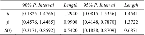
Table 7. Tw ded and 95% c nc rv β and (t) by bootstr stimate
95% P. Interval Length
o-si 90% onfide e inte als of θ,
S ap e .
90% P. Interval Length
θ [0.1825, 1.4766] 1.2940 [0.0815, 1.5356] 1.4541
β [0.4576, 1.4485] 0.9908 [0.4148, 0.7870] 1.3722
S(t) [0.3171, 0.8592] 0.5420 [0.1838, 0.8709] 0.6871
B using e real ata of rogr ty sam le in Algorithm A the confid
y th d p essive
ence in pe II ce
tervals nsored
of
p ,
, and ar nt Ta
E
C
neralized Order Statistics,
[2] U. ra of
l-ize ,” ic ,
269 0 8
S t e prese ed in ble 7.
REF REN ES
[1] U. Kamps, “A concept of Ge Teubner Stuttgart, 1995,
”
. Kamps and E. C mer, “On Distributions Genera d Order Statistics Statist s, Vol. 35, No. 3 2001, pp
-280. doi:10.108 /023318 0108802736
[3 . r S s w
York, 1981. [4]
ew York, 1992.
[6] E. Cramer an al Order Statistics
and k-Out-of-n ally Adjusted Fa
] H A. David, “Orde tatistic ,” 2nd Edition, Wiley, Ne
E. Castillo, “Extreme Value Theory in Engineering,” Academic Press, Boston, 1988.
[5] B. C. Arnold, N. Balakrishnan and H. N. Nagaraja, “A First Course in Order Statistics,” Wiley, N
d U. Kamps, “Sequenti
Systems with Sequenti
il-ure Rates,” Annals of Institute of Statistical Mathematics, Vol. 48, No. 3, 1996, pp. 535-549.
doi:10.1007/BF00050853
[7] E. Cramer and U. Kamps, “Marginal Distributions of Sequential and Generalized Order Statistics,” Metrika, Vol. 58, No. 2, 2003, pp. 293-310.
doi:10.1007/s001840300268
[8] V. B. Nevzorov, “Records,” Theory of Probability and Its Applications, Vol. 32, No. 2, 1987, pp. 201-228.
doi:10.1137/1132032
[9] M. Ahsanullah, “Record Statistics,” Nova Science Pub-lisher, Inc., Commack, New York, 1995.
[10] A. A. Soliman and G. R. Elkahlout, “Bayes Estimation of the Logistic Distribution Based on Progressively Cen-sored Samples,” Journal of Applied Statistical Science, Vol. 14, 2005, pp. 281-293.
[11] A. A. Soliman, “Estimation of Parameters of Life from Progressively Censored Data Using Burr-XII Model,” IEEE Trans. Reliab, Vol. 54, No. 1, 2005, pp. 34-42. doi:10.1109/TR.2004.842528
[12] A. A. Soliman, “Estimations for Pareto Model Using General Progressive Censored Data and Asymmetric Loss,” Communications in Statistics Theory & M Vol. 37, No. 9, 2008, pp. 1353-1370. ethods, doi:10.1080/03610920701825957
[13] A. A., Soliman, A. H. Abd Ellah, N. A. Abou-Elheggag and A. A. Modhesh, “Bayesian Inference and Prediction of Burr Type XII Distribution for Progressive First Fail-ure Censored Sampling,” Intelligent Information
Man-agement, Vol. 3, 2011, pp. 175-185.
, No. 1, 2005, pp. 73-87.
e Using Burr Model
tion under
Asym-ential Distribution Using Record
Observa-yesian and Non-
ed on Record
Val-. Nelson, “Applied Life Data Analysis,” John Wiley
pplicata, Vol. 2, No. 1, 1990, pp.
lation, Vol. 73, No. 12, 2003, pp. [14] N. Balakrishnan and A. Asgharzadeh, “Inference for the Scaled Half-Logistic Distribution Based on Progressively Type-II Censored Samples,” Communications in Statis-tics Theory & Methods, Vol. 34
[15] A. M. Sarhan and A. Abuammoh, “Statistical Inference Using Progressively Type-II Censored Data with Random Scheme,” Int. Math. Forum, Vol. 3, No. 33-36, 2008, pp. 1713-1725.
[16] A. S. Wahed, “Bayesian Inferenc
Under Asymmetric Loss Function: An Application to Carcinoma Survival Data,” Journal of Statistical Re-search, Vol. 40, No. 1, 2006, pp. 45-57.
[17] J. R. Alicja, “A Sequential Estimation Procedure for the Parameter of an Exponential Distribu
metric Loss Function,” Statistics & Probability Letters, Vol. 78, No. 17, 2008, pp. 3091-3095.
[18] A. H. Abd Ellah, “Bayesian Prediction of Weibull Dis-tributions Based on Fixed and Random Sample Size,” Serdica Mathematical Journal, Vol. 35, 2009, pp. 129- 146.
[19] A. H. Abd Ellah, “Parametric Prediction Limit for Gener-alized Expon
tions,” Applied Mathematics & Information Science, No. 2, 2008, pp. 135-149.
[20] A. H. Abd Ellah, “Comparison of Estimates Using Re-cord Statistics from Lomax Model: Ba
Bayesian Approaches,” Journal of Statistical Research of Iran Statistical Research and Training Center, Vol. 3, No. 2, 2006, pp. 139-158.
[21] K. S. Sultan, “Bayesian Estimates Bas
ues from the Inverse Weibull Lifetime,” Model Quality Technology & Quantitative Management, Vol. 5, No. 4, 2008, pp. 363-374.
[22] W. B
& Sons, New York, 1982.
[23] R. Calabria and G. Pulcini, “On the Maximum Likelihood and Least Squares Estimation in the Inverse Weibull Dis-tribution,” Statistica A
53-66.
[24] M. Maswadah, “Conditional Confidence Interval Estima-tion for the Inverse Weibull DistribuEstima-tion Based on Cen-sored Generalized Order Statistics,” Journal of Statistical Computation and Simu
887-898. doi:10.1080/0094965031000099140
[25] R. Dumonceaux and C. E. Antle, “Discrimination be-tween the Lognormal and Weibull Distribution,” Tech-nometrics, Vol. 15, 1973, pp. 923-926.
doi:10.2307/1267401
[26] D. N. P. Murthy, M. Xie and R. Jiang, “Weibull Model,”
s of Distributions under Balanced Type Loss John Wiley & Sons, New York, 2004.
[27] J. Ahmadi, M. J. Jozani, E. Marchand and A. Parsian, “Bayes Estimation Based on k-Record Data from a Gen-eral Clas
Functions,” Journal of Statistical Planning and Inference, Vol. 139, No. 3, 2009, pp. 1180-1189.
Life-03.
Balakrishnan ods and Applications of Probability time Data,” John Wiley & Sons, New York, 20
[29] R. Aggarwala and N. Balakrishnan, “Maximum Likeli-hood Estimation of Laplace Parameters Based on Pro-gressive Type-II Censored Samples,” In: N.
Ed., Advances in Meth ,
and Statistics, Gordon & Breach Publishers, New York, 1999.
[30] H. K. T. Ng, P. S. Chan and N. Balakrishnan, “Optimal Progressive Censoring Plans for the Weibull Distribu-tion,” Technometics, Vol. 46, No. 4, 2004, pp. 470-481. doi:10.1198/004017004000000482
[31] N. Balakrishnan, N. Kannan, C. T. Lin and H. K. T. Ng, “Point and Interval Estimation for Gaussian Distribution Based on Progressively Type-II Censored Samples,” IEEE Transactions on Reliability, Vol. 52, No. 1, 2003, pp. 90-95. doi:10.1109/TR.2002.805786
[32] N. Balakrishnan, “Progressive Censoring Methodology: An Appraisal,” Test, Vol. 16, No. 2, 2007, pp. 211-259. doi:10.1007/s11749-007-0061-y
[33] N. Balakrishnan and R. A. Sandhu, “A Simple Simula-tional Algorithm for Generating Progressive Type-II Cen-sored Samples,” American Statistician, Vol. 49, No. 2, 1995, pp. 229-230. doi:10.2307/2684646
[34] B. C. Arnold, N. Balakrishnan and H. N. Nagaraja,
Linear
Estima-eralized Pareto
“Re-cord,” Wiley, New York, 1998.
[35] B. C. Arnold and S. J. Press, “Bayesian Estimation and Prediction for Pareto Data,” Journal of the Acoustical So-ciety of America (JASA), Vol. 84, 1998, pp. 1079-1084. [36] M. Burkschat, E. Cramer and U. Kamps, “
tion of Location and Scale Parameters Based on General-ized Order Statistics from Gen
tions,” In: M. Ahsanullah, Ed., Recent Developments in Ordered Random Variables, Nova Science Publisher, New York, 2007, pp. 253-261.
[37] R. M. Soland, “Bayesian Analysis of the Weibull Process with Unknown Scale and Shape Parameters,” IEEE Tran- sactions on Reliability, Vol. R18, No. 4, 1969, pp. 181- 184. doi:10.1109/TR.1969.5216348
[38] B. Efron, “Censored Data and Bootstrap,” Journal of the American Statistical Association, Vol. 76, No. 374, 1981, pp. 312-319. doi:10.2307/2287832
[39] B. Efron and R. J. Tibshirani, “Bootstrap Method for Standard Errors, Confidence Intervals and Other Meas-ures of Statistical Accuracy,” Statistical Science, Vol. 1, No. 1, 1986, pp. 54-75. doi:10.1214/ss/1177013815 [40] H. F. Martz and R. A. Waller, “Bayesian Reliability