Hardware design of a cooperative adaptive cruise control system using a functional programming language

(1)

August 18, 2014

MASTER’S THESIS

Hardware design of a

cooperative adaptive

cruise control system

using a functional

programming language

T.A.W. (Erwin) Bronkhorst, BSc.

Faculty of Electrical Engineering, Mathematics and Computer Science (EEMCS)

Chair: Computer Architecture for Embedded Systems (CAES)

Graduation committee: Dr. ir. J. Kuper

(2)

(3)

Acronyms

CλaSH CAES Language for Synchronous Hardware

ACC Adaptive Cruise Control

CACC Cooperative Adaptive Cruise Control

CAES Computer Architecture for Embedded Systems

FPGA Field-programmable Gate Array

GHC Glasgow Haskell Compiler

HDL Hardware Description Language

MPC model predictive control

PID Proportional Integral Derivative

RTL Register-transfer Level

VHDL VHSIC Hardware Description Language

(6)

(7)

Abstract

In this master’s thesis a relatively new hardware design approach is used to model a CACC (Co-operative Adaptive Cruise Control) system. In the traditional hardware design flow, a problem description is made in an imperative language like C and after verification it is rewritten to a hardware description language like VHDL or Verilog. After this step, new verification and sim-ulations are performed and finally, the actual hardware is implemented. In this approach a lot of transformations are involved, which are very time consuming and error-prone.

The new design approach used in this investigation uses a mathematical description given in the functional programming language Haskell to verify the correctness of the model. After that the Haskell code is slightly modified to be compiled into VHDL code using the so called CλaSH (CAES Language for Synchronous Hardware) compiler. This is a compiler developed in the CAES (Computer Architecture for Embedded Systems) group, which translates code that is written in a subset of Haskell into fully synthesisable VHDL code. This enables the possibility to implement the system on an FPGA (Field-programmable Gate Array).

(8)

(9)

Chapter 1 Introduction

The evolution in technology causes an increasing demand of energy-efficient and at the same time powerful hardware for the calculations in several embedded systems. This demand can not always be satisfied by doing most calculations on general purpose hardware like an ordinary desktop computer, for which the algorithms are written in software. In order to satisfy these demands, it is possible to design hardware which is developed especially for the embedded tasks and which is dedicated to do these calculations. With the increasing complexity of these embedded systems, it becomes harder to go through the design and verification process for the hardware design of these systems. The complexity makes the steps that must be taken in this process very time-consuming and errors can easily arise. In both hardware and software design, a programming language is used to describe the system that is to be designed. While there are a lot of similarities in design approach, there are also some big differences. In hardware design there are some constraints that should be taken into account and which are not common to purely software design, like set up and hold times, input and output buffers and many timing constraints. Therefore there are programming languages developed which focus purely on the design of hardware by giving the designer more control over these things.

A major cause for the challenges in hardware design, is that the traditional hardware de-scription languages, like VHDL and Verilog, lack a high level of abstraction. Unfortunately a high level of abstraction could make the design a lot easier, because the designer can focus on the behavioural part of the system and a lot less on the actual implementation in hardware. A promising method to deal with these problems and to introduce more abstraction to the design flow, is to use a functional programming language. One of the main properties of a functional programming language is that is a high-level language with a high level of abstraction, which is beneficial for productivity. Using this kind of language, the implementation in the programming language stays close to the actual problem description and system behaviour. Another major ad-vantage of using a functional programming language for hardware design, is that there is a direct relation between the functional description of an algorithm and the hardware that implements this algorithm. This relation is not that strong when using an imperative language to describe the system. This is mainly caused by syntactic constructs that are hard to analyse mathematically, like for-loops and assignment-statements.

(10)

INTRODUCTION

language like C. The model is than simulated and verified in for example MATLAB or Simulink. After these steps, the actual hardware design is performed in a hardware description language like VHDL and verified again. With a hardware design approach using a functional program-ming language, the transition from the functional language to a hardware description language can be more intuitive.

In the CAES group at the University of Twente, a tool is developed that generates fully synthesisable VHDL code from a specification written in the functional programming language Haskell using a subset of this language. This tool is called the CλaSH-compiler. This tool gives the opportunity to describe a system at a high abstraction level by describing its mathematical properties using functional expressions. By describing a problem description in a functional programming language, the simulations on the system can be done without any transformations to a programming language with other semantics. The direct transformation from the description in Haskell to a hardware description in VHDL also eliminates the need for a manual conversion step which can introduce errors in the system.

Since functional programming languages are well suited to describe systems purely with their mathematical equations, this method looks promising to describe a cyber-physical system. These are systems with computational units that control physical behaviour, for example by using sensor information and controlling actuators. The support for higher-order functions in a functional language enables some extra possibilities. One could think of different step sizes for integration methods, depending on the requirements for that specific calculation. In the traditional way of simulating these systems, one global step size is defined. If at one place a high precision in terms of timing is required, than the whole simulation will get that precision. This will lead to long simulation times, or it will require very powerful hardware to do the simulations.

In this research, a simulator of a cyber-physical system will be implemented in Haskell and the result will be compiled using the CλaSH-compiler to investigate if this design method is suitable to describe a cyber-physical system. This leads to the following research question:

• To what extend is a hardware design method using a functional programming language suitable for the simulation and implementation of cyber-physical systems?

While looking for the answer to this question, we will investigate how the system can be extended, for example to increase the accuracy and make it more realistic by adding extra pa-rameters. The easier it is to make these modifications, the better the hardware description can be maintained in production environments. This will save time and costs during further de-velopment and improvement of a system. Furthermore, there will be investigated if the use of higher-order functions can indeed optimize the simulations so less processing power is required to get the same or a better precision.

(11)

INTRODUCTION

acceleration or break strength of the predecessor. By using this information as a feed forward in the controller, the following distance can be made shorter without losing string stability [1]. This increases the vehicle capacity of the road. In this investigation, a simulator of a CACC system will be developed to verify the behaviour of the controller.

The developed the simulator consists of two major parts: the vehicle model and the con-troller. The car model consists of a state variable, which includes the position, speed, accel-eration and jerk of the vehicle. The controller uses this state and the state of its predecessor as inputs and calculates a desired acceleration to minimize the distance, speed and acceleration error. When the vehicle is controlled to accelerate at this desired value, the state of the current vehicle is changed, resulting in changing inputs of the controller. When a correct controller is used, an equilibrium is reached in which the errors are (almost) zero.

The structure of this report is as follows. First, a brief introduction on CACC will be given, followed by a full mathematical analysis of a CACC system. When this mathematical back-ground is given, an explanation of the process of designing hardware using a functional pro-gramming language is discussed. After that, a description of the implementation is Haskell will be given, ending with the results of the simulation in Haskell.

(12)

(13)

Chapter 2 Background

In this chapter, the required background information on CACC is given, followed by the math-ematical analysis of the CACC system that will be used. Next, the process of hardware design using a functional language is discussed. After that, an implementation of the CACC system in Haskell is presented.

2.1 Cooperative Adaptive Cruise Control

A big issue on busy roads, are traffic jams. There are campaigns that ask people not to travel during peak hours and to travel together in one car, but they don’t have the desired effect. This raises the demand for a technical solution. If the amount of cars can not be reduced, the vehicle throughput of the road must be increased to solve the traffic jams. This can be done by reducing the inter-vehicle distance, but this will immediately lead to unsafe situations caused by the slow response time of human beings. To overcome this slow response time, a technical solution can be introduced, which controls the throttle and brake of the car. An implementation of such a system which is used more and more these days, is ACC. The goal of such a system is to keep a constant distance to its predecessor, or to keep a constant speed if the constant distance could only be achieved if the maximum speed must be exceeded. Using this technique, it is possible to create a vehicle string with all cars driving safely in the platoon while being comfortable for the passenger in the car [2].

ACC systems are developed to increase the comfort of the driver. There is less interference of the driver with the system required, due to the ‘adaptive’ component in the cruise control. But for a cruise control system that increases the throughput of the road, a shorter following distance must be applied while maintaining safety. This can be achieved if the ACC system is expanded to a CACC [3]. The difference between these systems, is that CACC uses inter-vehicle communication to transmit the current desired acceleration of a vehicle directly to its follower using wireless communication. When this information is used as an extra feed forward signal in the controller of the ACC system, the inter-vehicle distance can be reduced even more [4].

(14)

BACKGROUND 2.1 Cooperative Adaptive Cruise Control

spacing policy and it is similar to human behaviour. The time distance between two vehicles is calledheadwayand it causes a longer physical inter-vehicle distance at higher speeds. This longer distance can be used as a “buffer” between the vehicles to prevent collisions in case of sudden and fast speed changes of the preceding vehicle. Most spacing policies use a combination of physical distance and time headway. The desired physical distance is than calledstandstill distanceand this is added to the time headway to calculate the desired distance while driving at a certain speed.

Keeping the right distance to its predecessor is the main objective of the CACC controller and it is often referred to as individual vehicle stability. Besides this one, there is a second control objective: maintaining string stability. For a vehicle string to be string stable, there must be a guarantee that fluctuations in the speed of a car are attenuated upstream. This means that following cars should have fewer fluctuations than the preceding car in terms of the signal norm of for example speed [5] [6]. The string stability of a vehicle platoon is very important to prevent the generation of phantom traffic jams. These jams occur when a car breaks too strong, which causes its follower to break even harder to prevent a collision. This behaviour propagates backwards through the traffic, where finally cars will stand still. If a vehicle platoon is string stable, the inter-vehicle time headway is chosen in such a way, that a following car may always break less hard than its predecessor without colliding.

When designing a CACC system, there are two approaches. The first one is designing a centralized system which tells each individual vehicle how to behave. This kind of system gath-ers the relevant data of all vehicles in a certain area and calculates the best possible behaviour. Such a system requires a lot of information exchange between vehicles and the central system. Therefore, another approach is used which makes use of a decentralized system, where each vehicle gathers the relevant data by itself and calculates its own desired output.

2.1.1 Related work

There is a lot of active research in the subject of CACC systems. When looking into the existing literature in the subject of ACC and CACC, most studies focus on controller design. Some inves-tigations focus on the used control method or algorithm to get better results in terms of stability, others focus on better comfort for the user of the system. A lot of investigations analyse the cruise control systems when several non-idealities are added, like packet loss in the communi-cation. Others try to improve the model by using multi-vehicle look-ahead. String stability and individual vehicle stability is very important in all these investigations.

(15)

2.1 Cooperative Adaptive Cruise Control BACKGROUND

Communication delay and packet loss

A very important part of a CACC system, is dealing with delays. A CACC system uses sensors which introduce delays to the system [9]. Furthermore, wireless communication will introduce two negative factors to the system. First, there is a communication delay between the transmis-sion of the signal and the reception of this signal. In 2001, Liu et al. investigated the effects of communication delays on the string stability of a vehicle platoon [10]. The delays in wireless communication are caused by the calculations of the signal processing units and packet losses during the transmission. These packet losses result in absence of the data or delays due to re-transmission, depending on the used techniques. The delays in the system are random, which makes it hard to deal with them in a convenient way. Especially in platoons where a vehicle receives information from the platoon leader and its predecessor, these delays have big influence on the string stability of the platoon. Liu et al. propose a solution using synchronization of the in-formation exchange. Using this method, each vehicle in the string uses the received inin-formation simultaneously. This makes the delays effectively constant rather than random. Unfortunately, this will require all vehicles to use the same delay which will be larger than the actual delay.

In 2013, Ploeg et al. investigated the packet losses introduced by the communication [11]. Normally, a CACC system degrades to an ACC system in case of packet loss. This will require the time headway to increase but the result will stay string stable. Ploeg et al. present an alterna-tive fall-back method in which the desired acceleration of the preceding vehicle is estimated and used as an input parameter for the CACC controller. Experimental results showed that using this method, the time headway could be kept smaller in case of packet loss, compared to the method where degradation to an ACC system is used.

Two-vehicle look-ahead

Most systems use one-vehicle look-ahead, where only information of the direct predecessor is used. However, there exists research on two-vehicle look-ahead or a system which uses infor-mation of the platoon leader to further increase the performance of the system.

(16)

BACKGROUND 2.1 Cooperative Adaptive Cruise Control

given.

In the same year, Hallouzi et al. also published a paper which discussed two-vehicle look-ahead in cruise control systems [13]. In this investigation, another control law was used which defines two separate control goals. The fist one tries to minimize the position error to its direct predecessor, the other goal was to minimize the position error to the predecessor of its predeces-sor. Both separate controllers give a desired accelerationaref,2andaref,1respectively as output and based on these two desired acceleration the actual desired accelerationaref for the vehicle is calculated. If one or both predecessors are breaking, the desired acceleration is defined equal to the hardest breaking vehicle. If none of the vehicles is breaking, the desired acceleration is defined as the mean ofaref,2 andaref,1, or the desired accelerationaref,2 calculated from its direct predecessor if that desired acceleration is larger. Some extra intelligence is implemented to enable a smooth transition from one situation to another. The control method is verified with two experiments with three vehicles. In both experiments, the leading vehicle drove three differ-ent speeds for a while. The difference between the two experimdiffer-ents was that in one experimdiffer-ent one of the speeds was 0, so the leading vehicle did a stop and go manoeuvre. The results of the experiments were compared to the behaviour of real human drivers and it turned out that the automatic control with two-vehicle look-ahead performed better in terms of reaction time and passenger comfort. Also in this investigation, no comparison with one-vehicle look-ahead control algorithms is made.

A quantitative comparison between two-vehicle and one-vehicle look-ahead is performed in the master’s thesis of Kreuzen in 2012 [14]. In this investigation, two different control tech-niques are used: PID (Proportional Integral Derivative) and MPC (model predictive control)1. In this investigation, a two-vehicle look-ahead method using MPC was compared to MPC with one-vehicle look-ahead and with PID. During the investigation it turned out that PID had a smoother and more comfortable response due to less acceleration and jerk, but during one of the experiments it caused a collision. Therefore, the investigation mainly discusses on MPC and the influence of the performance and behaviour of the system using two-vehicle look-ahead with that control method. In this investigation, there are two different look-ahead techniques mentioned. The first one takes information of the two direct predecessors into account, the other one uses information of the direct predecessor and the platoon leader. The conclusions of the investigation teach that the system performs better when the information of two direct predeces-sors is used, because the behaviour of the second predecessor can be seen as information from the near future. For PID, two-vehicle look-ahead also had a positive influence. The best results were achieved by using information from the platoon leader and the direct predecessor. What must be noted here, is that the collision with the PID controller was of huge influence by de-ciding which option is better. The overall response using PID was smoother and therefore more comfortable than the response when using MPC, at the cost of response time. Due to the fact that PID responded slower, a collision occurred. In real life, safety is found more important than comfort, so MPC was labelled as the best option.

In a very recent publication of Ploeg et al., there is a two-vehicle look-ahead control strategy 1

(17)

2.2 Mathematical model of a CACC system BACKGROUND

mentioned [15]. The main focus in this paper is directed to a design method in which string stability requirements can be explicitly included. The one- and two-vehicle look-ahead analysis is used to illustrate the potential of this design method. Simulations of both variants show that two-vehicle look-ahead only performs better than one-vehicle look-ahead in terms of minimal time headway if the communication delay is large. For short communication delays (which barely increases with the physical distance), the minimal time headway was even larger than without two-vehicle look-ahead. The exact cause of this behaviour is not clear, but it seems to be related to the small error in information at low communication delays. It is also plausible that not the optimal control parameters were used. The used parameters were a result of optimisation and is not proven that this was the best solution for this problem. The authors recommend to actively switch between one- and two-vehicle look-ahead communication in a system, depending on the latency in the wireless communication at that specific moment.

Special traffic situations

In practice, there are many more situations than only driving in a single string of vehicles. While most researchers focus on pure platooning of vehicles in one string, there is some research going on that looks into special but very common situations in actual traffic. These special cases are not taken into account in this master’s thesis, but it is important to keep these situations in mind. Therefore, some literature on this subject is discussed here.

In 1999, Darbha and Rajagopal investigated the effect of vehicles that want to enter a vehicle platoon, for example at an access road. Before a vehicle could enter a platoon the platoon should increase the inter-vehicle distance at some place, so the extra vehicle can insert the platoon there. Several simulations were performed where vehicles enter and leave the vehicle platoon and the researchers were unable to find a constant time headway spacing policy which leads to a string stable platoon. Some recommendations have been proposed for future work, which makes use of a different spacing policy.

Another example of such a situation is the crossing of two vehicle platoons, which is in-vestigated by Diab et al. in 2012 [17]. An intersection management system is developed in this investigation, which takes over the control of the leading vehicle in a platoon at a crossing. While there was already some research done on intersections of automated platoons, this investigation claims to be the first that treats each platoon as a whole, opposing to older systems which try to control each vehicle individually. By using the control mechanisms of the platoons itself, this system makes sure that the intersection is passed as efficient as possible, without causing acci-dents or deadlocks. The researchers managed to get a working model and verified its behaviour by using a scale model of actual vehicles.

2.2 Mathematical model of a CACC system

(18)

BACKGROUND 2.2 Mathematical model of a CACC system

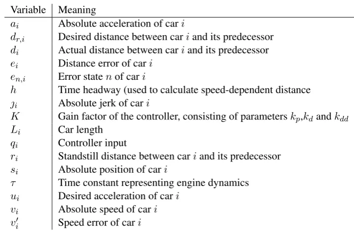
Given a string ofmvehicles, the desired distancedr,iof a vehicle to its predecessor can be defined as

dr,i(t) =ri+hvi(t), 2≤i≤m (2.1) In this equation,riis the standstill distance to the preceding car andviis the velocity of vehicle i. Theh is the time headway, which defines a speed dependent following distance. All used variables used in this section, are also presented in Table 2.1.

For the simulation later in this research, the distancedibetween two cars has to be expressed in terms of their absolute positions. The absolute positionsi of a car is defined as the position of the back of the car. With these definitions, the spacing errorei(t)can be defined as

ei(t) =di(t)−dr,i(t)

= (si−1(t)−si(t)−Li)−(ri+hvi(t)) (2.2) In this equation,Liis the length of vehiclei.

According to this equation, the car is too far from its predecessor if the spacing error is positive. A schematic overview of the used distances and positions are shown in Figure 2.1.

di di+1

di+2 i+1 i i-1 di-1

si+1

si

si-1

Li

Li+1 Li-1

[image:18.595.105.533.361.444.2]

ri hvi ei

Figure 2.1:Schematic overview of a string of vehicles [19]

For the vehicle model, three quantities are important: the distancedi to the predecessor, the speedvi of the vehicle and the accelerationai of the vehicle. These quantities will be the basis for the controller design. In the state space representation of a dynamic system, the time derivative of the state of the system at timetis expressed in terms of the state at timetand a control input [20]. To get the state space model of this CACC system, the time derivatives of the previous mentioned quantities should be calculated, resulting in

 

˙

di

˙

vi

˙

ai

 =

 

vi−1−vi ai −1_τai+_τ1ui



, 2≤i≤m (2.3)

In this equation, τ is a time constant representing engine dynamics andui is the desired acceleration. This is an input for the system: the car that is controlled.

(19)

the definition:

 

e1,i e2,i e3,i

 =   ei ˙ ei ¨ ei  =  

si−1−si−Li−ri−hvi vi−1−vi−hai ai−1−ai−ha˙i



, 2≤i≤m (2.4)

The second and third error state are respectively the first and second order time derivative of the spacing error function. Therefore, they can be expressed in the speed, acceleration and jerk of vehiclei. The second and third element from the error state vector represent the speed difference and acceleration difference between the car and its predecessor.

To construct a state space matrix, the time derivative of each error stateen,i must be ex-pressed in the state variables. From (2.4) it can be extracted that the time derivativee˙1,iequals e2,iand the time derivativee2˙ ,iequalse3,i. The time derivativee3˙ ,ican be calculated by substi-tutinga˙i from (2.3) into the expression of the error state. The derivatives of the different error states are

˙

e1,i= ˙ei =e2,i (2.5)

,

˙

e2,i= ¨ei =e3,i (2.6)

and

˙

e3,i= ...

ei

= (...s_i−1− ...

s_i)−(h...v_i) = ( ˙ai−1−a˙i)−h¨ai

= ((−1 τai−1+

1

τui−1)−(−

1

τai+

1

τui))−(h(−

1

τa˙i+

1

τu˙i))

=−1

τ(ai−1−ai+ha˙i)−

1

τ(hu˙i+ui) +

1

τui−1

=−1 τe3,i−

1

τqi+

1

τui−1 (2.7)

In (2.7), a new variableqiis defined. This is the input of the actual controller and is defined as

qi,hu˙i+ui (2.8)

This inputqi should stabilize the error dynamics of all states and compensate for the fluctu-ations inui−1: the input of the preceding vehicle. While each error state has to reach the value 0 eventually, the control law forqiis

qi=K

 

e1,i e2,i e3,i



(20)

BACKGROUND 2.2 Mathematical model of a CACC system

, with feedback gain factorK = (kp kd kdd). The values forK have a great influence on the dynamic behaviour of the system. This is primary used to get the desired behaviour (follow the preceding vehicle with a constant time distance) and string stability, but also to get comfortable behaviour. By choosing low values of K the amount of jerk is reduced, resulting in a more comfortable ride.

When substituting the inputqi in (2.7), the expression for the third error state can be con-structed as

˙

e3,i=−

1

τe3,i−

1

τ(kpe1,i+kde2,i+kdde3,i+ui−1) +

1

τui−1

=−1

τkpe1,i−

1

τkde2,i−

1

τ(1 +kdd)e3,i−

1

τui−1+

1

τui−1

=−kp τ e1,i−

kd τ e2,i−

1 +kdd

τ e3,i (2.10)

Now, the time derivative of each error state is expressed by means of the error states and a new state variableui, which is the desired acceleration of vehiclei. When (2.9) and (2.8) are combined, an expression of the time derivative ofuican be made in terms of all state variables. This leads to the expression

˙

ui =−

1

hui+

1

h(kpe1,i+kde2,i+kdde3,i) +

1

hui−1 (2.11)

With all state variables known and the expressions for their time derivatives, the state space system can be constructed:

   

˙

e1,i

˙

e2,i

˙ e3,i ˙ ui     =     

0 1 0 0

0 0 1 0

−kp

τ −

kd

τ −

1+kdd

τ 0 kp h kd h kdd h − 1 h         

e1,i e2,i e3,i ui     +     0 0 0 1 h    

ui−1 (2.12)

This system expresses how each state variable changes over time, based on the current state and the inputui−1, which is the desired acceleration of the preceding vehicle. The expression

from (2.12) will now be implemented to create the simulator.

In some situations, it is preferred to express the states in terms that have a pure physical meaning. In the state space model of (2.12), the state is expressed in errors of the position, speed and acceleration and there is still a termui, which is the desired acceleration and not the actual acceleration. Therefore, the model is changed to contain only the absolute speed, acceleration and jerk. The absolute position is always changing, except when the cars are not moving. Therefore, this state variable will be the distance error. This expression is already shown in (2.2). The time derivative of this expression is shown in (2.3).

(21)

substituteu˙i, giving a new expression with variables qi andui. The first one is substituted by (2.9) (with the expressions for the errors given in (2.4)) and the second variable again by (2.3):

˙

i = ¨ai =−

1

τi+

1

τu˙i

=−1 τi+

1

hτ(qi−ui)

=−1 τi+

1

hτ(kpe1,i+kde2,i+kdde3,i−(τa˙i+ai))

=−1 τi−

1

hτ((τa˙i+ai))+

1

hτ(kpei+kd(vi−1−vi−hai) +kdd(ai−1−ai−ha˙i) + (τa˙i−1+ai−1))

=−1 τi−

τ hτi+

1

hτai+ kp

hτei+ kd hτvi−1−

kd hτvi−

kdh hτ ai+

kdd hτai−1−

kdd hτ ai+

τ

hτi−1+

1

hτai−1− kddh

hτ i

= kp

hτei− kd hτvi−

1 +kdh+kdd hτ ai−

h+τ +kddh hτ i+

kd hτvi−1+

1 +kdd hτ ai−1+

1

hi−1 (2.13) With all time derivatives of the state variables known, the state space equation can be repre-sented via a matrix:

    ˙ ei ˙ vi ˙ ai ˙ i     =    

0 −1 −h 0

0 0 1 0

0 0 0 1

kp

hτ −

kd

hτ −

1+kdh+kdd

hτ −

h+τ+kddh hτ         ei vi ai i     +    

0 1 0 0

0 0 0 0

0 kd hτ

1+kdd hτ 1 h        

ei−1 vi−1 ai−1 i−1

   

(2.14)

A final remark that should be made here, is that to be able to do a good analysis on the string stability of the platoon, all state variables should become 0 in the desired state. Therefore, the absolute speedvi is converted to a speed errorv0i. This speed error is defined as the speed difference with the steady state speedveq, resulting in the expression

(22)

BACKGROUND 2.3 Hardware design using a functional language

This change of a variable does not change anything in the values of the state space matrices. This can be shown if the equations of (2.14) are written out, while substitutingviwithv_i0+veq. The negative occurrence ofveq in thevi part of the equation always cancels out the positive occurrence ofveq in thevi−1 part. This holds as long asveq is equal for all vehiclesi, which is the case by definition. When looking into the time derivative ofv_i0, one will notice that this derivative is the same as the time derivative ofvi as long asveq is constant. This is important, because the time derivatives are used in the calculations for the second state variable. So under the assumption thatveq is constant and the same for all vehicles, the values in the state space matrices of (2.14) will not change. Ifveqis chosen to be0, the speed error equals the absolute speed of the vehicle, which makes analysis more convenient.

[image:22.595.131.492.281.520.2]

All used variables and quantities used in this section, are summarized in Table 2.1.

Table 2.1:Overview of used variables

Variable Meaning

ai Absolute acceleration of cari

dr,i Desired distance between cariand its predecessor di Actual distance between cariand its predecessor ei Distance error of cari

en,i Error statenof cari

h Time headway (used to calculate speed-dependent distance i Absolute jerk of cari

K Gain factor of the controller, consisting of parameterskp,kdandkdd Li Car length

qi Controller input

ri Standstill distance between cariand its predecessor si Absolute position of cari

τ Time constant representing engine dynamics ui Desired acceleration of cari

vi Absolute speed of cari v_i0 Speed error of cari

Now we have a state space equation with state variables that have a direct physical meaning which can be used in simulations to get a good feeling of the dynamic behaviour of the system.

2.3 Hardware design using a functional language

(23)

2.3 Hardware design using a functional language BACKGROUND

semantics is used, so effectively the system description is written twice or even more if domain-specific calculations are required in for example Simulink. This takes a lot of time, because after each translation the code to another language, there are several verifications and simulations that need to be performed to check for new errors that were introduced in the transformation steps.

A more efficient way of designing hardware is enabled with the CλaSH compiler. This compiler is able to generate fully synthesisable VHDL code from a specification written in a subset of Haskell code. A large advantage of this design method, is that the verification and simulation of the designed system can be performed in Haskell. After the transformation to VHDL, the implementation corresponds with the Haskell description and therefore there is no intensive simulation and verification step required. This makes the design process less error prone and the development time much shorter.

Another big advantage from a developer’s point of view, is that the hardware description in a functional language like Haskell stays very close to the mathematical description of the algorithm. This makes the hardware description intuitive and relatively easy to debug.

2.3.1 Related work

For already a long time, the idea of designing hardware using a functional programming lan-guage exists. In the early eighties, there already were some researchers with the idea of de-scribing hardware in a functional programming language to improve design time and making the process of designing and verification more easy [21]. Some studies already indicated that a functional programming language could be very useful in designing and verifying hardware, for example due to its lazy evaluation and the equational description of systems [22]. Since that time, several projects have started to make hardware design using a functional programming language possible. This means that there are some alternatives to CλaSH, which is used in this investigation. In some of these projects, a completely new language is created. More often, an embedded language is developed which makes use of an existing functional programming language, mostly Haskell. Examples of functional languages that are used to design hardware, are ForSyDe [23], reFLect [24], Hawk [25], Lava [26] and CλaSH [27]. Since developing a HDL based on a functional programming language is quite a hard and time consuming task and because of the fact that this approach is not yet wide spread, some projects fail to grow out to a solid and full working language. Some other projects evolve into new ones, where the successor deprecates the predecessor. This means that at this moment, not a single “best language” can be nominated. Furthermore, there is a slight difference in application of each language. Some languages are only meant to design and verify hardware, but not to actually implement it. Oth-ers provide a way to actually build the hardware, for example CλaSH by compiling the code to synthesisable VHDL code.

(24)

BACKGROUND 2.4 Functional language representation

VHDL, there is a fundamental difference between the two. This difference is that CλaSH uses the language Haskell itself to describe the hardware, rather than the embedded language pro-vided by Lava. This enables the use of certain language-specific constructs like case-statements and pattern-matching, which is not possible when using Lava [27].

2.4 Functional language representation

For the developed simulation environment, Haskell is used. In this section, a description is given about how the simulation environment is developed. First, the core simulation is given, which calculates the new error states based on the previous error states. Subsequently the simulator is expanded with some functions, which calculates the actual position, speed and acceleration based on the error states.

2.4.1 Core model

The first step is to define how a car in the vehicle string is represented. The car has to store its own state ((ei, v0i, ai, i)T) and for programming purposes the index of the car within the vehicle string. For easy analysis of the behaviour of the vehicle, the absolute position and speed of the car are stored. Not all cars have the same length and therefore the length of the car is also stored as a property in the vehicle representation. In Haskell, a new data typeCarTypeis constructed by using the record syntax. This type definition is shown in Listing 2.1.

data CarType = Null |

Car { carid :: Int,

position :: Float,

speed :: Float,

carLength :: Float,

state :: [Float] } deriving (Show,Eq)

Listing 2.1:The definition of a CarType

Besides the constructCar, there is aNull without any property. Later on, you will find some functions that require the predecessor of a vehicle as an input parameter. The leading vehicle does not have any predecessor and to deal with that, this Null value is used as the input parameter for the predecessor.

In (2.14), the state change of a vehicle at a certain moment is calculated based on the current state of that vehicle and its predecessor. Define the new stateS0 at time t+ ∆tas a function of the stateS at timetand the state changeS˙ on the interval[t, t+ ∆t). This state change is a function of the state at timetand the state of the preceding car at time t. In a discrete time system, the time derivative of the state is multiplied by the sample time∆tand added by the current state to get the new state. So if the current state, the sample time and the state change are known, the new state can be calculated using the forward Euler method:

(25)

2.4 Functional language representation BACKGROUND

Using this method, the new state of a vehicle can be calculated in Haskell with the function

drivefrom Listing 2.2.

drive :: CarType -> [Float] -> (CarType,[Float])

drive car predState = (car’,state’) where

car’ = car {position = pos’, speed = speed’, state = state’}

Car { state = stateCar,

position = posCar,

speed = speedCar} = car

state’ = zipWith (+) stateDiff stateCar where

stateDiff = map (*dt) dstate

dstate = zipWith (+) (mxv a0 stateCar) (mxv a1 predState)

(_:v’:_) = state’

pos’ = (speed’+speedCar)*0.5*dt + posCar

speed’ = veq + v’

Listing 2.2:Calculation of the new state based on the current state

Thisdrivefunction gets aCarand the state of its predecessor as an input, and it returns a

tuple of two elements: the newCarand the new state of thisCar. This new state is also present in the returnedCaritself, but returning it a separate value in the tuple makes it easier in CλaSH to use it as an output.

In thedrivefunction, the variablesa0anda1are the matrices from (2.14). This imple-mentation makes use of a functionmxv, which performs a matrix vector multiplication.

The state of eachCarconsists of four state variables. Two of these variables are the absolute acceleration and jerk, but there are no state variables for the absolute position and absolute speed. In some situations, it is useful to have this information too. As can be seen in Listing 2.1, aCar

has support for the storage of the absolute position and absolute speed. These values must be calculated separate from the error state. The absolute speed is calculated by adding the steady state speed veq to the speed error and the absolute position is calculated with time integration of the absolute speed. Due to the discrete time domain, the integral is calculated using the midpoint rule. This is chosen different from the forward Euler method used for the calculation of the new state, because the midpoint rule is more precise than the forward Euler method and all information required for the midpoint rule is known here. All the mentioned calculations are performed in the last three lines of thedrivefunction.

To calculate the state change, a matrix-vector multiplication is performed. A matrix vector multiplication is in fact a vector multiplication mapped over all rows in a matrix. This means that each for each row in the matrix the dot product with the given vector is calculated and the result forms the new row, which than consists of one element. In Haskell this is done with the

mapfunction, which applies the function.*. ysto all elements ofxss. The function.*. ysis a dot product with vectorys2. The matrixxssis implemented as a list of rows, so one

2

(26)

BACKGROUND 2.4 Functional language representation

element ofxssis one row of the matrix, which is again a list.

To execute a dot product, eachnth element of the first vector is multiplied by thenth element of the second vector and the sum of all these products is the result of the dot product. The multiplication is translated to azipWith (*)function in Haskell and the sum of each element translates to a foldl (+) function. The resulting implementation of the dot product and matrix vector multiplication is shown in Listing 2.3 [29].

mxv :: [[Float]] -> [Float] -> [Float]

mxv xss ys = map (.*. ys) xss

(.*.) :: [Float] -> [Float] -> Float

xs .*. ys = foldl (+) 0 (zipWith (*) xs ys)

Listing 2.3:Matrix vector multiplication in Haskell

When a string of vehicles is defined as a list ofCars, the string can be simulated for one period∆twith thedrivePlatoonfunction, which is shown in Listing 2.4.

drivePlatoon :: [CarType] -> (Float,Float) -> ([CarType],[[Float]])

drivePlatoon cars (spdDes,accDes) = (cars’,map state cars’) where

cars’ = firstCar’ : rest’

firstCar’ = fixFirst.fst $ drive (head cars) [0,

spdDes - veq, accDes, 0]

rest’ = map drive’ $ zip (tail cars) cars

drive’ (myCar,predState) = fst $ drive myCar (state predState)

fixFirst car = car {state=(0 : tail (state car))}

Listing 2.4:Simulation of a vehicle string for one∆t

The previously mentioneddrivefunction requires the current car and the state of its pre-decessor as an input. Therefore the firstCar from list of Cars is removed with the function

tailand thanzipped with the complete list. The result is a list of tuples which are used as an input for a helper functiondrive’, which calls the functiondrivewith the current vehicle and the state of its predecessor and returns the new state of the vehicle (rest’). If thezip

function gets two list of different length (tail cars is one smaller thancars), there are tuples created as long as possible. If one of the lists is out of elements, the rest of the elements of the other list are discarded. In this case, the result of thezipfunction is a list of tuples with length equal totail cars.

(27)

2.4 Functional language representation BACKGROUND

drivePlatoonfunction. The other state variables are set to 0. By using this state variable as

an input for the calculations of the first vehicle, the new state of this vehicle can be calculated. Due to the fact that this is the leading vehicle it can also not have a position error, so the first state variable representing the position error is set to 0 after calculation. With these steps, the new instance of the firstCaris placed in front of the new instance of all otherCars (rest’).

To make an endless simulation of a vehicle string, thisdrivePlatoonfunction is called repeatedly to get a simulation over time. Each time sample is a list of cars and the whole time is a list of these lists of cars. Thesimulatefunction that does this, is shown in Listing 2.5. The parameternindicates the starting value of the time. In most simulations, this will be set to 0. In the developed simulator, there is a functiondesiredSpeed nand a functiondesiredAcc n which return respectively the desired speed and acceleration at time n. By changing these functions, the desired speed and acceleration at any time can be defined. In most situations, the functiondesiredAccis implemented as a time derivative of thedesiredSpeedfunction, but it is also possible to implement it as the exact function of the time derivative using the analytical time derivative of the input function.

simulate :: Float -> [CarType] -> [[CarType]]

simulate n cars = cars’ : simulate (n+dt) cars’ where

cars’ = fst (drivePlatoon cars (desiredSpeed n,desiredAcc n))

Listing 2.5:Simulation of a vehicle string over time

2.4.2 Simulation

To run an actual simulation of a vehicle string, the following steps are taken. At t = 0, the vehicle string is created. To do this, the position, speed and acceleration of each vehicle has to be defined. With these values, the error state of each vehicle can be calculated using the information of the preceding vehicle. The state variables of each vehicle in the string are calculated by using (2.4), except for the jerk. This state variable will always be 0 for each vehicle at the start of a simulation. Due to the fact that the first vehicle has no predecessor, the state variables must be calculated in a different way. The position of this first car is the actual position of the whole vehicle string and therefore, the position error of this vehicle will start at 0 and stay 0 forever. The speed error is calculated with respect to the output of the functiondesiredSpeedat time 0. In equilibrium, each car will drive at a constant speed and therefore the acceleration will be 0. The acceleration error is thus equal to the actual acceleration of the car. The same holds for the jerk error.

A vehicle can be added to the tail of a vehicle string using the addCar function. The parameters of this function are the length of the new vehicle, the vehicle string and the position, speed and acceleration of the new vehicle at timet= 0. With this data, a new vehicle string is created and returned. The Haskell code that implements this function is shown in Listing 2.6.

(28)

BACKGROUND 2.5 Simulation results

addCar :: (Float,Float,Float) -> Float -> [CarType] -> [CarType]

addCar (pos,spd,acc) myLength cars = cars ++ [car] where

Car {carid = carId,

position = posLast} = last cars

state’ = [e’,v’,a’,j’]

e’ = posLast - pos - myLength - ri - h*spd

v’ = spd-veq

a’ = acc

j’ = 0

car = Car {carid = carId + 1,

position = pos,

speed = spd,

carLength = myLength,

state = state’

}

Listing 2.6:Adding a car to a vehicle string

2.5 Simulation results

To verify the correct behaviour of the controller, the system is simulated in the interactive Haskell interpreter of GHC (Glasgow Haskell Compiler). The simulation parameters are chosen in such a way, that the correctness and behaviour of the model is verified. Four simulations are performed, with increasing complexity. This allows us to analyse the behaviour of the system step by step and remarkable behaviour is spotted faster.

[image:28.595.110.521.103.273.2]

For all simulations, some realistic values for the different constants in the model are used. Most of these values are taken from [18]. The values for the k-constants are chosen to get a realistic speed of response and optimal passenger comfort. The value of h is based on the minimal required time distance for string stability. The values are shown in Table 2.2.

Table 2.2:Overview of used constants in the simulation

Constant Value Unit

ri 2 m

Li 4 m

h 0.7 s

τ 0.1 s

kp 0.2

kd 0.7

kdd 0

∆t 0.01 s

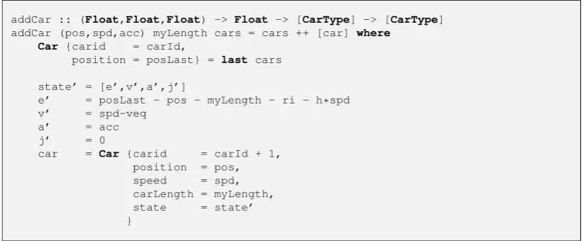
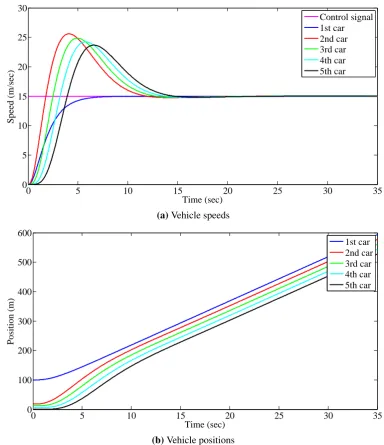
With these parameters, a simulation is performed with a vehicle string of five cars. All cars start with a speedvi = 0at timet= 0. The starting position of the front car is100, the starting position of the second car is18and each next car is placed 6 meter behind its predecessor (12,

(29)

2.5 Simulation results BACKGROUND

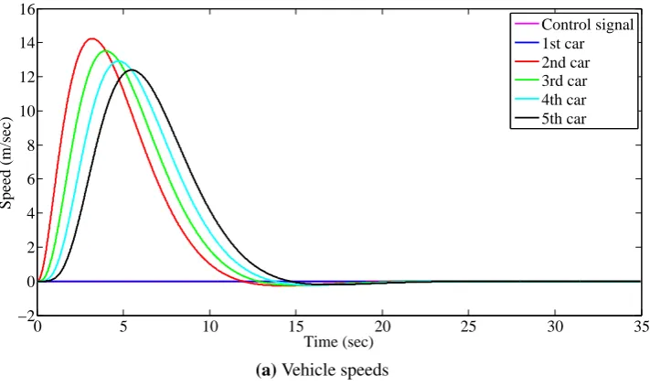
speedveqis kept at 0. This will cause the first vehicle to stand still. The second vehicle is too far behind its predecessor, so it will start driving towards the first vehicle. This will cause all other vehicles to drive as well, until all vehicles stand still at a standstill distance equal to 2 (ri). The simulation results are shown in Figure 2.2.

0 5 10 15 20 25 30 35

−2 0 2 4 6 8 10 12 14 16

Time (sec)

Speed (m/sec)

Control signal 1st car 2nd car 3rd car 4th car 5th car

(a)Vehicle speeds

0 5 10 15 20 25 30 35

0 10 20 30 40 50 60 70 80 90 100

Time (sec)

Postition (m)

1st car 2nd car 3rd car 4th car 5th car

[image:29.595.89.471.174.618.2]

(b)Vehicle positions

Figure 2.2:Behaviour of the controlled vehicle string with desired speed 0 as input.

(30)

lower than its predecessor, except for the first vehicle of course, because it is standing still. In Figure 2.2b there is a bit overshoot visible in which the vehicles come too close to their predecessor. This corresponds to in a negative speed: the cars are driving backwards. This seems bad in a real environment, but it is expected that when the cars have a speed larger than 0 at steady state, they will not end up driving in reverse.

To verify the behaviour of the vehicle string in the case where the desired speed is larger than 0, a new simulation is run. In this case, the starting positions remain unchanged and also the starting speeds are kept at 0. However, the functiondesiredSpeedis set to a constant value of 15m/s. The simulation results are shown in Figure 2.3.

As you can see, each vehicle will increase its speed, based on the distance to the preceding car and the speed error compared to the steady state speedveq. In Figure 2.3b the effect of a time headway as spacing policy is also visible. This can be seen when looking at the distance between the vehicles at the steady state, which is larger than in the steady state of Figure 2.2b, where the speed was 0. It is also visible when looking att = 0 andt > 20 in Figure 2.3b, because att= 0the cars are placed at standstill distance while their speed is0.

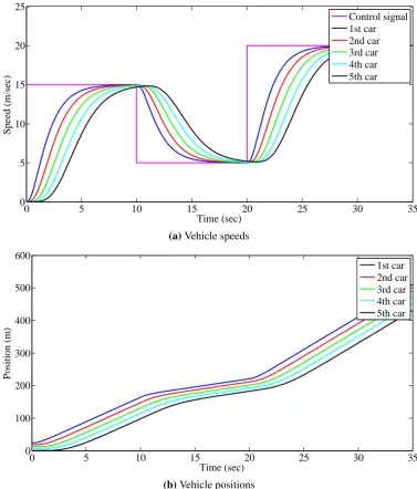
In the previous simulations, the control signal was fixed to one speed. However, the system must be able to change between different desired speeds. To verify the behaviour of the system in these cases, all vehicles are placed at standstill distance of each other, with a starting speed of 0. The last vehicle will have position 0 and each next vehicle will have an absolute position that is 6 more. This results in a starting position of 24 for the leading vehicle. Some different speed steps are used as input, to verify the correctness of the speed dependent following distance. The results of this simulation are shown in Figure 2.4.

With these values, the system still seems to be string stable and the inter-vehicle distance is indeed speed dependent.

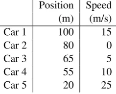
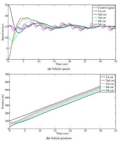
[image:30.595.255.374.511.607.2]

With the last simulation that is performed with the written Haskell code, several different cases at once are tested. Therefore, the start conditions of the vehicles in the string are changed. The used start values are shown in Table 2.3.

Table 2.3:Start conditions of each vehicle

Position Speed (m) (m/s)

Car 1 100 15

Car 2 80 0

Car 3 65 5

Car 4 55 10

Car 5 20 25

With these starting values, some vehicles need to reduce the distance to their predecessor, some others must increase it.

Furthermore, the control signal dictating the desired speed is changed to the randomly cho-sen periodic function

(31)

0 5 10 15 20 25 30 35

0 5 10 15 20 25 30

Time (sec)

Speed (m/sec)

(a)Vehicle speeds

0 5 10 15 20 25 30 35

0 100 200 300 400 500 600

Time (sec)

Position (m)

[image:31.595.86.471.105.551.2]

Figure 2.3:Behaviour of the controlled vehicle string with desired constant speed as input.

, which consists of a high and a low frequency component. The average of this signal is15, so the value forveqstays15. The simulation results of this experiment are shown in Figure 2.5.

It is visible in the image that each vehicle starts to correct for its incorrect starting values. After about 2.000 time samples (20 seconds) the system is stable and each vehicle follows its predecessor at the correct speed.

(32)

0 5 10 15 20 25 30 35

0 5 10 15 20 25

Time (sec)

Speed (m/sec)

(a)Vehicle speeds

0 5 10 15 20 25 30 35

0 100 200 300 400 500 600

Time (sec)

Position (m)

[image:32.595.126.504.107.550.2]

Figure 2.4:Response of the controlled vehicle string with different speed steps.

a lower speed, so Car 3 has to slow down to prevent collision. Also Car 4 slows down a lot and the main reason for that is that its distance to Car 3 is very short. The car slows down to let this distance increase and after a while, the speed is increased to get to the desired speed.

(33)

0 5 10 15 20 25 30 35

0 5 10 15 20 25

Time (sec)

Speed (m/sec)

(a)Vehicle speeds

0 5 10 15 20 25 30 35

0 100 200 300 400 500 600 700

Time (sec)

Position (m)

[image:33.595.88.472.156.614.2]

(34)

(35)

Chapter 3 Implementation method

The developed functional language representation in Section 2.4 is used as reference for the CλaSH code. However, before the CλaSH compiler is able to generate VHDL from the Haskell code, it should be modified. In the following section, these modifications are discussed. When the CλaSH compatible Haskell code is explained, the compilation to VHDL is discussed, fol-lowed by the simulations performed on the VHDL code in QuestaSim. The last part of this chapter focuses on the synthesis of the VHDL code.

3.1 Modifications to the Haskell code

While the CλaSH compiler can compile “normal” Haskell code, some changes must be made before it can be translated to a real hardware description[30]. The reason for this, is that hardware puts some limitations on the design and in some cases the efficiency in terms of FPGA area usage can be increased. In the following subsections, two important changes to the Haskell code are discussed.

3.1.1 Floating-point to fixed-point

In the developed program in Section 2.4, the most used data type is a single precision floating-point number. It is possible to implement floating-floating-point calculations in hardware, but it requires a lot more hardware compared to fixed-point calculations. The design choice for floating-point numbers in the program from Section 2.4 is for the precision of the values. The program uses meters and seconds as units of measurement and the control system requires more precision than that. It is also possible to achieve the required precision by using fixed-point numbers.

(36)

IMPLEMENTATION METHOD 3.1 Modifications to the Haskell code

The second thing to take care of, is that no integer overflow should occur. If too few bits are used for the integer part of the fixed-point number, a large value of the integer part will overflow and become a negative value. This should never happen, because the system will get undesired behaviour which can have a great impact on the safety of the driver. Therefore, the integer part should be large enough to represent the highest possible integer value within the simulator. The same holds for large negative numbers, which might underflow from negative to positive.

The last important design choice is the number of bits used for the fractional part of a fixed-point number. The more bits are used in this part, the more precision can be achieved. When the precision is too low, errors are introduced in the calculations. These errors might influence the calculations later on, because they use the result of the previous calculations. To deal with this effect, it is important to keep the precision at the required level.

For the implementation of the simulator, a single data type for all occurrences of a floating-point number is chosen. This will have implications for the efficiency of the program, because sometimes more precision is required and sometimes a higher value for the maximum integer value. To be able to deal with both situations, the length of the fixed-point number will be higher. However, using one data type makes it easier to do calculations between domains. For example, if the speed is represented in fixed-point number with different dimensions than time, a conversion should be made before the speed can be converted to a distance with integration. To eliminate these conversions, a fixed-point number is used which is large enough for all situations. In the developed simulator, the position of the car will have the highest value for the integer part of the fixed-point number. A problem is that the absolute position has virtually no limit if the car keeps driving in one direction. While the speed and acceleration have a physical limitation on their value (at some point, a car can not drive or accelerate faster), there is no such limitation for the absolute position. Fortunately, the value for the absolute position is only used to show the behaviour of the car and is not used in the calculations. In these calculations, only the position error is used and this value is for example bounded by the range of the lidar and the range of the wireless transmitter.

The boundaries on the speed, acceleration and jerk of the car are determined by the con-troller. The control parametersKof the controller are chosen in such a way, that the acceleration and jerk should not exceed the comfort boundaries. In 1977 an investigation is performed on the comfort values for the acceleration and speed of a vehicle [31]. This investigation pointed out that a jerk that exceeds 3 m/s3and an acceleration higher than 2 m/s2are considered uncomfort-able, although sportier drivers will have no problems with larger accelerations. If the controller obeys these boundaries, the integer part must be able to contain these physical quantities. If the controller is allowed to exceed these boundaries, for example in emergency situations, the values will become larger. However, they will never exceed the limitations of the vehicle itself (max-imum break and acceleration power). It is expected that when the max(max-imum is considered as twice the comfort boundaries, the actual acceleration and jerk will never exceed this maximum value for the integer part.

(37)

3.1 Modifications to the Haskell code IMPLEMENTATION METHOD

With regard to the fractional part of the fixed-point data one can say that more bits is better. The more bits are used, the more precise the simulation will be. In this investigation, it is chosen to use 32 bits for the fixed-point data type. A word size of 32 bits is very common in computing and in the previous simulations from Section 2.5 a Float, which is 32 bits long, was used. When 12 bits for the integer part are used, there are 20 bits left for the fractional part. It is expected that this will be enough to get a reasonable precision, but this should be verified by running the simulations.

To summarize this analysis, a global data type will be used to represent all values that are floating-point numbers in the regular Haskell code from Section 2.4. A 32 bits unsigned fixed-point number will be used, in which 12 bits are used for the (signed) integer part and 20 bits for the fractional part. For easy modification of this configuration, a new data typeFPnumberwill be defined in Haskell, using the fixed-point data type from the CλaSH-prelude [32]:

type FPnumber = SFixed 12 20

Listing 3.7:Global fixed-point data type

This data type is used everywhere in the Haskell code, whereFloatis used before. If it points out later in the investigation that the size for the integer or fractional part is wrong, it can easily be changed here.

The correctness of the choice for 12 integer bits and 20 fractional bits is verified by run-ning some simulations with different sizes of fixed-point numbers. The behaviour was clearly incorrect when there were not enough integer bits, because of the overflow. In case of the frac-tional part, the precision was clearly visible and more bits was always better. There is no clear boundary of what is acceptable or not, but 20 bits turned out to be enough in these simulations.

3.1.2 Lists to vectors

When the simulator is implemented in hardware using CλaSH, it is not possible to use lists. There is no support for lists in CλaSH, because it is very hard to implement them efficient in hardware. Especially in the case of variable length lists, a lot of extra intelligence must be implemented to te able to work with them. There must be hardware reserved to perform calculations on these lists and if the number of elements is not known or not constant, this will require a lot of logics. Therefore, vectors with a fixed length should be used.

In the program from Section 2.4, all lists can be converted to vectors. Fortunately, most used lists already have a fixed length. For example, the list representing the state of a vehicle contains four elements and the calculation matrices from (2.14) contain four rows of four elements. These can immediately be changed to vectors of size 4.

(38)

IMPLEMENTATION METHOD 3.1 Modifications to the Haskell code

that everywhere in the code, the vehicle platoon should be this vector with five elements. This is achieved by defining a platoon vector, containing five elements with the valueNull. Each time theaddCarfunction is called, aCar is right shifted into the vector. When this is done five times, the platoon vector contains fiveCars with the first car of the platoon on the first position. The resulting function is shown in Listing 3.8.

addCar :: (FPnumber,FPnumber,FPnumber) -> FPnumber -> PlatoonVec -> PlatoonVec

addCar (pos,spd,acc) myLength cars = (cars <<+ car) where

Car {carid = carId,

position = posLast} = vlast cars

state’ = e’ :> (v’ :> (a’ :> (j’ :> Nil)))

e’ = posLast - pos - myLength - ri - h*spd

v’ = spd-veq

a’ = acc

j’ = 0

car = Car {carid = carId + 1,

position = pos,

speed = spd,

carLength = myLength,

state = state’

}

Listing 3.8:Adding a car to a vehicle string in CλaSH

When you compare this function with the function in Listing 2.6, you can see some small differences. The first one is that the data types of the function parameters and return values are different. The other difference is that all lists are now vectors. This holds not only for the input and output (PlatoonVec), but also from the state of the car, which is a vector of four

FPnumbers.

Another function from Section 2.4 that is influenced by the change from lists to vectors, is thedrivePlatoonfunction. First of all, it is important to mention that the CλaSH code is built up more modular. Due to the fact that errors in the synthesis of the generated VHDL code are hard to debug, the simulator is build up with two main modules: the module for an individualCar, and a module for the whole vehicle platoon. This makes it possible to synthesize and analyse the behaviour of oneCarfirst, making debugging a bit easier. After that, theCar

module can be used within thePlatoonmodule. If any errors occur after that, it is most likely that there is an error in the platoon-specific code.

In the CλaSH implementation, there are two functions calleddrive: one in theCar mod-ule and one in thePlatoonmodule. The first one, thedrivefunction from Listing 2.2, is converted to thedrivefunction in theCarmodule (Listing 3.9).

You can see that also this function uses different data types for its in- and outputs. The

Floats are nowFPnumbers and the lists are converted to vectors. This effect of the

elim-ination of lists is visible when the olddrive function and the CλaSH variant from theCar

module are compared. The latter version makes use of vector functions. In most cases, these functions are the same as the functions for lists, except that their name starts with the letterv

(vmap,vzipWith,vhead,vtail). The biggest difference is the way the speed error is

(39)

3.1 Modifications to the Haskell code IMPLEMENTATION METHOD

drive :: CarType -> StateVec -> (CarType,StateVec)

drive car predState = (car’,state’) where

car’ = car {position = pos’, speed = speed’, state = state’}

Car { state = stateCar,

position = posCar,

speed = speedCar} = car

state’ = vzipWith (+) stateDiff stateCar where

stateDiff = vmap (*dt) dstate

dstate = vzipWith (+) (mxv a0 stateCar) (mxv a1 predState)

v’ = (vhead.vtail $ state’)

pos’ = (speed’+speedCar)*hlf*dt + posCar

speed’ = veq + v’

Listing 3.9:drivefunction from theCarmodule

second element of the list is fetched. In the CλaSH implementation, vectors are used and they do not support pattern matching. Therefore, the head of the tail of the vector is taken, which is also the second element. A last remark that should be made here, is that a variablehlfis used in the calculation of the new positionpos’. This is due to the fact that all numbers in this cal-culation areFPnumbers and when0.5is written down here, it is not casted to anFPnumber. This will result in an error. Therefore, a constant of typeFPnumberwith value 0.5 is defined (Listing 3.10) and that constant is used here.

hlf = $$(fLit 0.5) :: FPnumber

Listing 3.10:hlfconstant of typeFPnumber

ThedrivePlatoonfunction from the old Haskell code is converted to thedrive

func-tion in thePlatoonmodule (Listing 3.11). ThePlatoon.drivefunction calls the function

Car.drive. Also here, theFloats are nowFPnumbers and the lists are vectors.

drive :: PlatoonVec -> (FPnumber,FPnumber) -> (PlatoonVec,Vec 5 StateVec)

drive cars (spdDes,accDes) = (cars’,vmap state cars’) where

cars’ = (firstCar’ :> rest’)

firstCar’ = fixFirst.fst $ Car.drive (vhead cars) (0 :>

(spdDes - veq :> (accDes :> (0 :> Nil))))

rest’ = vmap drive’ $ vzip (vtail cars) (vinit cars)

drive’ (myCar,predState) = fst $ Car.drive myCar (state predState)