On reusable SLAM

(1)

�

On reusable SLAM

T.G. (Tim) Broenink

MSc Report

C

e

Prof.dr.ir. S. Stramigioli

Dr.ir. F. van der Heijden

Dr.ir. J.F. Broenink

Dr.ir. J. Kuper

July 2016

023RAM2016

Robotics and Mechatronics

EE-Math-CS

University of Twente

(2)

(3)

iii

Summary

This project aims to reduce the deployment and development time of SLAM systems for robotic projects. This is done by creating a clearly deﬁned structure in which to develop SLAM algo-rithms and supporting software in a modular approach.

The structure is defined based on a separation of concerns and the identification of dependen-cies of the different parts of a SLAM system on the underlying hardware and the environment. Based on this structure a simple SLAM system is implemented based on a simulation of a robot with a LIDAR. This system uses a general purpose feature detector for the LIDAR data and a version of the Fast-SLAM algorithm. The single system that is implemented in the designed structure is tested in order to determine the best configuration. Based on these test the system is functional, from which it can be concluded that the structure works.

A improvement that can still be made on the structure is the feature association. This asso-ciation is not yet separated from the SLAM algorithm. This should be implemented in future work.

The feature selector used for the system has aﬂaw in the current environment: due to the close detection of different features, correct association of features becomes a problem. A feature detector with unique classiﬁers for every feature would therefore be better suited for these kind of problems.

(4)

(5)

v

1 Introduction

This project aims to reduce the deployment and development time of Simultaneous Localiza-tion And Mapping (SLAM) soluLocaliza-tions by creating a structure for reusable SLAM.

1.1 Context

The current SLAM ecosystem consists of a lot of different techniques (Openslam, 2016), based around different types of sensors (LIDAR: Vu et al. (2007), Cameras: Davison et al. (2007), RGB-D: Kerl et al. (2013)), assumptions made about the environments (indoor, outdoor), and pro-cessing requirements. These different techniques are tailored to a certain situation in which they provide optimal performance. This leads to the fact that for every combination of hard-ware and environment, there is a need of signiﬁcant effort to tailor these algorithms, thus lead-ing to larger development and deployment times. These development and deployment times are both a barrier for the creation of new projects, but also serve as a deterrent for changing existing set-ups.

This research attempts to unify the different systems and techniques based on the fact that they all have the same reference, the world they are trying to map. As the map that is required for navigation is always a occupancy map, the map is independent of the sensor or feature size used. This is why an approach is described to separate the world belief from the SLAM algorithms, allowing multiple sensors to work on the same data set depending on the situation, and hardware available. This could also be done concurrently, a second robot continuing the map of theﬁrst one, or in parallel, two robots working on the same map at the same time.

1.2 Goals

The goal of this research is to reduce the effort required to deploy and develop SLAM systems, by separating the different essential parts of SLAM algorithms and deﬁning these using stan-dard structures and interface types.

Standardizing and separating world belief, sensors and processing algorithms allows a modular approach to development and deployment. Thus allowing a new set of hardware or a new algorithm to be deployed with a smaller amount of effort, while also removing the need to recreate complete maps for every system that is used.

1.3 Approach

In order to standardise the SLAM system, it isﬁrst necessary to evaluate how different parts of the SLAM algorithm depend on different system properties (e.g. sensor, kinematics, type of environment). This can then be used to split the SLAM algorithm into sub-blocks based on these dependencies and the interfaces between these blocks can be deﬁned. These blocks can then be implemented and tested based on these interfaces. This means that the design process is divided into the following steps:

1. Identify dependencies

2. Split SLAM algorithm into blocks

3. Deﬁne interfaces between blocks

4. Implement individual blocks

(8)

1.4 Outline

(9)

3

2 Background

The basics of Simultaneous Localization and Mapping (SLAM) algorithms is shown in this chapter. This chapter also gives an overview of the current state of slam. If the reader has sufﬁcient background knowledge on the workings of SLAM, this chapter can be safely skipped.

2.1 Basics of SLAM

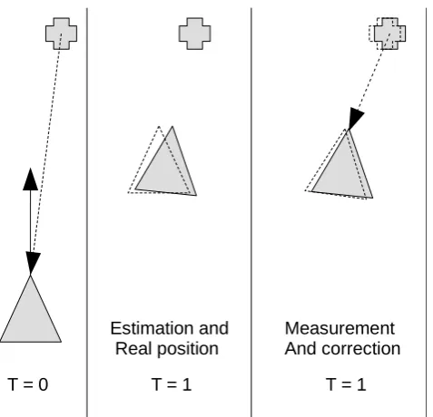
SLAM, as the name implies is a family of algorithms to simultaneously map an environment, and use this map for correction the own position. Most of this algorithms are based on prob-abilistic models of the position and the environment. The output will then be the most likely, according to the algorithm, position and environment. The SLAM algorithm consists of two major parts: a prediction step and a update step. In the predict step the internal information of the robot, for example control signals, odometry or an IMU, is used to predict the new state of the robot. In the update step external information is used, usually measurements of the envi-ronment, to correct the prediction of the robot and the environment. A schematic overview of this behaviour is shown in Figure 2.1. It is important to note that not only is the robot position corrected, but that the estimation of the landmark is also corrected with the measurement.

2.1.1 Statistical model

The prediction step of the SLAM algorithm can be mathematically expressed as:

p(x�_t|ct,xt₋1)

Withxthe state of the system, andcthe control signals. This probability includes disturbances based on the system noise. As the period over which the state is predicted become larger it becomes less accurate, as is shown in Figure 2.2. The prediction that is started earlier has a larger error then the later prediction.

The update step of the SLAM algorithm can be expressed mathematically as:

p(xt|x�t,zt)

Withx�_{the corrected state and}_z_{the measurement of the environment. The state of the system}

also includes the landmark positions. This is shown in Figure 2.1, where the position of the landmark is also estimated. Both the update step and the predict step use information that will contain uncertainties. By combining this information in an intelligent way, theﬁnal estimation of the state can be more accurate then a single measurement/prediction could provide.

2.1.2 Feature detection

In the previous section landmarks are mentioned, but usually the environment has no clearly deﬁned landmarks. This is where the feature detector comes in. The feature detector takes raw data from the environment and extract features from this data. This process is shown in Figure 2.3.

(10)

T = 0 T = 1 Estimation and Real position

[image:10.595.167.406.82.312.2]

T = 1 Measurement And correction

Figure 2.1:A SLAM system in action. The robot (triangle) measures the landmark (plus), moves forward and measures the landmark a second time, correcting its estimation of its own position and that of the landmark.

[image:10.595.78.494.378.552.2]

Robot path Prediction 1 Prediction 2

Figure 2.2:A prediction of a robot driving forward with some motion noise. Prediction 1, which is started earlier then prediction 2 has a larger error, while prediction 2 is much more accurate. The ellipses are a representation of the uncertainty of the position.

Laser scanner Feature detector

Features: 1: pos: …. 2: pos: ….

[image:10.595.120.453.614.735.2]

(11)

CHAPTER 2. BACKGROUND 5

[image:11.595.126.477.76.206.2]

Map layer Feature layer Complete map

Figure 2.4: The different layers of a map. In this situation the map is a 2D occupancy map, and the features are detected based on corners.

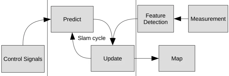
Update Predict

Control Signals

Measurement Feature

Detection

Map Slam cycle

Figure 2.5:A overview of the slam algorithm with a SLAM cycle (predict->update->predict).

2.1.3 SLAMﬁlters

The most important part of a SLAM system is the SLAMﬁlter, this is the algorithm that actually implements the predict and the update step. The result is only an approximation of the proba-bility density functions, as the true probaproba-bility distribution is to computationally expensive to be calculated. A multitude of differentﬁlters exist to implement this approximation. More on this is shown in Section 2.2.2.

2.1.4 Maps

Another part of the system is to create a map of the environment. The environment is usually mapped in two layers when using a SLAM algorithm. The feature layer contains the features that are detected. This part is mostly used by the slamﬁlter for positioning. The map layer contains the "raw" data from the sensors, providing a physical map of the environment. This is shown in Figure 2.4.

2.1.5 Recap

An overview of the complete slam cycle is shown in Figure 2.5. In thisﬁgure it is shown that the SLAM cycle requires odometry data or control signals for the predict step, and features for the update step. The slam system results in a current estimation of the map every with every iteration of the slam cycle.

2.2 The current state of SLAM

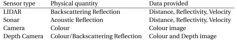
[image:11.595.103.499.256.388.2]

(12)

Sensor type Physical quantity Data provided

LIDAR Backscattering Reflection Distance, Reflectivity, Velocity Sonar Acoustic Reflection Distance, Reflectivity, Velocity

Camera Colour Colour image

[image:12.595.91.483.80.150.2]

Depth Camera Colour/Backscattering Reﬂection Colour and Depth image

Table 2.1:The different types of sensors, including physical quantity and the type of data provided

discussed. Secondly the different families of algorithms and their strong and weak points are discussed.

2.2.1 Sensor Types

The sensors that are used the most in SLAM systems can roughly be divided into 4 sets of sen-sors. Both based on the physical quantity that the sensor measurement is based on, and the type of data that the sensor provides. These four sets are:

• LIDAR, 1D,2D and 3D. (Kohlbrecher et al., 2011; Li and Olson, 2010)

• Sonar, both 1D and 2D (Choit and Ahnt, 2005; Ribas et al., 2006)

• Camera, both Intensity and RGB (Davison et al., 2007; Steder and Grisetti, 2008)

• Depth camera, both depth and RGBD (Sturm et al., 2012; Endres et al., 2012)

The different physical quantities and data types of these sensors are shown in Table 2.1. It is important to note that depending on the exact sensor conﬁguration, the data that is returned can be a 1D, 2D or 3D.

Based on this table, it can be deduced that different types of sensors may have problems de-tecting different kinds of obstacles. A simple example is a mirror or glass plate, a camera or LIDAR will be confused by the reﬂections or the transparency, while a sonar based system has a much better change of detecting this correctly. The sonar will however have trouble with sound absorbing material, which is not a problem for the optical systems, unless the material is also light absorbing.

Another limitation for sensors is the effective range. While a LIDAR system can measure dis-tances up to, and exceeding 30m (Hokuyo, 2012), sonar systems can only measure upto a cou-ple of meters with any speed (MaxBotics, 2005), and camera systems can go up to near inﬁnite ranges, limited only by visibility. These limitations are imposed by the difference in the speed of sound and light in air, and will be different in other media e.g. water.

2.2.2 Algorithm Families

The algorithms used in a SLAM system in general consist of two parts. First the feature detec-tion, which transforms the sensor data into feature locations. Secondly a probabilistic algo-rithm which uses this pose estimation to improve the world belief. Both are discussed here.

Feature detection

Feature detection simpliﬁes the sensor data into features which can be easily associated and stored. One can also use the complete measurement using a scan matching approach, but this takes a signiﬁcantly larger amount of computational resources (Li and Olson, 2010).

(13)

CHAPTER 2. BACKGROUND 7

Sensor type Computational complexity Flexibility

Scan matching High High

(Li and Olson, 2010)

Attention-based F.D. Medium Medium

(Vu et al., 2007; Li and Olson, 2010)

Fixed F.D. Low Low

(Gil et al., 2009; Choit and Ahnt, 2005; Kim and Oh, 2007)

Table 2.2:The different types of feature detection/matching, including the computational complexity and theﬂexibility

about the environment and thus performs badly when these assumptions are false. E.g. while using a system optimized for line and corner detection will perform poorly in a park in contrast to inside a building.

Another option is to use a feature detection algorithm based on attention. This evaluate the

ﬁtness of landmarks based on the contrast with the environment. So instead of looking for a

fixed structure, it will detect whatever aspect of the environment gets the most attention. This results in a moreflexible feature detector (Vu et al., 2007; Li and Olson, 2010). An overview of these options is shown in Table 2.2, with a comparison of computational complexity, and how well the algorithm deals with different environments, i.e. theflexibility.

From this table it can be concluded that the moreﬂexibility is necessary for a system, the higher the computational costs. There are also hybrid solutions, which mitigate this effect by, for ex-ample, using both a line and a corner detector for feature recognition, but as more different detectors are added to a system, it quickly approaches an attention-based approach.

Processing Algorithm

There are different ways of processing the feature measurement in order to obtain position in-formation. It can be done using different algorithms, The biggest split is the use of Bayesian techniques, where the features are used to refine a prior estimation of the position in order to improve the current estimate, or using direct position estimation, where the feature informa-tion isfirst used to estimate the robot position directly before that position is used to update the position estimation. Bayesian techniques can then be implemented using Extended (Civera et al., 2008; Cole and Newman, 2006; Artieda et al., 2009; Choit and Ahnt, 2005; Davison et al., 2007) or Unscented Kalman (Chekhlov et al., 2007)filters or by using particlefiltering (Grisetti, 2005). Direct pose estimation is most easily done using visual slam, combined with for exam-ple RANSAC (Endres et al., 2012; Artieda et al., 2009; Steder and Grisetti, 2008) or otherfitting algorithms. All of these different algorithms benefit from using a smoothing or optimization algorithm for loop closing problems (Kohlbrecher et al., 2011; Frintrop et al., 2006; Steder and Grisetti, 2008; Se et al., 2005), for example g2o (Endres et al., 2012).

The more linear estimations algorithms, especially the Kalman filters, have problems rep-resenting multi-modal beliefs (Thrun, 2002), thus these algorithms, while computationally cheaper, perform badly in global localization cases, for example the kidnapped robot prob-lem1. In contrast, particlefiltering and direct pose estimation perform significantly better, at significantly higher costs.

All of theseﬁlters are in essence suitable for a global and local localization problem, however as the amount of poses remembered grows it might be useful to prune the information. This is

(14)

(15)

9

3 Analysis

In order to reduce deployment time and development time, it is important to be able to reuse as much of the existing system as possible. To accomplish this, it is important to analyse how the different parts can be reused. Depending on, in what situations different parts of the system can be reused, it can be determined which parts of the system can be implemented in the same module.

Furthermore, this chapter contains a section on using multiple robots, which could be possible due to standardisation, and on correction done between robots. In Chapter 4 a solution to some of the problems found in this chapter is proposed.

3.1 Reusability

To be able to reuse any part of the system implies that the system isflexible enough to function even when assumptions on which it is based are changed. This means it should be able to con-tinue functioning with minimal changes, or at least with most parts of it intact. In order to be able to design a system like this, it is important to define the different changes that can hap-pen. This allows the system to be designed in such a way that a single change only influences a single part of the system.

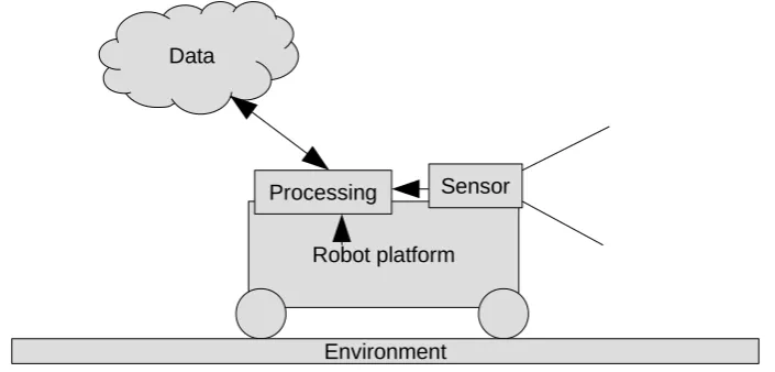
A schematic overview of a working SLAM system is shown in Figure 3.1. The different changes that can be made can be split as follows. The effects of the different changes are discussed in more depth in the following subsections. These three option only reﬂect the reuse of the system on a possibly different platform. The other option of reuse is that the data that is acquired by one robot is reused by another robot.

• The robot platform changes, thus changing kinematics of the robot.

• The sensor changes, thus requiring a different system to process sensor information.

• The environment changes such that a different state estimation algorithm is needed.

• The data is reused on a different robot.

The fact that data can be reused by different robots could also be exploited to allow multiple robots to work in parallel on a single map. This is not a trivial problem, as more care needs to

Data

Robot platform Sensor Processing

[image:15.595.126.479.571.740.2]

Environment

(16)

[image:16.595.104.470.78.251.2]

Diffential drive Ackerman steering Holonomic drive

Figure 3.2:Different modes of steering for a robot

be taken to be able to correctly correlate the data real-time. This requires a way to determine which robot is right in the case of conﬂict.

The system can be made mostly reusable if one of the parts can be swapped without inﬂuencing the other parts. Making the SLAM system as reusable as possible.

3.1.1 Reusing on a different robot platform

Changing the hardware of the robot can mean two different things:

1. The processing hardware of the robot is changed.

2. The physical structure of the robot is changed.

The assumption is made that theﬁrst part can be solved by using modern compilers/software stacks. This analysis only focusses on the second option. When the hardware of the robot changes the kinematic model of the robot also changes. This can only be a parametric change (e.g. larger wheels), or can be a change to the type of model. For example a differential drive is changed to Ackerman steering or a holonomic drive. An example of these differences is shown in Figure 3.2 As the kinematic model of the robot only deals with the localization, it does not need to take into account other states of the robot. The assumption is made here that the state of, for example, a manipulator on top of the robot has a minimal inﬂuence on the location of the robot itself.

In order to be able to contain not only the changes in parameters but also in changes of the motion model, the whole kinematic model of the robot should be self contained. Thus the model contains all parameters relevant to predicting the robot movement from a previous state and a control signal.

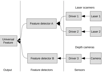
3.1.2 Using different sensors

A different sensors can change the requirements of the system that is processing the sensor data in two ways:

1. An other driver is needed to interpret the sensor data.

2. An other way of processing the sensor data into features is needed.

(17)

CHAPTER 3. ANALYSIS 11

Feature detectors Sensors

Laser 1

Laser 2

Camera Driver 2

Driver 1

Driver 3

Laser scanners

Depth cameras Feature detector A

Feature detector B Universal

Feature

[image:17.595.124.484.77.329.2]

Output

Figure 3.3:Different sensors require different drivers and possibly different feature detectors, but in the end the output is the same.

scanner, then there is no need to change the feature detection, but depending on the format that of the output of the sensor driver, a translation step might be necessary. If one would change from a laser scanner to a depth camera, a signiﬁcantly different feature detector might be necessary. This situation is shown in Figure 3.3

The features that are supplied by a feature detector should be in an universal format. This allows the rest of the system to remain the same. This requires all information needed to change the raw sensor data to something that is processable by the robot to be contained in the sensor module. This includes sensor positioning, but also uncertainty information.

3.1.3 Using various state estimation algorithms

The various algorithms used for state estimation take advantage of the standardization of the feature detector and the kinematic model. This means that all algorithms have to estimate the same state, a 6 degrees-of-freedom pose. The choice for a 6DOF pose was made because a 6DOF pose allows a representation of a 3DOF pose by simply assuming the other three to be constant, but the other way around is not possible.

Depending on the kinematic model and feature detector it might also be impossible to estimate all 6 degrees of freedom, which then must be assumed unknown or constant. It is also assumed that derivatives of the pose (velocity and acceleration) will be provided by odometry data or other sensors. The algorithms are designed in such a way that as much information about the localization as possible is stored in the map, instead of in the algorithm itself. This will allow most of the data to be reused when an algorithm is swapped out. However as the map cannot change in implementation when the algorithm changes, it is probably necessary to save some algorithm-speciﬁc information in the algorithm instead of in the map.

3.1.4 Reuse SLAM Data

(18)

to be used in later expeditions into the same environment. If the data acquired is to be used to successfully navigate in an environment, it is necessary to at least store occupancy data. It could also be useful to store 3D coloured maps to allow human visualization of the data. In order to be able to use the mapping data for another algorithm it is important that the features that are detected are saved. Not only is their position needed, but also the feature descriptor and the uncertainty information. This means the map has to contain:

• Occupancy map

• 3D color map

• Features

– location

– descriptor

– uncertainty

The occupancy map and 3D color map, might not be both used, depending on the types of sensors available to the robot. As the map needs to be usable by multiple robots it is important to allow multiple algorithms to access the map data independently. Based on the size of the map, it should also be possible to only load a part of all the data. In this way a robot will not need to be able to process the whole map. It is important that the map can contain as much probabilistic information as possible without growing unnecessary large and in a format that is compatible with as much different algorithms as possible.

3.2 Multiple Concurrent Robots

If the SLAM system is structured in such a way that the map information and the position esti-mation algorithm are independent of one another it would be possible to have multiple robots or actors active at the same time. These actors could then map an area cooperatively.

Care has to be taken that the algorithms used are able to handle outside changes and that the map is not treated as a place to write data to, but that the map is also read for changes by the other robot. The position estimation algorithms would have to actively read back their information from the map.

Another obstacle to multiple actors is the relative localization between actors. This is not a problem if the actors start in known relation to one another, but if the actors are started in-dependently, it might cause problems. This is especially the case when feature detectors are used that cannot discern between different features, as then there is no way to correlate the positions of the different actors.

3.3 Correction using data

(19)

CHAPTER 3. ANALYSIS 13

Sensor system

Kinematic Model Sensor

Driver

SLAM Algorithm

Feature Detector

[image:19.595.105.502.81.186.2]

Map Storage

Figure 3.4:A SLAM system with a single robot

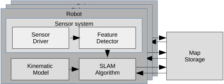
Robot Robot Robot Sensor system

Kinematic Model Sensor

Driver

SLAM Algorithm

Feature Detector

Map Storage

Figure 3.5:A SLAM system with multiple robots

3.4 Overview

[image:19.595.110.493.219.362.2]

(20)

4 Architecture

In this chapter, the focus on the design of the architecture of reusable SLAM systems. This design is based on the problem context mentioned in Chapter 3 and poses a general solution for the system. A implementation of this architecture is discussed in Chapter 5. The structure from Chapter 3 isﬁrst split up further and structured based on the dependencies of the different parts. Then the interfaces between the different parts are discussed. Finally the global structure of the system are discussed including the requirements of the implemented system.

4.1 Dependency of structure

The structure given in Figure 3.4 is further analysed by determining which parts needs to change when the underlying robot or the environment changes. This allows for clear bound-aries to be drawn between parts of the system based on how speciﬁc a part is for a certain situation. This allows the different parts of the SLAM system to be divided into:

• Robot speciﬁc

• Sensor speciﬁc

• Feature speciﬁc

• Environment speciﬁc

• World speciﬁc

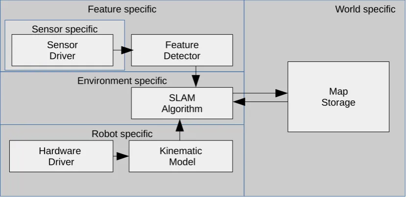
The resulting structure is shown in Figure 4.1. This structure deﬁnes four clean boundaries in the system. These are discussed in the next section.

4.2 Interface between blocks

The structure of Figure 4.1 deﬁnes a few clear boundaries between subsystems. These bound-aries are between:

• The feature detector and the SLAM algorithm.

• The kinematic model and the SLAM algorithm.

• The SLAM algorithm and the map storage.

• The sensor driver and the feature detector.

In this section these interfaces will be speciﬁed, based on:

• What information needs to pass through the interface.

• How this information is represented.

• In what direction this informationﬂows.

Based on these criteria the different interfaces will be speciﬁed in the following subsections

4.2.1 SLAM algorithm to map storage

(21)

[image:21.595.94.513.80.283.2]

CHAPTER 4. ARCHITECTURE 15 Environment specific Feature specific Robot specific Kinematic Model Sensor specific Sensor Driver SLAM Algorithm Feature Detector World specific Map Storage Hardware Driver

Figure 4.1:A SLAM with the dependencies of the different subsystems.

data that is directly read from the map by the SLAM algorithm are the features. These three different data types are represented differently. The occupancy map is written by using scan data to indicate free/occupied terrain. This means the input should be a local occupancy map. The color map needs 3D color information, preferably as a point cloud, which can then be included in the map. Both of these data types are dependent on the location of the actor, thus the position estimation of the SLAM algorithm needs to be available as well. The data that is written to the map will have to be processed in order to be able to include it. As a occupancy map can have a certain uncertainty as can a 3D map. The features consist of: a location, a descriptor and an uncertainty region. All this data needs to be available with the feature. It is critically important that the covariance between features can also be represented while sending this data to the map. Thus theﬁnal interface consists of three parts:

• Occupancy data (SLAM to map)

– 2D Occupancy data

– robot pose estimation

• Colour map (SLAM to map)

– 3D point cloud

– robot pose estimation

• List of features (bidirectional)

– Poses

– Descriptors

– Covariance matrix

Note that the occupancy and 3D information still need to be accessible for software dealing with path-planning or map creation, but is just not used by the SLAM algorithm.

4.2.2 Kinematics to SLAM algorithm

(22)

The kinematics interface can return this transformed state in three different ways. This will allow different algorithms to function using the kinematic model:

• A direct deterministic estimation of the state.

• A direct estimation with an uncertainty region.

• A sample from the uncertainty region.

The direct estimation can be used in for example an Unscented Kalman Filter (UKF) The esti-mation with an uncertainty region can be used for a system which uses a linear estimator, for example a Extended Kalman Filter (EKF). The Sample estimation can be used for systems using particleﬁlters.

All three of these options will require a state vector and a time period to function. Thus the interfaces can be described as:

• input (SLAM to model)

– State vector

– Time period

– Depending on the type:

* Covariance matrix

• output (model to SLAM)

– State vector

– Depending on the type:

* Covariance matrix

It is important to note that the kinematic model also includes the probabilistic information of the robot hardware. This means that all effects of control signals or errors are modelled in the kinematic model. The slam algorithm will no need any information on the speciﬁcs of the hardware platform.

4.2.3 Feature detector to SLAM algorithm

The feature detector needs to supply positional and uncertainty information about the features that it detects. In order to be able to match the detected features, it is also important to know the type of feature that is detected and the descriptor of the speciﬁc feature. This information is only written to the SLAM algorithm. The features are represented as a list of:

• Poses

• Uncertainty regions

• Descriptors

• The types of the features

4.2.4 Sensor to feature detector

(23)

CHAPTER 4. ARCHITECTURE 17

4.3 Structure

Based on the previous section, a reusable andﬂexible SLAM system consists of the following components:

• Self contained sensor module, including probabilistic functions

• A kinematic model of the robot including odometry data

• Feature detector working on sensor data

• A universal standard for storing features, world belief and pose history

• A pose estimator based on standardized world belief and features

• Map Smoothing algorithms working on universal world belief

A complete SLAM system would then have the structure as represented in Figure 3.4. However as these different parts are independent of each other, they can be used in parallel, allowing multiple sensors, feature detectors, pose estimators or even multiple robots working on the same world belief. This is represented in Figure 3.5. This means that the world structure will have to be set up in such a way that it can handle multiple systems working on it at the same time. As the inputs of the system (odometry,sensors) can be supplied at different rates, a choice is made to use the sensors, and by extension the feature detector, as a determining factor for the timing of the system. This means that the odometry data will have to be synchronized to the sensor data.

4.4 Design targets

As this project was limited in time the requirements from Chapter 3 and Chapter 4 are divided into four categories. This is done according to the MoSCoW principle. Thus they are divided intomust,should,couldandwill not. This division is shown in Table 4.1

Must Should Could Will not

Single implementation of interfaces SLAM validation Map validation Multiple robots

A SLAM algorithm Map smoothing reuse validation

A feature detector Corrections based on data

A kinematic model A map

Table 4.1:MoSCoW requirements for this project

The Single implementation of interfacesmustentail the creation of hard deﬁnitions of all the interfaces in a format that can be directly synthesized into code. Based on these interface a modulemust be implemented for a SLAM algorithm, a feature detector, a Kinematic model and a map. If possible the SLAM algorithmshouldbe validated based on a existing dataset. If possible a algorithmshouldbe created to smooth the map.

If a large map can be created thiscouldbe used to validate the creation of such a map using a existing dataset.

The suggestions mentioned in Chapter 3 for multiple actors, and correction based on big data

(24)

5 Implementation

There is a multitude of systems available for implementing robotics software, but for this project ROS indigo (ROS, 2014) has been chosen as software platform. This because the ROS platform allows nice separation of the different blocks by using nodes, and ROS requires hard deﬁnitions of interfaces and topics. These exact deﬁnitions used can be found in Appendix A. Using ROS, a single implementation of this SLAM system is made. This does not validate the re-usability criterion, but shows that the structure is valid for SLAM.

This chapterfirst shows the hardware used for the project and then continues to the imple-mentation of the different subsystems as explained in Chapter 4 All specification of interfaces and algorithms are described in a single package. The robot and sensor-specific elements are created in separate packages. This results in the structure as shown in Figure 4.1.

5.1 Hardware

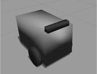
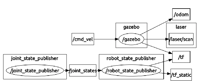
[image:24.595.114.455.400.660.2]

As the goal of this project is to create the architecture for a reusable SLAM system, and not to implement SLAM on a speciﬁc robot. the choice was made tonottest on real hardware, but use a simulation of a robot by using Gazebo(gaz, 2016). This allows quicker testing and allows the project to be completely self-contained. The simulated robot is build, based on a platform with a differential drive. This allows easy navigation and control. The dimensions of the robot are chosen small enough (60x45x40cm) so that it can easilyﬁt a door-frame or navigate in small spaces. The robot model is shown in Figure 5.1

Figure 5.1:The simulated model of the robot in Gazebo (gaz, 2016). The black bar on top represents the laser scanner.

(25)

[image:25.595.126.472.83.225.2]

CHAPTER 5. IMPLEMENTATION 19

Figure 5.2:The ROS structure in which Gazebo publishes the robot state and sensor measurements. The /t f topic is used by ROS to publish transforms between coördinate frames

also published the state of the robot joints. The full publishing structure of the Gazebo model is shown if Figure 5.2. As this project does not include any form of navigation, the robot is driven around manually for measurements.

5.2 Feature detection

As the simulated robot has a laser scanner, a feature detector that works on laser scan data is required. The technique described by Li and Olson (2010) is used to implement this. This technique allows general purpose LIDAR features to be extracted from data. It does this byfirst mapping laser data to a 2 dimensional image, before applying image processing techniques tofind features. The important technique is to map the laser data onto an image in such a way that the information that the laser scan represents is kept in the image. A few design de-cisions, required for the implementation of the feature detector, were not specified in Li and Olson (2010). These decisions are the segmentation of data and the handling of occlusion. The segmentation was handled based on a distance threshold between two points. The occlusion was handled by identifying occluded points and excluding the region around this point from feature detections. Both of these parameters were left configurable, in order to determine an optimum. The general process of the feature detector is shown in Figure 5.3.

Laserscan data segmentation extrapolation

filtering Occlusion masking

Feature detection

Figure 5.3:The processing chain for the feature detector. The circles indicate regions in which features are rejected. The crosses indicate detected features.

[image:25.595.115.488.519.686.2]

(26)

Buffer

Odometry Tim

e Transform request

From (Time)To (Time) State[]

Response _{To SLAM algorithm}

State[]

From SLAM algorithm

[image:26.595.81.488.81.252.2]

Covariance[] Covariance[]

Figure 5.4:The implementation of the kinematic model as the transformation of a state. The buffer is

ﬁlled at aﬁxed frequency and buffers a certain amount of time. The state is transformed from theFr om

time to theTotime.

5.3 Kinematic model

The raw odometry is provided by Gazebo at aﬁxed frequency. This frequency is not the same as the frequency of the laser scanner or the SLAM algorithm. This means the odometry data needs to be saved in a buffer to be applied to a state when required. So when for example the odometry data is published with 100Hz and the sensor data is only provided at 10Hz, 10 odometry messages are needed for every predict step. The kinematic model provides a few services to transform a state, but all the different services have in common that they have a

f r omand atotime. So that a prediction can be made over a arbitrary time frame. These times can then be looked up from the buffer to allow a state transformation over all the odometry data received in this time frame. This process is shown in Figure 5.4.

As mentioned in Section 4.2.2 the kinematics model should return three different estimations: A direct estimation, a estimation with an uncertainty region and a sample from the uncertainty region. All three options are implemented as different services and are shown in Appendix A

5.4 SLAM Algorithm

(27)

CHAPTER 5. IMPLEMENTATION 21

Partic lePar ticleFor every Particle

Detected Feature Detected

Feature DetectedDetected

feature

Distance to known features

Update known feature < X

Ignore measurement > X < Y

Create new feature

> Y For every ParticleFor every ParticleFor every Particle

Update State with kinematic model Wait until new

measurement

Weigh particles Resample

[image:27.595.106.502.226.576.2]

particles Start

(28)

5.5 World speciﬁc

(29)

23

6 Experiments

The design posed in Chapter 4 is implemented in ROS. The information about the code repos-itory is shown in Appendix B. Based on this reposrepos-itory a set of tests are executed to asses the performance of the different parts. As some of the modules are implemented using ROS pack-ages, they are not explicitly tested. These parts are the simulation model, the map and the drivers. This means that the feature detector, the kinematic model and the Fast-SLAM algo-rithm are tested. Theﬁrst test only tests the feature detector. The second test also includes the kinematic model and the Fast-SLAM algorithm.

6.1 Feature detector

The Feature detector is tested by simulating the robot in a structured environment. The envi-ronment that was chosen was the willowgarage model as is provided by Gazebo. This environ-ment is shown in Figure 6.1. Based on this environenviron-ment the parameters shown in Listing B.1 are changed and evaluated. These parameters are divided into different sections:

• Image resolution

• Laser Properties

• Segmentation

• Feature detection

These different sections are discussed separately.

6.1.1 Test method

To test the effect of the different parameters the feature detector was started using the instruc-tion from Appendix B. This loads the parameters from the conﬁguration. The set of parameters was then evaluated based on the following criteria:

• Features are detected on some corners in the environment.

• There are no features in empty space.

• There are no features on straight sections of wall.

During the development of the system the values were selected to produce at least a working system. In order to explore the boundaries of the working parameters, the parameters were then changed pseudo-randomly and the situations, which led to problems were found using trial and error. The effects of the different parameters are described in the following sections.

6.1.2 Image resolution

The image resolution section of the conﬁguration contains three settings: Thepixels-per-meter

(ppm), thekernel radiusand thescale levels.

Theppmindicated how many pixels are in a meter at the smallest scale level. Increasing this value increases computation time quadratically as all images increase in size. When this value is made very small it becomes difﬁcult for features to be detected accurately, but this only hap-pens in the region of 10 pixels per meter.

(30)

[image:30.595.72.499.240.583.2]

(31)

CHAPTER 6. EXPERIMENTS 25

Actual Structure

Too much seperation

[image:31.595.135.471.78.236.2]

Too little seperation

Figure 6.2:The problems of too much or too little segmentation. In both cases more features (crosses) are detected then in the ideal situation. The circle is the sensor position.

enough to contain the actual kernel, however increasing the size also increases the computa-tional load by a signiﬁcant amount.

Thescale levelsdetermine the amount of different scales used in the feature detection algo-rithm. As mentioned in Li and Olson (2010), the feature detection algorithm is scale invariant because the images generated from the laser data are downsampled. When this parameter is set too large, the resolution of the lower scale images approaches resolutions that are no longer sensible, in the order of 10-1 pixels-per-meter. The consequence of this is that random features are detected in regions that are nowhere near actual features. This is off course dependent on the feature size of the environment.

The parameter ranges in which the feature detector works are present in Table 6.1.

6.1.3 Laser Properties

The laser properties conﬁguration are based on the model of laser-scanner used and are shown in Table 6.1. Thelaser range sigmais the standard deviation of the range error made by the laser scanner, and thelaser angle sigmais the standard deviation of the angle error made by the laser scanner. These parameters are used to determine the kernel size of the smoothing algorithm. There is no limit on these parameters, but a laser scanner with higher standard deviation will perform worse.

6.1.4 Segmentation

The Segmentation section of the conﬁguration contains three parameters, thedistance thresh-old, theocclude limitand theextrapolation distance

Thedistance thresholdproperty is used for segmenting the laser-scanner data. When this value is chosen too small, continues structures will be treated as different sections. This results in a ’break’ in the structure, and causes features on the ’break’. This means the value should always be larger then the expected distance between measured values. When the value becomes too large, different structures are treated as a single structure. This will remove certain features, and create false features due to occlusion. This effect is shown in Figure 6.2.

(32)

Theextrapolation distanceshould be large enough that even at the lowest scale levels, the edge of the extrapolation is far enough away from the corner to not inﬂuence the feature. It can be arbitrary large, but this will increase computational costs.

See Table 6.1 for the actual parameters used.

6.1.5 Feature Detection

The feature detection section contains the parameters used for the corner detector which is used in the feature detector. The parameters for the corner detector are themax features, the

feature threshold, thefeature distanceand thecovariance limit.

Themax featuresdetermines the maximum amount of features that a the feature detector can detect in one segment. When this is set too low there is a possibility that all detected features are rejected. Setting this too high will increase computational time, but this is limited by the other parameters.

Thefeature thresholdlimits the quality of features. This setting determines the minimum qual-ity of a feature based on a factor of the best feature. This parameter suffers the same problem as the max features. When it is set too strict (above 0.95), it is possible that all detected features are invalidated due to other reasons, resulting in no detected features. Setting it too low, will result in a lot of low-quality features, which might be false positives.

Thefeature distanceoption sets the minimum distance between detected features. If this is set too small, multiple features are detected in the same corner. When this happens is very dependent on the environment. It can be set very large, but this increases the risk of all features being rejected. Just as the previous settings.

Thecovariance limit is a limit based on the covariance matrix of the feature. The feature is rejected if one of the covariances is larger then this limit. Just as the previous limits, care should be taken that this is not too strict (too small), as then there is a possibility that all features are rejected.

Theﬁnal parameters used are shown in Table 6.1.

6.1.6 Final results

Based on the selected parameters a test is run. The testing situation is shown in Figure 6.3. The result of the feature detector is this situation is shown in Figure 6.4. The large circles are the regions that are excluded from feature detection due to the occlusion or projection. The small ellipses are the detected features with their 1σuncertainty regions. From this image it can be seen that features are only detected on "real" corners. There are no false features provided due to occlusion or by the projections of the laser scanner.

6.1.7 Discussion

The feature detector has some problems with detecting false features in straight sections of wall. The computational costs can also become quite high when certain parameters are in-creased. Especially image resolution.

Overall features are detected well, but large unbroken sections can have the result that a single ’good’ feature can obscure a few more subtle features, but as soon as the ’good’ feature is no longer observed the others are valid.

6.2 SLAM algorithm

(33)

[image:33.595.112.494.90.375.2]

CHAPTER 6. EXPERIMENTS 27

Figure 6.3: The environment the robot is tested in. The result from the feature detector is shown in Figure 6.4

[image:33.595.144.475.450.688.2]

(34)

Parameter Minimum Used Maximum Image resolution

ppm (pixels) 50 100 200

kernel radius (pixels) 15 40 100

scale levels 1 3 3

Laser Properties

laser range sigma (m) - 0.02

-laser angle sigma (rad) - 0.0036 -Segmentation

Distance threshold (m) 0.3 0.3 1

Occlude limit (m) 0.3 0.03

-Extrapolation distance (m) 1 1

-Feature Detection

Max features 5 10

-Feature limit 0.7 0.9 0.95

Feature distance (m) 0.15 0.3

-Covariance limit - 0.7

-Table 6.1:The range of parameters which gave acceptable results for the feature detector and theﬁnal values chosen. These are only approximate values for good performance, not absolute limits, and are dependent on the environment. ’-’ means no limit was found.

These tests are done by manually driving the robot around in the testing environment and assessing the performance.

6.2.1 Test Method

The Fast-SLAM algorithm is tested in much the same way as the feature detector. The system is started according to Appendix B and the evaluation is done based on the criteria:

• The position did not drift away.

• No extra landmarks are created when driving the robot a bit.

• No landmarks are created in empty space.

• When a complete circuit of the room was made, the landmarks were re-discovered.

Working parameters were selected during development and were varied pseudo-randomly in order toﬁnd parameter conﬁgurations that would cause problems. The effects of these param-eters are described in the following section.

6.2.2 Parameters

The Fast-SLAM algorithm has 4 parameters. Three of these parameters,particle amount, fea-ture match distanceandminimum feature separationaffect the functioning of theﬁlter directly.

future interpolaffects the ROS framework.

The particle amount option sets the amount of particles used in theﬁlter. Increasing this should result in more accurate representation of the probability density functions, with a in-crease in computational cost. A minimum of about 50 particles is advised, but there is no max-imum limit.

[image:34.595.140.433.79.323.2]

(35)

fea-CHAPTER 6. EXPERIMENTS 29

Parameter Minimum Used Maximum

Image resolution

particle amount 50 100

-feature match distance 0.1 0.1

-minimum feature separation 0.3 0.3

-future interpol(s) 0 0.1

[image:35.595.155.450.79.165.2]

-Table 6.2:The range of parameters which gave acceptable results for the Fast-SLAM and theﬁnal values chosen. These are only approximate values for good performance, not absolute limits, and are depen-dent on the environment and the settings for the feature detector. ’-’ means no limit was found.

Figure 6.5:A small bit of the map generated. The white dots are detected features. The light grey areas are passable and the black areas are impassable. The dark grey is unknown.

ture separationare too small, features will not be associated after a bit of drift. If it is too large, features will be associated with the wrong features. This is highly dependant on the feature spacing of the environment and on the conﬁguration of the feature detector. There was not really an optimal value for these parameters.

Thefuture interpolsetting determines how long the position published by the Fast-SLAM node will be considered valid. Setting this too large will results in other nodes working with old data. Setting this too small might result in the fact that there is no valid prediction for the present if the delays of the feature detection and the Fast-SLAM algorithm are too big. The ideal setting for this parameter is very dependant on the rest of the system.

6.2.3 Final results

[image:35.595.91.519.217.508.2]

(36)

6.2.4 Discussion

A problem that was quickly noted in this system is that there are a few features that are appar-ently in free space. This is caused by problems in matching features with new measurements, as the distance to match features was too small to correct for the drift of the robot. This distance could not be increased as there were features in the environment that were close together. This posed a problem for validation as the algorithm was not stable enough to map the whole dataset provided. Thus there are no numerical results to compare to.

This association problem limits the efﬁciency of the algorithm, but also limits the possibilities of working together with multiple robots without extra coördination.

The feature detection could be improved by implementing a feature detector that has a (semi-) unique classiﬁer for every feature. Something based on (stereo-) vision. This should also eliminate the SLAM algorithm problems, as these were mostly based on feature matching. The current system has a few speed/time limitations, this is partially caused by the fact that the system was not optimized for performance in any way, and that a lot of debug information is still present.

(37)

31

7 Conclusion and Recommendations

Based on the experiments performed in Chapter 6, it can be concluded that the structure is working. This chapter discusses the functioning of the structure and how to improve it.

7.1 Conclusions

The current structure appears to be correct. However when one looks at the separation of con-cerns it is clear that the feature matching that is done by the SLAM algorithm right now, should be part of the feature module. Furthermore, the map interface is not clear enough yet, as the advanced parts of the map interface could not be implemented due to problems with the algo-rithm.

7.2 Recommendations

Theﬁrst recommendation for the structure is to separate the feature matching from the SLAM algorithm and move this to the feature detector package. This would also allow multiple feature detectors to be used in parallel.

The second recommendation of the structure is to test the interface between the SLAM algo-rithm and the map. As of right now it is not used very much. The re-usability of the structure has not been validated. This should be done by implementing the system on different hardware and with different sensors.

7.3 Future work

Based on this conclusion and on the discussion from Chapter 6 there are 3 steps that need to be taken to be able to use this system on a real platform.

• A feature detector with a (semi-) unique classiﬁer.

• A more advanced map.

• Enough performance optimization to run real-time.

A feature detector with a unique classiﬁer would solve the problem of feature association, which will make the Fast-SLAM algorithm more robust. It will also allow better coöperation between robots.

A more advanced map will allow better integration of probabilistic data into the map, which should also pave the way for multiple actors.

Performance optimization to allow the system should be possible. Especially if FPGAs or other specialized hardware is used to accelerate some parts of the system.

(38)

A Interface de

ﬁ

nitions

The interfaces used in the current system are deﬁned based on the ROS syntax for messages and services. In this appendix these deﬁnitions are sorted based on the module to which they belong. The rest of the interfaces currently use build in messages from ROS. Messages in ROS are structure by simply listing all elements of the message, for example:

✞ ☎

Header Header i n t a

i n t b

✝ ✆

Listing A.1:An example message deﬁnition.

is a message with a header, which contains things like the time of publishing and two integers: a and b.

A service includes the request parameters above the dashed line, and the response below, for example:

✞ ☎

i n t a i n t b

−−−

i n t sum

✝ ✆

Listing A.2:An example service deﬁnition.

is a service that takes two integers (a and b) in its request and returns a single integer (sum).

A.1 Kinematic Model

The kinematic model interfaces all contain a vector for the state (n elements) and possibly a second vector for the covariance (n×nelements). The output is again a state and possibly a covariance.

✞ ☎

fl oa t3 2[ ] s t a t e time from

time to

−−−

fl oa t3 2[ ] s t a t e

✝ ✆

Listing A.3:Service to directly update the state.

✞ ☎

fl oa t3 2[ ] s t a t e fl oa t3 2[ ] cov time from time to

−−−

f l oa t 3 2[ ] s t a t e f l oa t 3 2[ ] cov

✝ ✆

Listing A.4:Service to update the state including uncertainty information.

✞ ☎

f l oa t 3 2[ ] s t a t e time from

(39)

APPENDIX A. INTERFACE DEFINITIONS 33

−−−

fl oat3 2[ ] s t a t e

✝ ✆

Listing A.5:Service to update the state by taking a sample out of the uncertainty region.

A.2 Feature Detector

As stated in Chapter 4 the features require a pose with covariance, type and classiﬁer. This structure was implemented and a second message was deﬁned to publish a list of features

✞ ☎

Header Header s t r i n g type

s t r i n g c l a s s i f i e r

geometry_msgs/PoseWithCovariance pose

✝ ✆

Listing A.6:The message deﬁnition for a single feature.

✞ ☎

Header Header Feature[ ] Features

✝ ✆

(40)

B Repository Information

This is a modified version of the READMEfile supplied with the code project. This project con-sists out of multiple ROS packages for different responsibilities. All these packages are stored in a git repository. footnotehttps://git.ram.ewi.utwente.nl/R-SLAM The ROS modules include launchfiles to run certain systems.

B.1 Modules

The different modules are:

• ram_slamThe main module of the system, includes the message and service deﬁnitions as well as the SLAM algorithms

• ramscout_modelThis module contains the model of the simulated robot

• ramscout_kinematicsThis module contains the kinematic model of the robot

• ramscout_gazebo_pluginThis module contains all theﬁles required for the gazebo sim-ulation.

• ramscout_feature_detectorThis module contains the feature detector for use with the simulated robot.

B.2 Usage

To use this repository a few launchﬁles are provided. The two most important launchﬁles are:

ramscout_model/launch/RAMscout.launch

Which will launch the simulation of the robot.

ram_slam/launch/ramscout.launch

Which will launch not only the simulation of the robot, but will also start the feature detector and kinematic model.

ram_slam/launch/fast_slam.launch

Which will start the fast-slam algorithm

ram_slam/launch/map.launch

Which will start the map.

To start the complete system one would need to run

ram_slam/launch/ramscout.launch ram_slam/launch/fast_slam.launch ram_slam/launch/map.launch

(41)

APPENDIX B. REPOSITORY INFORMATION 35

B.3 Requirements

This system uses:

• Gazebo

• OpenCV2

Which need to be installed separately.

B.4 conﬁguration

There are 2 main configurationfiles used by the System. One for the feature detector, and one for the Fast-SLAM algorithm. The configurationfiles contain the following options

✞ ☎

#Image resolution

ppm: 100 # P i x e l s per meter , determines image resolution

kernel_radius : 40 # How large a kernel i s used for smoothing ( in p i x e l s )

s c a l e _ l e v e l s : 3 # The amount of scale l e v e l s for processing (1₋5)

#Laser Properties

laser_range_sigma : 0.02 # Stdev for the l a s e r range laser_angular_sigma : 0.0036 # Stdev for the l a s e r angle #Segmentation

distance_threshold : 0.3 # distance threshold for the segmentation .

occlude_limit : 0.3 # the minimum distance from occluded points a feature should be .

extrapolation_distance : 1.0 # How f a r the l a s e r corners need to be extrapolated , should be l a r g e r then occludelimit .

#Feature detection

max_features : 10 # Maximum amount of features to detect in a single segment .

feature_threshold : 0.9 # Feature quality l i m i t a l l features that are lower then t h i s f r a c t i o n of the best feature are discarded

feature_distance : 0.3 # Minimum distance between two features .

covariance_limit : 0.7 # Maximum covariance that a feature can have , before being rejected .

✝ ✆

Listing B.1:The conﬁguration of the feature detector

✞ ☎

particle_amount : 100 # Amount of p a r t i c l e s to use in a f i l t e r

feature_match_distance : 0.1 # Maximum distance that a feature can be associated

minimum_feature_seperation : 0.3 # Minimum distance required to create a new feature

future_interpol : 0.1 # Time in the future that a position estimation i s valid .

✝ ✆

(42)

Bibliography

(2014), ROS Indigo.

http://wiki.ros.org/indigo

(2016), Gazebo 7.1.

http://gazebosim.org

Artieda, J., J. M. Sebastian, P. Campoy, J. F. Correa, I. F. Mondragón, C. Martínez and M. Olivares (2009), Visual 3-D SLAM from UAVs,vol. 55, no.4-5, pp. 299–321, ISSN 0921-0296,

doi:10.1007/s10846-008-9304-8.

http://link.springer.com/10.1007/s10846-008-9304-8

Chekhlov, D., M. Pupilli, W. Mayol and A. Calway (2007), Robust Real-Time Visual SLAM Using Scale Prediction and Exemplar Based Feature Description,2007 IEEE Conference on

Computer Vision and Pattern Recognition, pp. 1–7, doi:10.1109/CVPR.2007.383026.

http://ieeexplore.ieee.org/lpdocs/epic03/wrapper.htm?arnumber= 4270051

Choit, J. and S. Ahnt (2005), Robust Sonar Feature Detection for the SLAM of Mobile Robot *. Civera, J., A. J. Davison and J. M. Mart (2008),vol. 24, no.5, pp. 932–945.

Cole, D. and P. Newman (2006), Using laser range data for 3D SLAM in outdoor environments, , no.May, pp. 1556–1563, doi:10.1109/ROBOT.2006.1641929.

Davison, A. J., I. D. Reid, N. D. Molton and O. Stasse (2007), MonoSLAM: real-time single camera SLAM.,vol. 29, no.6, pp. 1052–67, ISSN 0162-8828, doi:10.1109/TPAMI.2007.1049.

http://www.ncbi.nlm.nih.gov/pubmed/17431302

Endres, F., J. Hess, N. Engelhard, J. Sturm, D. Cremers and W. Burgard (2012), An evaluation of the RGB-D SLAM system,vol. 1, no.c, pp. 1691–1696, doi:10.1109/ICRA.2012.6225199.

Frintrop, S., P. Jensfelt and H. Christensen (2006), Attentional Landmark Selection for Visual SLAM,2006 IEEE/RSJ International Conference on Intelligent Robots and Systems, pp. 2582–2587, doi:10.1109/IROS.2006.281711.

Gil, A., O. M. Mozos, M. Ballesta and O. Reinoso (2009), A comparative evaluation of interest point detectors and local descriptors for visual SLAM,vol. 21, no.6, pp. 905–920, ISSN 0932-8092, doi:10.1007/s00138-009-0195-x.

http://link.springer.com/10.1007/s00138-009-0195-x

Grisetti, G. (2005), , no.April, pp. 32–37. Hokuyo (2012), UTM-30LX.

https://www.hokuyo-aut.jp/02sensor/07scanner/download/products/ utm-30lx/

Kerl, C., J. Sturm and D. Cremers (2013), Dense visual SLAM for RGB-D cameras,2013 IEEE/RSJ International Conference on Intelligent Robots and Systems, pp. 2100–2106,

doi:10.1109/IROS.2013.6696650.

(43)

Bibliography 37

Kim, S. and S.-Y. Oh (2007), SLAM in Indoor Environments using Omni-directional Vertical and Horizontal Line Features,vol. 51, no.1, pp. 31–43, ISSN 0921-0296,

doi:10.1007/s10846-007-9179-0.

http://link.springer.com/10.1007/s10846-007-9179-0

Kohlbrecher, S., O. von Stryk, J. Meyer and U. Klingauf (2011), Aﬂexible and scalable SLAM system with full 3D motion estimation,2011 IEEE International Symposium on Safety, Security, and Rescue Robotics, pp. 155–160, doi:10.1109/SSRR.2011.6106777.

Li, Y. and E. B. Olson (2010), Extracting general-purpose features from LIDAR data, inRobotics and Automation (ICRA), 2010 IEEE International Conference on, IEEE, pp. 1388–1393, ISBN 9781424450404.

MaxBotics (2005), XL-MaxSonar-EZ4.

http://www.maxbotix.com/Ultrasonic_Sensors/MB1240.htm

Montemerlo, M., S. Thrun, D. Koller, B. Wegbreit et al. (2002), FastSLAM: A factored solution to the simultaneous localization and mapping problem, inAaai/iaai, pp. 593–598.

Openslam (2016), Openslam.org.

http://openslam.org/

Ribas, D., P. Ridao, J. Neira and J. Tardos (2006), SLAM using an Imaging Sonar for Partially Structured Underwater Environments,2006 IEEE/RSJ International Conference on Intelligent Robots and Systems, pp. 5040–5045, doi:10.1109/IROS.2006.282532.

Se, S., T. Barfoot and P. Jasiobedzki (2005), Visual motion estimation and terrain modeling for planetary rovers,European Space Agency, (Special Publication) ESA SP, pp. 785–792, ISSN 03796566.

Silveira, G., E. Malis and P. Rives (2008), An efﬁcient direct approach to visual SLAM,vol. 24, no.5, pp. 969–979.

http://ieeexplore.ieee.org/xpls/abs_all.jsp?arnumber=4633681

Steder, B. and G. Grisetti (2008), Visual SLAM forﬂying vehicles,vol. 24, no.5, pp. 1088–1093.

http://ieeexplore.ieee.org/xpls/abs_all.jsp?arnumber=4636756

Sturm, J., N. Engelhard, F. Endres, W. Burgard and D. Cremers (2012), A benchmark for the evaluation of RGB-D SLAM systems,2012 IEEE/RSJ International Conference on Intelligent Robots and Systems, pp. 573–580, doi:10.1109/IROS.2012.6385773.

Thrun, S. (2002), Probabilistic robotics,vol. 45, no.3, pp. 52–57.