Long term replacement planning for Royal Schiphol Group : an Integer Linear Programming model

(1)

Long-term

replacement

planning for Royal

Schiphol Group

An Integer Linear Programming model

Master Thesis, October 2018 Industrial Engineering and Management Track Production and Logistic Management University of Twente

Author:

Sandra Bronsvoort

Supervisors:

University of Twente:

Dr. M.C. van der Heijden Dr. E. Topan

Royal Schiphol Group:

(2)

(3)

3

Management summary

This research is conducted at the Asset Management division (“ASM”) of Royal Schiphol Group. The fast growth of Amsterdam Airport Schiphol (“AAS”) in the previous years has capacity in the

terminal become scarce, demanding a different approach towards the planning of major maintenance activities and replacements. Till now on, decisions are made on asset-level and the vast size of the asset base at makes this approach very time-consuming and inefficient. The short planning horizon results in a low predictability, which in turn results in a low realization of plans, since it is hard to execute major maintenance activities while not disturbing the operational processes and the passengers. This arguably results in higher maintenance costs, since it happens that assets are kept up and running long after their economic end-of-life, by performing regular maintenance instead of replacing the assets. ASM believes that planning over longer horizons, as well as adopting a more integrated approach that combines the replacements of different asset types can increase the predictability and realization of plans and limit the impact on operations.

The main research question is therefore stated as follows:

How can the Asset Management division of Royal Schiphol Group plan the replacements of assets over a 60 year horizon, in order to limit the impact on operations?

In order to develop a proof of concept, we focus in this research on replacements at the E-pier at AAS. To analyze the current situation at this specific pier, we want to estimate how the current approach, which plans over a 5-year horizon, would behave over a 60-year horizon. Since the realization of plans is currently low, this is hard to predict. We therefore referred to what we

called the ‘baseline situation’, which is the situation in which we consider all assets individually

and replace them immediately at the end of their economic life. We found that this practice, which is similar to the current approach, would result in replacements to take place in 51 of the 60 years. ASM recognizes that clustering some of these replacements may result in a planning that is more beneficial for the area as a whole and limits the impact on operations.

Clustering implies that assets are replaced earlier or later than their end-of-life, in order to combine their replacement with the replacement of other assets. This deviation from and asset’s

end-of-life may result in the individual asset not being optimally utilized and therefore comes at a penalty cost. Replacing an asset earlier than it’s end-of-life represents a disinvestment costs, whereas postponing the replacement of an asset may result in higher maintenance costs and increased risks of failure. This results in a trade-off in the penalty costs and the number of clusters, which we both want to minimize.

(4)

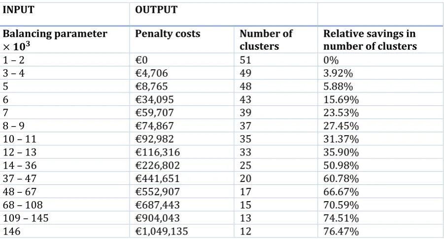
4 When accepting more penalty costs, the number of clusters can be reduced more. A decrease in the number of clusters from 51 to 25 can for example be reached when ASM accepts in total

€226,802 in penalty costs over the 60-year horizon. A decrease from 51 of 12 can be reached when Schiphol accepts €1,049,135 in penalty costs. An important conclusion is that the model

chooses to align the replacements of assets as soon as possible by shifting the assets’ first

replacements, such that the subsequent replacements in the horizon are naturally in cadence and do not need to be shifted anymore. This way, a huge decrease in the number of clusters can be achieved by making relatively small shifts in replacement moments. This is important since it shows us that the impact on operations can be decreased without having to accept increased risks because of postponing assets with many years.

A sensitivity analysis was performed to see how the values for the input parameters influence the solution. We concluded that limiting the years with which an asset may be replaced early or late to only one year influences the solution planning and increases the penalty costs with 64.7% (when ASM wants to decrease the number of clusters to 25) and 190.6% (when ASM wants to decrease the number of clusters to 16). This happens because this setting hinders the model from early synchronizing the replacements and more shifts need to be made. This again stresses the importance of early alignment of replacement cycles.

Another important part of the sensitivity analysis challenges the assumption that the costs for late replacement of assets are linear in the number of years with which an asset was postponed. Moreover, in the original case study the costs for one year of late replacement were set to be more expensive than the costs for one year of early replacement. This resulted in many assets being replaced earlier than optimal and only a little number of replacements being postponed. In the sensitivity analysis we proposed an increasing, non-linear cost structure which in our opinion may better represent the actual situation. We now see that more replacements are postponed and relatively little assets are replaced earlier than optimal. The resulting penalty costs are much lower, but we advise ASM to invest in refining the cost functions in order to obtain a more truthful representation of the penalty costs.

(5)

5

Preface

(6)

6

Glossary

ASM The Asset Management division of Royal Schiphol Group.

AAS Amsterdam Airport Schiphol

Asset Every individual unit that has a significant share in the total cost price of a system and is depreciated separately. All elevators are unique assets.

Asset type All unique assets that fulfil the same function. For example: elevators.

Asset group A set of assets that share the same asset type and construction year. For example: elevators built in 2003.

System A set of assets that together deliver a value to the customer and fulfil a specified function, e.g. the passenger transport system, consisting of the asset types elevators, escalators and moving walkways.

(9)

9

1. Introduction

As one of Europe’s main airport operators, Royal Schiphol Group acts in a rapidly growing market with a rising demand for air transport. Aiming to efficiently fulfil this demand, the company faces complex decisions. In this chapter, we will introduce the problem on which this research will focus. Section 1.1 will provide more information about Royal Schiphol Group. In Section 1.2 we will elaborate on the problem context. In Section 1.3 the goal of this research, together with the associated research questions will be outlined.

1.1. Royal Schiphol Group

Royal Schiphol Group (“Schiphol”) is an operator of airports and is the owner of Amsterdam Airport Schiphol (“AAS”), Rotterdam The Hague Airport and Lelystad Airport. It also has a majority share in Eindhoven Airport. Moreover, the company closely works together with foreign airports. The exploitation of AAS is the company’s main activity. This thesis will focus on AAS only.

The activities at AAS can be subdivided into three business areas, i.e. Aviation, Consumer Products & Services and Real Estate. The key business area is Aviation, which provides service to passengers, airlines, freight handlers and logistics companies. Aviation develops and manages infrastructure that allow for an efficient and reliable movement of passengers, luggage and goods.

The Asset Management division (“ASM”) is responsible for the planning, development, realization,

management and maintenance of the approximately 45,000 assets at AAS. Examples of these assets can be the runways, passenger bridges, aircraft stands, but also climate systems, elevators or lighting.

The ASM division is divided into five subdivisions. The Strategy Office is responsible for aligning the ASM strategy for Aviation with the overall Schiphol strategy. Planning & Portfolio Management

is responsible for translating the customer’s demands into asset planning and Development is

responsible for the actual realization of the asset. After realization the assets are transferred to Maintenance & Operations, which is the division that is responsible for the execution of maintenance on the asset during its life cycle. The fifth subdivision is the Technical Expert Center

(“TEC”).

TEC can be seen as the knowledge center of ASM. TEC draws, manages and improves asset policies and maintenance concepts, taking into account availability and costs, but also aspects such as legislation, sustainability and safety. TEC provides advise in order to optimize asset efficiency, steering at lowering costs, while ensuring that asset performance meets the standards as has been agreed upon internally and with customers. TEC can be further subdivided into four divisions, one

of which is Technical Management (“TM”), the division in which this research will be carried out.

1.2. Problem statement

One of the main tasks of TM is the development of the so-called meerjarenonderhoudsplan

(multi-year maintenance plan, “MJOP”). The main goal of the MJOP is to plan and budget major

maintenance tasks, i.e. renovations and replacements, for the coming five years. The MJOP is updated every year based upon actual asset conditions and performances, resulting in a plan with a rolling horizon. In developing this MJOP, TM closely works together with Maintenance &

(10)

10 Under the current planning approach, decisions are made on asset level – or sometimes even on component level. This approach ensures that the assets are optimally utilized, but the extensive asset base also makes this approach time-intensive and complex. It also results in a high dispersion of activities over time and in many small projects being performed simultaneously. Since these projects have their own project teams, ASM also thinks that overheads costs can significantly be reduced when activities are more clustered. Activities in the MJOP, i.e. in the coming five years, are already clustered as much as possible in order to achieve economies of scale and lower the impact on operations. ASM however believes that planning over a longer time horizon increases predictability and therefore allows for easier integration in daily operations while limiting the disturbance for processes and passengers. The vast number of assets however makes it very hard to determine what optimal packages of maintenance tasks and replacements and when to carry out these clusters.

In addition, ASM believes that the new approach will increase the (timely) realization of maintenance plans. Plans are now often postponed, since maintenance and replacements almost always interfere with the daily operational processes at the airport and may therefore decrease

the passenger’s comfort. ASM thinks that planning longer in advance makes it easier to integrate maintenance in the daily process, since there is more time to come up with additional measures to limit the inconvenience for the passenger. Another reason for the postponements is that maintenance turns out to be hard to sell to customers. It is often not clear to airlines what the added value of maintenance is. This often results in maintenance projects being postponed in order to free budget for new developments.

The fact that ASM is currently on the verge of an organizational change is important for understanding the context of these problems. Schiphol’s strategy is to operate in accordance to a

control model. This allows Schiphol to focus on its core processes and to make optimal use of the expertise of its business partners and suppliers. In the current situation, the actual execution of maintenance is already outsourced to the main contractors. ASM is however still highly involved in developing maintenance concepts, evaluating the need for maintenance and replacements and scheduling on operational level. In the new methodology, the main contractor will have a higher responsibility and act more autonomous. ASM will provide the main contractors with a long-term planning which defines the moments at which major maintenance, overhauls and replacements of assets are planned. This way, ASM is going to make a shift from result-based to performance-based contracts. The responsibility of the main contractor would be to ensure that the asset, or a process as a whole, meets the predefined performance levels until these moments of intervention, by performing regular maintenance. Also the management of asset data, and making predictions on asset performance, degradation and failure behavior on asset level will become the responsibility of the main contractor. In addition, till now contractors were responsible for one technical discipline, for example the buildings itself, building-specific installations and energy production, fire safety or operating assets. From 2019 on, the contractors will be responsible for a geographical area with all technical disciplines within it. The coordination between the different technical disciplines and individual assets therefore becomes more important.

(11)

11

1.3. Research goal

ASM decided that for now the focus should be on the long-term planning of asset replacements. Because of time constraints, the focus of this research will be on the E-pier. This way, a proof of concept will be delivered, which can later on be extended to other areas at AAS. The lifetime for the construction of a pier is 60 years, which is why a planning horizon of 60 years is taken. Many different stakeholders are involved in replacement activities in the terminal. The focus of this research will however be on developing a planning that is optimal from an ASM viewpoint. Therefore, the main research question will be as follows:

How can the Asset Management division of Royal Schiphol Group plan the replacements of assets over a 60 year horizon, in order to limit the impact on operations?

The research question will be answered by answering the following sub questions:

1. What is the current situation and how does the current methodology perform? a. What are relevant developments in the aviation industry? How do these

developments influence the context at AAS?

b. What is the current situation? How does this methodology perform? Based on what characteristics are activities clustered at the moment?

c. What does the asset base of the E-pier look like?

In order to gain insight in the current situation, in Chapter 2 we will discuss the relevant developments in the aviation industry and the context at AAS. We will analyze the current situation and its performance to see what problems result from the current methodology and if there is indeed potential for improvement. Furthermore we will zoom in on our case: the E-pier.

2. What is written in existing literature about maintenance optimization? a. What models for maintenance optimization are known?

b. For what situations are these models suitable?

c. What are the strengths and weaknesses of these models? d. What methods are relevant for ASM?

In Chapter 3, existing methodologies for maintenance optimization are reviewed. Based on their characteristics, we will examine which methods can act as a basis for a model that suits ASM.

3. How can ASM optimally plan its replacement activities in the E-pier?

a. How can we determine the deviation from the optimal moment for an individual asset?

b. How can we express the costs that arise from this deviation? c. What constraints should be incorporated in the model?

d. What assumptions and conditions have to be met in order to ensure validity of the model?

(12)

12 4. What are the benefits of the new methodology?

a. How do the different input parameters influence the outcome of the model? b. What savings can the new methodology obtain? How much would ASM have to

invest to achieve these savings?

In Chapter 5 we will analyze the benefits of long-term replacement planning and the clustering of replacement activities. We will research how the various input parameters influence the solution.

5. How should the new methodology be implemented?

a. What practices do we recommend for the use of the new methodology? b. What conclusions can we draw from this research?

c. On what areas should be focused when ASM wants to develop the model further?

(13)

13

2. Situation analysis

This chapter answers the first sub question:‘What is the current situation and how does the current

methodology perform?’. Section 2.1 will briefly discuss recent developments in the aviation

industry and how these influence the context at Schiphol. Section 2.2 will provide insight in the current methodology. Lastly, Section 2.3 will assess the performance of the current methodology for our case, the E-pier, in specific.

2.1. Developments and context

Over time, AAS has become one of the best connected hub airports in Europe. At the moment, the airport has 326 direct destinations. A wide range of factors such as economic recovery, growing world trade, low oil prices and a higher competition between airlines, has led to a rapid growth of the aviation industry over the last years (Royal Schiphol Group, 2017a). 2017 was AAS’s busiest year ever with 68.5 million passengers: a growth of almost 8% with respect to the year before. The number of seats per air transport movement has increased from 165 in 2016 to 168.6 in 2017. Simultaneously, the average passenger load factor has increased from 83.8% in 2016 to 84.7% in 2017 (Royal Schiphol Group, 2017b). This means airlines not only fly with larger aircraft, but that also the number of seats is used more efficiently. Although AAS has almost reached its air transport movement ceiling of 500,000 starts and landings per year, the number of passengers is therefore expected to grow even further.

The consequences of this growth are twofold. First, increasing passenger numbers imply that the load imposed on the assets at the terminal complex increases too. This might result in undercapacity of for example air treatment- or cooling systems and might accelerate the degradation process of these assets. The need for maintenance might therefore increase and assets may have to be replaced earlier than initially estimated.

At the same time, availability and capacity of the terminal becomes increasingly critical in order to be able to house all these passengers and handle the boarding-, transfer and security processes and smooth flow of passengers. This makes it even more difficult to conveniently integrate major maintenance works and replacements in the daily operational processes. For stakeholders like

Schiphol’s Operations department, Security or airlines, the main priority is continuity and a

minimal disturbance of the daily processes. In earlier years, when there was more flexibility in the capacity at AAS, the short-term approach was sufficient since maintenance could be planned more easily alongside daily processes. Nowadays however, predictability of ASM’s plans becomes more and more important, in order for the different stakeholders in the terminal to be able to prepare for maintenance activities that will heavily impact the processes. In addition, ASM’s experience

with major maintenance at airside, i.e. for example at the runways, has shown that many stakeholders prefer longer, but less frequent disturbances over more dispersed, but smaller disturbances. This demands planning over longer horizons.

2.2. Current methodology

In Section 2.2.1 we elaborate on the current situation and we will analyse to what extent major maintenance tasks and replacements are indeed postponed and what the effects of these postponements are. In Section 2.2.2 it is described how and to what extent major maintenance tasks and replacements are currently clustered.

2.2.1. Description of the current situation

(14)

14 are the relatively small maintenance tasks that can be executed without significantly disturbing the operational processes and have a repetitive character. Examples can be the weekly cleaning, a monthly inspection, yearly lubrication or the replacement of small components. Additional corrective actions are then taken in case of malfunctioning or failure of the asset. These activities do not have their own budgets, but are categorized as operational expenses. On the contrary, major maintenance activities like midlife upgrades, overhauls, refurbishments and replacements do have their own budgets. They aim at significantly improving the current state of the asset and are therefore classified as investments. The duration of these projects is relatively long and they are likely to impact daily operations. As indicated, the planning of these major maintenance tasks and replacements is done in the MJOP.

Decisions for heavy maintenance and replacements are condition-based. In the current methodology, assets are monitored individually, resulting in decisions for replacements being made on asset level. Replacement years can be determined by looking at the expected useful life of an asset, which is defined to be the shortest of the expected technical lifetime and the expected economic lifetime of the asset (Royal Schiphol Group, 2017a). The technical lifetime of an asset is the duration that the asset is functional. The economic end-of-life is the moment from which it becomes financially more attractive to replace the asset for a new asset, for example because the asset becomes less reliable and maintenance costs increase or a new asset can fulfil the desired function more efficient. Determining the useful life of an asset is outside the scope of this research and we assume that either the technical- or economic end-of-life – whichever comes first – is indeed the optimal moment for replacement. Since decisions are made on asset level, it would theoretically be optimal to replace assets at the end of their economic end-of-life. In practice, we see that replacement is often postponed.

Most of the activities on the 2019 MJOP did already appear on the 2018 MJOP. Although many of these activities where classified as activities with a high priority, they again appear on the MJOP of 2019, meaning that they have not been executed yet. Relatively little of them will actually start in 2019. There may be additional activities on the 2018 MJOP that were planned for execution, but may in reality not have been executed. The enormous extent of the MJOP however makes it however difficult to follow-up all activities. There is no general database that keeps track of the realization of the MJOP. We do not know to what extent the MJOP plans have been realized and actual percentages of postponed activities may therefore be even higher. What we do know is that around 50% of the budget of the 2018 MJOP was realized. This does however not say much about the number of activities that was actually executed. It might for example be the case that more than 50% of the activities was executed, but that the related costs were much lower than foreseen.

There are multiple valid reasons for postponing MJOP activities, for example to combine them with future renovation projects to save costs. Many activities are however postponed after finalizing the MJOP, since the scarce capacity in the terminal does not leave any room for major maintenance and replacements to take place. Assets are then kept up and running by performing regular maintenance.

For this research, the most actual asset database was used, containing information about all active assets at AAS, i.e. the assets that are currently in use. The database consists of over 45,000 assets. For our research only the assets in plot 5, related to the terminal and piers are relevant. Filtering the data on location, we find that around 22,393 assets are located in these areas.

(15)

[image:15.595.139.457.148.374.2]

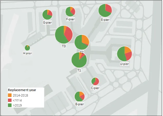
15 plotted in a map of AAS. In red the percentage of assets for which the economic end-of-life was more than five years ago (< 2014), in orange the percentage of assets for which the economic end-of-life was reached somewhere in the last five years (2014 – 2018) and in green the percentage of assets that has not reached its economic end-of-life yet (> 2019). A more detailed view for the E-pier in specific is displayed in Figure 2.

[image:15.595.169.426.407.555.2]

Figure 1. The economic end-of-life of the active assets represented in three categories and visualized in pie-charts over a map of AAS.

Figure 2. The percentage of active assets in the E-pier that has already reached their economic end-of-life is 31%. It can be seen that of these assets, most exceeded the economic end-of-life by 5 years or more.

It is important to realize that it is not necessarily a bad thing when assets are already fully depreciated. A probably better conclusion is that the depreciation period was determined on

conservative estimations of the assets’ economic life spans, which may be perfectly justified for financial reasons. In addition, it is expected that there are gaps between assets’ economic and

(16)

[image:16.595.140.455.174.447.2]

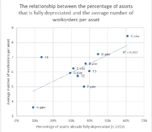
16 between the percentage of assets that was already fully depreciated and the number of work orders. It is important to notice however, that many other factors may influence this relationship. It might for example be the case that assets at Terminal 1 (T1) are used more extensively than assets at the H-pier. Moreover, it can be argued that other measures are more meaningful than the number of workorders, since this measure does for example not take into account the duration of a workorder or the costs related to it. Because of data availability and reliability, we will however not further investigate these relationships.

Figure 3. The average number of workorders in the period 2013-2017 per asset per location plotted against the percentage of assets at that location that have already exceeded their economic end-of-life.

Besides higher maintenance costs, keeping assets in operation much longer than their economic lifetime may have other serious consequences. Assets may be still functioning satisfactory long after their economic end-of-life, but this may come at a risk. Failure of the asset may then result in both high costs and operational disruptions, because spare parts have become obsolete and are not available anymore. Situations like this have not taken place yet and ASM closely monitors the condition of each asset, so this is not probable to happen in the near future either. When the depreciation period however correctly represents the economic lifetime of the asset, it is financially more beneficial to replace the asset for a new model instead of keeping maintaining the old asset. In addition, for many asset types it is likely that a new asset is more efficient than the old asset, for example in terms of output or energy usage.

2.2.2. Clustering in the current methodology

(17)

17 Although the new approach offers more possibilities in clustering, the large size of the asset base and the MJOP makes it hard to manually cluster activities. Before clustering, the MJOP has a size of more than 5,000 rows, where each row corresponds to a maintenance task or replacement. It is not possible, nor desirable, to manually assess all possibilities for clustering. The grouping of activities is at the moment therefore rather pragmatic, instead of a standardized data-based decision-making process in establishing the MJOP.

2.3. Case: the E-pier

For this research, the E-pier at AAS will be taken as a case study. Being built in 1987, the E-pier is one of the oldest piers at AAS. Besides one narrow-body stand, all other 13 stands are suitable for the handling of wide-body airplanes, mainly used by KLM. The E-pier consist of four levels, i.e. the basement, the ground floor, the first floor and the second floor. The basement houses part of AAS’s

luggage handling system, whereas the ground floor houses offices of different airlines. The first- and second floors are the passenger areas. The second floor has been build more recently, i.e. in 2015, as part of the One-XS program in which Schiphol switched from decentralized to centralized security filters.

Taking the E-pier as a case study means that we will focus on gathering data for the assets in this pier and that the model will be tested on the E-pier’s asset base. It is important that we test the

model with a proper representation of the total asset base of the E-pier in order to be able to assess the performance of the current situation and get a good idea of the performance of the model later on. 1,034 were included in the case. An overview of these assets can be found in Appendix A. In Section 2.3.1 we will elaborate on the performance of the current methodology for this dataset.

2.3.1. Performance of the baseline situation

In order to assess the performance of the current methodology over the long term, we have to estimate how we expect the current methodology, which plans over a five-year horizon, behaves over a time period of 60 years. This is difficult since the realization of the plans is currently relatively low. We will therefore differentiate between the current methodology and the ‘baseline situation’ from now on. The baseline situation reflects the situation in which assets are replaced immediately at their end-of-life. Similar to the current methodology, in the baseline situation replacements are planned for all assets separately. In the baseline situation, clustering is therefore merely an indirect result of coinciding replacement moments, but no well-considered decision intending to reduce the impact on operations.

(18)

[image:18.595.71.526.68.261.2]

18 Figure 4. The replacement moments of the assets in the E-pier over the time horizon, resulting in a high number of clusters (51).

ASM believes such a high dispersion of replacements over time comes with many disadvantages. Often mentioned by the different experts that were interviewed is the fact that almost every single replacement is approached as a separate project with its own administrative-, engineering -, and project costs. It is often heard that the lack of clustering results in preparatory activities being executed multiple times. A well-known example is opening up the ceiling in a certain area for the replacement of lighting, closing the ceiling, and opening it again a year later because the sprinklers have to be replaced too. When these replacements were executed together, the needed tools, equipment and labor could have been shared. Maybe even more important is the impact on capacity. During large replacements, parts of the terminal – or in our case the E-pier in specific –

may be inaccessible to passengers, resulting in a disturbed passenger flow or capacity losses. ASM believes that clustering replacements in less but heavier moments, as opposed to many smaller moments highly scattered over time, can decrease the disturbance of the operational processes and result in significant financial benefits. Moreover, ASM thinks the development of a long-term replacement planning has the ability to improve the passenger perception.

Clustering however comes at a cost. We assume that for deviating from the optimal individual replacement moments penalty costs have to be paid. Early replacement of an asset represents a disinvestment, whereas postponed replacement leads to additional maintenance costs. Since in the baseline situation assets are replaced immediately at their economic end-of-life and there are no penalty costs resulting from early replacement or postponement. Therefore, in the baseline

situation the penalty costs are €0. How much penalty costs ASM wants to accept to decrease the number of clusters may differ from location to location, since the preferred outcome of the model may depend on the preferences of internal and external stakeholders at a location. Although a high dispersion is often undesirable, it also results in smaller work packages per cluster and a lower average duration per cluster. In some situations this may be preferred over a low number of clusters. For ASM it is therefore important that the model to be developed can be steered towards more or less clustering in order to be able to roll-out the model to other locations besides the E-pier and take into account the preferences of different stakeholders.

2.4. Conclusion

In this chapter we have answered the research question ‘What is the current situation and how

does the current methodology perform?’. We can answer this question by concluding the following

(19)

19 • Developments in the aviation industry demand a different approach towards the planning of

replacements.

The aviation industry is growing and every year more passengers visit Schiphol. This implies that assets are used more intensively and may increase the need for maintenance. At the same time, capacity becomes more scarce, which demands for ASM to plan over longer time horizons.

• Many assets are already fully depreciated.

This is most likely caused by a conservative estimation of the life spans of the assets, which is not per se a bad thing. When the depreciation period however correctly reflects the economic lifetime of the asset, it may be the case that replacing the old asset for a newer one would financially be the better choice.

• The new methodology offers potential for more clustering.

Since in the new methodology ASM will plan over a longer time horizon and the main contractors will now be responsible for all technical disciplines in a geographical area, there are more possibilities for clustering. The vast size of the asset base makes it however impossible to manually assess all options.

• The baseline situation results in a high dispersion of activities.

o When assets are replaced immediately at their end-of-life, without considering clustering, ASM would have to replace assets in 51 of the 60 years.

o The penalty costs in this situation are €0, since replacements are not shifted.

• What is optimal may differ per location and stakeholder.

(20)

20

3. Literature review

This chapter aims to answer the second sub question: ‘What is written in existing literature about

maintenance optimization?’. We will start this review with brief overview of various maintenance

types in Section 3.1. In Section 3.2 we will focus on common categorizations in various types of maintenance optimization models. Section 3.3 discusses several exact models on the clustering of maintenance activities. Lastly, in Section 3.4 we will the applicability of these models to the situation at Schiphol.

3.1. Preventive maintenance: benefits and disadvantages

Maintenance is defined as those activities that are performed in order to retain systems in, or restore systems to the state that is necessary for fulfilment of its function (Gits, 1992). Corrective maintenance is carried out after a system has failed and therefore reactive in nature. Costs for corrective maintenance are likely to be high, because failure of an asset might result in system downtime, safety dangers, or might cause additional damage to other assets. As opposed to corrective maintenance, preventive maintenance is performed in order to prevent the system from failing and thus has a more proactive character. A special type of preventive maintenance is condition-based maintenance. In condition-based maintenance the execution of maintenance is triggered by inspections or condition measurements (Budai-Balke, 2009). Many argue that this is more effective and efficient than preventive maintenance that is for example solely based on the age of assets. Budai-Balke (2009) however states that predicting failures is often very difficult, which makes it hard to plan maintenance in advance. Budai-Balke (2009) also states that for complex systems it is very hard to monitor all individual units, as well as organize all information in databases. In such complex systems, scheduled maintenance based on ageing might for example be more convenient. Although preventive maintenance aims to minimize the disadvantages of corrective maintenance, it can also result in additional costs since it is likely to result in more maintenance than is strictly needed.

3.2. Categorization of maintenance models

For maintenance models in general, as well for models on clustering in specific, three important categorizations can be recognized. First, the differentiation between single-component and multi-component models, second the differentiation between long and short planning horizons, and third the differentiation between deterministic and stochastic models.

The first differentiation, i.e. between single-component and multi-component models, is most straightforward. A single-component or single-unit model only considers one specific component, whereas multi-component models aim to optimize maintenance policies for a system consisting of several components with or without dependencies between them (Cho & Parlar, 1991).

(21)

21 finite for various reasons. Information is for example often only available for the short term and modifications of the systems may completely change the problem. In finite horizon models, the implicit assumption is made that the system is not used after the horizon. At the end of the horizon the system has totally lost its value or the system is worth its residual value (Dekker et al., 1997). However, assets often have longer lifetimes than the length of the horizon. As a result, many models use a rolling horizon approach (Budai-Balke, 2009; Wildeman et al., 1997). Rolling horizon models aim to capture the advantages of finite- and infinite horizon planning. These models plan over finite horizons, but decisions are based on long-term static planning over the infinite horizon. As Dekker et al. (1997) explain, when planning over rolling horizons, the preliminary long-term planning is adapted to the short-term situation. Decisions for the current finite horizon are implemented and afterwards a new horizon is considered. These models are dynamic in the way that they provide planning rules that can change over the planning horizon, by taking into account non-stationary events. Examples of such non-stationary are varying use and deterioration of assets or unexpected maintenance opportunities that allow for executing maintenance at lower costs.

A final distinction can be made between deterministic and stochastic models. A deterministic model is a model in which, for any value of the decision variables, the corresponding value of the objective function as well as whether or not the constraints will be satisfied is known with certainty (Winston, 2004). In stochastic models, this is uncertain. Likewise, for maintenance in specific, deterministic problems are defined as problems in which the timing and the outcome of maintenance actions are assumed to be certain, whereas in stochastic models this depends on chance (Budai-Balke, 2009). Within stochastic models, Dekker (1996) makes a further distinction between models under risk and models under uncertainty. Here, risk is described as the situation under which the probability distribution of the time to failure is known, whereas in case of uncertainty this distribution is unknown.

3.3. Exact models for maintenance clustering

(22)

22 When reviewing the existing literature, many different approaches to clustering can be found. Let us start with the relatively simple model as proposed in Liang (1985). In this model, the execution moments for individual activities is bounded by time windows. The problem is to find the optimal combination of activities by minimizing the sum of absolute deviations from the execution moments. The approach is pragmatic and helpful when little to no data is available, but it does not include a method to balance the costs of deviating from original execution moments with the savings resulting from the combination of activities. As a result, the model may output multiple different solutions, without being able to determine which one is the best. Moreover, it is assumed that early execution and late execution comes at the same costs and that these costs are equal for all maintenance activities.

Dekker et al. (1992) have extended the heuristic of Liang (1985) by integrating a cost component. In their version of the problem, deviation from the individually planned maintenance activities is not bounded, and one can therefore alter them. The only restriction is that each activity should be performed within the planning horizon. The problem is formulated as a set-partitioning problem, splitting up the set of all activities into subsets where the activities that together form a subset are executed simultaneously. The model aims to find the optimal partitioning, i.e. the partition that minimizes total costs. Since the number of set partitions grows exponentially in the number of maintenance activities complete enumeration of the combinations is impractical. The authors present some theorems that reduce the problem size. The authors acknowledge that in reality penalty functions are often difficult to obtain. In these situations they advise to multiply the absolute deviation from the originally planned execution moment by a scaling factor. If this factor is defined to be low enough, the model will maximize the number of combined activities and simultaneously minimize the sum of the deviations. Dekker et al. (1992) also recognize that identifying the savings resulting from the clustering of activities is in practice very difficult too. Therefore, they assume that all maintenance activities can be divided into groups that share the same preparative work that is unique for that group and that activities in different groups do not share the similar set-up costs. This simplifies the problem since one only has to consider combining activities within one group and that this combination results in the same savings.

In their paper, Wildeman et al. (1997) extend the model in Dekker et al. (1992) and formulated it as a dynamic programming model. They propose a rolling-horizon approach with five phases.

1. Phase 1: decomposition. In this first phase the frequency of the maintenance activity is optimized over an infinite horizon, resulting in maintenance rules for each separate activity. In this phase an average use and deterioration is assumed. Also interactions between components are neglected.

2. Phase 2: penalty functions. For each activity, the additional expected costs of deviating ∆t from the execution time as determined in phase 1 has to be determined. These penalty functions are usually derived from the maintenance models in phase 1.

3. Phase 3: tentative planning. From this phase on, the planning horizon is considered to be finite. Based on the individual maintenance rules of phase 1, together with the current state of the component and additional short-term information, the time ti at which the activity is carried out if it where independent of other activities is determined.

4. Phase 4: grouping maintenance activities. In this phase it is possible to deviate from the tentatively planned execution times for the individual components, in order to make it possible to execute them simultaneously. The optimal grouping structure maximizes the set-up cost reduction minus the costs of deviating from the tentative execution moments, i.e. the penalty costs.

(23)

23 Another clustering model is the Preventive Maintenance Scheduling Problem (PMSP) in Budai-Balke (2009). This is a problem in railway maintenance in which short repetitive activities have to be combined with large projects over a finite horizon and in deterministic time slots. For each routine work, the maximum period between two consecutive executions is given. Moreover, it is known when the activity was executed most recently. It is possible to execute a maintenance activity earlier than necessary, i.e. earlier than the end of its interval. As a result, it is not known beforehand how many executions there will be in the planning horizon. Also a list of projects together with their duration and earliest and latest possible starting times is known. Too early or too late execution of projects is penalized with a cost. Set-up costs are here defined as track possession costs, which are mainly determined by the time that a certain track is unavailable for railway traffic because of maintenance works. The goal is to minimize the sum over the track possession costs and the maintenance costs. The problem is formulated as an linear model. The PMSP can be extended by fixing the intervals between two consecutive executions, i.e. earlier execution is not allowed anymore. This extended version of the PMSP is called the Restrictive Preventive Maintenance Scheduling Problem (RPMSP).

3.4. Applicability to the case

In Section 3.1 we have discussed several types of maintenance. The focus of this research will be on replacements only. As we have seen in Chapter 2, decisions regarding replacements are currently based on the conditions of the individual assets. As suggested by Budai-Balke (2009) this might have several disadvantages. The high complexity and enormous size of the asset base indeed result in a very time-consuming decision making process, losing track of planned and actually executed activities, a high number of postponements and a low level of realization. In line with Budai-Balke (2009), we therefore want to develop a planning in which replacements are planned long in advance.

We saw in literature that when there is dependency between assets, the optimal maintenance schedule for a single asset does not necessarily have to be optimal for the system as a whole as well. This is also the case for ASM. It aims to plan major maintenance on and replacement of assets based on the assets’ individual conditions, since this is assumed to be optimal. However, when zooming out and considering the area – in this case the E-pier – as a whole, we see that this approach results in a high impact on operations caused by the high dispersion of activities. In other words, clustering activities by deviating from these individual execution moments might enable us to find a planning that better fits the preferences of ASM and its customers.

Our approach will follow the framework of Wildeman et al. (1997), where we will focus on phase 4, i.e. the clustering of activities. For this fourth phase we will develop a model based on the work of Budai-Balke (2009). We assume that the frequencies of activities are already optimized in phase 1 of the framework and that this has resulted in optimal replacement years based on the economic end-of-life. We assume an average use and deterioration, which results in the tentative planning in phase 3, which is what we called the baseline situation in Chapter 2. The model is therefore of a deterministic character, i.e. it is assumed that it is known in advance when replacements should be performed. We will also work with a finite horizon. It is therefore assumed that after the horizon the assets will not be used anymore and lose their value. There is no incentive for

executing maintenance just before termination of the horizon in order to end up with ‘healthy’

(24)

24 To tackle the problem in phase 4 of Wildeman et al. (1997) we will develop a model based on Budai-Balke (2009). There are although some significant differences in the problem definition. As we saw, the main goal in Budai-Balke (2009) is to minimize the sum over the maintenance costs, penalty costs and possession costs. In our case we do not directly take into account yearly maintenance costs. We assume that the asset should be replaced anyway, but that the moment of this replacement can be shifted forwards or backwards. In case of an early or late replacement, penalty costs have to be paid. In Wildeman et al. (1997) these costs are determined already in phase 2. In Budai-Balke (2009), penalty costs are charged for the situation in which the last execution is carried out too early compared to the end of the horizon, i.e. the last cycle is too long. We do not take into account such costs, since we assume that the assets should degrade towards the end of the horizon.

Moreover, in Budai-Balke (2009) intervals are restricted (in the RPMSP) or can be executed earlier but not later (in the PMSP). In our case, execution moments can be shifted in both directions, i.e. replacements can be planned both earlier and later than at the end of an asset’s

lifecycle. Moreover, shifts are bounded by a maximum number of years. In addition, our definition of the possession costs differs from that of Budai-Balke (2009). In Budai-Balke (2009) a possession is defined as a railway track that is unavailable due to maintenance works. The costs resulting from a track possession are mainly dependent on the possession time. In our case, a year in which a replacement is planned can be compared to a track possession. During such a

‘possession’, a part of the terminal is unavailable for the operational processes for some time. The financial impact of this unavailability is very hard to determine and depends on several factors, e.g. the exact location of the asset, at what time the replacement is executed and the specific combination of replacements. We will therefore use the number of years in which as least one activity is planned, i.e. the number of clusters, as a measure for possession costs. Our goal is therefore to minimize the penalty costs resulting from early or late execution and the number of clusters in the horizon.

(25)

25

4. Model

In this chapter we want to answer the third sub question: ‘How can ASM optimally plan the replacements of the assets in the E-pier?’. As indicated in Chapter 3, our model is based on Budai-Balke (2009) but is modified in order to fit the situation at ASM. In Chapter 4.1, the description of the model is given. In Chapter 4.2, the mathematical formulation of the model is provided.

4.1. Model description

We want to develop a model that balances the costs and benefits of clustering replacements compared to the individual execution of replacements. Here, the direct cost of clustering is the price that is paid for replacing an asset earlier or later than is optimal for this asset. The benefit of clustering is a lower number of clusters. In order to properly balance the penalty costs and the number of clusters in which replacements are planned, a balancing parameter will be used. This balancing parameter represents the relative weight of penalty costs or the number of clusters. Changing this balancing parameter enables the decision maker to steer the model based on the preferences of users or customers in a certain area of the terminal.

In order for our model to decide in which year to schedule activities, several parameters should be known. First, the year the asset was built or the last replacement year before the start of the planning horizon. Furthermore, we have to know the expected lifetime or economic lifecycle of the asset. Based on the construction year or last replacement of the asset and its lifecycle, we can now determine the first replacement moment of the individual asset in the horizon. Likewise, we can determine the subsequent replacement moments. Shifting these individual moments comes at a certain cost, which can be defined for the individual assets. Moreover, we want to be able to bound the allowed deviation from the optimal replacement moment. In specifying these penalty costs and the maximum allowed deviations we can differentiate between early and postponed replacement.

For now ASM decided not to take into account any workload constraints, i.e. it is assumed that the man-hours available for executing the maintenance works are infinite. This is because the work is outsourced and represents external capacity. In the future, the model can however easily be extended to take into account a maximum workload. Moreover, we assume that all replacements can be executed simultaneously. The scheduling of activities within that year in such a way that contractors can manage the workload is outside the scope of this research.

4.2. Mathematical formulation

Assume that we have a planning horizon of |𝑇| and let 𝑇 be a set of years in which the replacements of an asset 𝑎 need to be scheduled.

Sets

𝐴 set of assets 𝑎

𝑇 years 𝑡 ∈ {1 … 𝑇}

Parameters

𝑃𝐻 planning horizon

𝐵 balancing parameter that balances the importance of clustering as opposed to the penalty costs

(26)

26 𝐴𝐸𝑎 the allowable number of years that the replacement of asset 𝑎 may be executed

early

𝐴𝐿𝑎 the allowable number of years that the replacement of asset 𝑎 may be executed

late

𝑀𝑖𝑛𝑎 𝐿𝐶𝑎− 𝐴𝐸𝑎, the minimum interval between two replacements of asset 𝑎

𝑀𝑎𝑥𝑎 𝐿𝐶𝑎+ 𝐴𝐿𝑎, the maximum interval between two replacements of asset 𝑎

𝐹𝑎 the original first execution moment of the replacement of asset 𝑎 in the time

horizon, without shifting

𝐶𝐸𝑎 the penalty cost for replacing asset 𝑎 one year earlier than at its end-of-life

(linear in the number of years the replacement is planned early)

𝐶𝐿𝑎 the penalty cost for replacing asset 𝑎 one year later than at its end-of-life

(linear in the number of years the replacement is planned late)

Decision variables

𝑥𝑎,𝑡 binary variable that denotes if a replacement of asset 𝑎 is planned in year 𝑡 (1) or

not (0)

𝑦𝑡 binary variable that denotes if at least one replacement is planned in year 𝑡

(𝑦𝑡 = 1 if ∑ 𝑥𝑎 𝑎,𝑡 ≥ 1; 0 if not)

𝐸𝐹𝑎,𝑡 binary variable that denotes if the first replacement of asset 𝑎 is executed early in

year 𝑡

𝐿𝐹𝑎,𝑡 binary variable that denotes if the first replacement of asset 𝑎 is executed late in

year 𝑡

𝐸𝑎,𝑡 binary variable that denotes if a replacement of asset 𝑎 at time 𝑡 is followed by an

early replacement (1) or not (0)

𝐿𝑎,𝑡 binary variable that denotes if a replacement of asset 𝑎 at time 𝑡 is followed by a

late replacement (1) or not (0)

𝑀𝑖𝑛 (𝐵 ∑ 𝑦𝑡 𝑡

+ ∑ ∑ (𝐸𝐹𝑎,𝑡∗ 𝐶𝐸𝑎∗ (𝐹𝑎− 𝑡)) 𝑡=𝐹_𝑎−1

𝑡 𝑎

+ ∑ ∑ (𝐿𝐹𝑎,𝑡∗ 𝐶𝐿𝑎∗ (𝑡 − 𝐹𝑎)) 𝑡=𝐹𝑎+𝐴𝐿𝑎

𝑡=𝐹𝑎+1

𝑎

+ ∑ ∑(𝐸𝑎,𝑡∗ 𝐶𝐸𝑎+ 𝐿𝑎,𝑡∗ 𝐶𝐿𝑎) 𝑡

𝑎

)

s.t.

∑ 𝑥𝑎,𝑡 ≤ 𝑀𝑦𝑡 𝑎

∀𝑡 (1)

∑ 𝑥𝑎,𝑡 𝐹𝑎+𝐴𝐿𝑎

𝑡=𝐹𝑎−𝐴𝐸𝑎

= 1

∀𝑎 (2)

(27)

27 𝑥𝑎,𝑡≤ 𝑀 ∗ 𝐿𝐹𝑎,𝑡 ∀𝑎, 𝐹𝑎< 𝑡 ≤ 𝐹𝑎+ 𝐴𝐿𝑎 (4)

𝑥𝑎,𝑡+ ⋯ + 𝑥𝑎,𝑡+𝑀𝑖𝑛𝑎−1≤ 1 ∀𝑎, ∀𝑡 (5)

𝑥𝑎,𝑡+ ⋯ + 𝑥𝑎,𝑡+𝑀𝑎𝑥_𝑎−1≥ 1 ∀𝑎, ∀𝑡 (6)

𝑥𝑎,𝑡+ ⋯ + 𝑥𝑎,𝑡+𝐿𝐶𝑎−1≤ 1 + 𝑀 ∗ 𝐸𝑎,𝑡 ∀𝑎, ∀𝑡 (7) 𝑥𝑎,𝑡+ ⋯ + 𝑥𝑎,𝑡+𝐿𝐶_𝑎−1≥ 1 − 𝑀 ∗ 𝐿𝑎,𝑡 ∀𝑎, 𝑡 < 𝑃𝐻 − 𝑀𝑎𝑥𝑎+ 2 (8)

The objective function consists of four parts. As explained, the model aims to find the optimum in the trade-off between the penalty costs made for clustering and the number of clusters in which replacements are planned. The first part minimizes the number of clusters. Constraint 1 is related to this first part of the objective function and ensures that the binary variable 𝑦𝑡, which represents

the number of clusters, takes the value 1 when there is at least one replacement planned in year 𝑡.

The second, third and fourth part of the objective function minimize the costs associated to an early or late replacement of an asset. It can be seen, that these costs are determined in different ways. The reason for this is that the penalty costs associated to the first replacement depend on the deviation from the initial first replacement moment 𝐹𝑎 that is given as input to the model,

whereas the penalty costs for the subsequent replacements depend on the previous replacement moments, which are not known beforehand. Let us explain how the model works by an example.

The first replacement

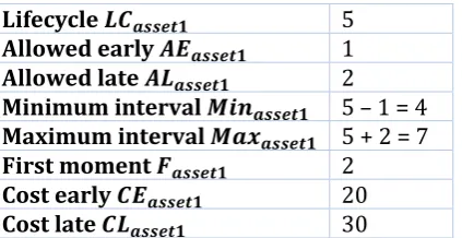
Consider 𝑎𝑠𝑠𝑒𝑡1 with the characteristics as displayed in Table 1.

Lifecycle 𝑳𝑪𝒂𝒔𝒔𝒆𝒕𝟏 5

Allowed early 𝑨𝑬𝒂𝒔𝒔𝒆𝒕𝟏 1

Allowed late 𝑨𝑳𝒂𝒔𝒔𝒆𝒕𝟏 2

Minimum interval 𝑴𝒊𝒏𝒂𝒔𝒔𝒆𝒕𝟏 5 – 1 = 4

Maximum interval 𝑴𝒂𝒙𝒂𝒔𝒔𝒆𝒕𝟏 5 + 2 = 7

First moment 𝑭𝒂𝒔𝒔𝒆𝒕𝟏 2

Cost early 𝑪𝑬𝒂𝒔𝒔𝒆𝒕𝟏 20

Cost late 𝑪𝑳𝒂𝒔𝒔𝒆𝒕𝟏 30

Table 1. Characteristics of the fictional asset 1 in our example.

As mentioned before, the initial first replacement of asset 𝑎 is given by the input parameter 𝐹𝑎.

Constraint 2 ensures that the first replacement of asset 𝑎 is planned somewhere in the allowed interval, based on the value for the initial first replacement of the asset and the allowed early and late execution of the replacement.

The second part of the objective function minimizes the costs associated to an early execution of the first replacement of an asset 𝑎. Since we know beforehand the first initial replacement of an asset, we can check rather easily if this replacement is early or late and what the corresponding penalty costs are.

Assume that solving the model has resulted in the planning as in Table 2. The first replacement has apparently been scheduled in year 𝑡 = 1, meaning that the model should take into account 1 ∗ €20 in penalty costs.

𝒕 1 2 3 4 …

[image:27.595.196.408.373.482.2]

𝒙𝒂𝒔𝒔𝒆𝒕𝟏,𝒕 1 0 0 0 …

Table 2. The first part of the fictional output planning for asset 1 after solving the model.

In constraint 3 it is checked for every 𝑡 < 𝐹𝑎 whether a replacement of asset 𝑎 is scheduled in year

(28)

28 indeed been scheduled in a year 𝑡, the binary early indicator for the first replacement 𝐸𝐹𝑎,𝑡 is

assigned a value 1. If not, 𝐸𝐹𝑎,𝑡 becomes 0. In the second part of the objective function, the penalty

costs for the early first replacements of all assets 𝑎 are determined. For every 𝑡 in the interval [𝑡, 𝐹𝑎− 1] the early indicator for the first replacement 𝐸𝐹𝑎,𝑡 is multiplied by the costs for one year

of early replacement 𝐶𝐸𝑎 and the number of years that the asset was replaced early, i.e. 𝐹𝑎− 𝑡.

Thus, if the value for 𝐸𝐹𝑎,𝑡 is 0, the penalty costs generated for this 𝑡are also € 0.

Looking at Table 3, we can conclude that the correct penalty costs for early replacement have been generated.

Table 3. The functioning of constraint 3 and the second part of the objective function.

Now let us look at the penalty costs for a late first replacement. In constraint 4, for every 𝐹𝑎< 𝑡 ≤

𝐹𝑎+ 𝐴𝐿𝑎 it is checked if a replacement of asset 𝑎 is planned in year 𝑡. If so, the binary late indicator

for the first replacement 𝐿𝐹𝑎,𝑡becomes 1. If not, 𝐿𝐹𝑎,𝑡 becomes 0. Since the first replacement was

planned early and not late, no penalty costs for a late replacement are incurred.

Looking at Table 3 and 4, it can be seen that indeed the right penalty costs are generated for this

first replacement, i.e. €20 for early replacement and €0 for late replacement.

Subsequent replacements

Constraints 5 and 6 plan the subsequent replacements of asset 𝑎. Constraint 5 ensures that in every interval [𝑡, 𝑡 + 𝑀𝑖𝑛𝑎− 1] at most 1 replacement of asset 𝑎 is planned, meaning that it is not

allowed to plan the replacement of an asset 𝑎 at a time 𝑡 earlier than the last replacement plus the minimum interval. Likewise, constraint 6 ensures that in every interval [𝑡, 𝑡 + 𝑀𝑎𝑥𝑎− 1] at least

1 replacement of asset 𝑎 is planned, meaning that it is not allowed to plan the replacement of an asset 𝑎 later than the last replacement plus the maximum interval.

The calculation of the penalty costs of the subsequent replacements is handled in the fourth part of the objective function. Calculating the penalty costs for the subsequent replacements of the asset is somewhat harder than for the first replacement. This is because – for the subsequent replacements – whether the replacement of an asset has been planned early or late depends on when the previous replacement has been planned and we do not know this beforehand.

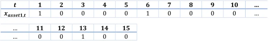
We can solve this problem by counting how many replacements has been planned in certain intervals. Let us again explain this by an example. Assume that solving the model for a planning horizon |𝑇| = 15 results in the planning in Table 5.

𝒕 1 2 3 4 5 6 7 8 9 10 …

𝒙𝒂𝒔𝒔𝒆𝒕𝟏,𝒕 1 0 0 0 0 1 0 0 0 0 …

… 11 12 13 14 15

[image:28.595.168.433.307.348.2]

… 0 0 1 0 0

Table 5. The fictional output planning for asset 1 after solving the model.

As we have seen, the first replacement of the asset asset1 is planned at 𝑡 = 1 and the penalty cost related to this first replacement is already handled by together constraints 3 and 4 and the second part of the objective function.

𝒕 𝑬𝑭𝒂,𝒕 𝑭𝒂− 𝒕 𝑬𝑭𝒂,𝒕∗ 𝑪𝑬𝒂∗ (𝑭𝒂− 𝒕)

1 1 2 – 1 = 1 1 * €20 * 1 = €20

𝒕 𝑳𝑭𝒂,𝒕 𝒕 − 𝑭𝒂 𝑳𝑭𝒂,𝒕∗ 𝑪𝑳𝒂∗ (𝒕 − 𝑭𝒂)

3 0 3 – 2 = 1 0 * €30 * 1 = €0

4 0 4 – 2 = 2 0 * €30 * 2 = €0

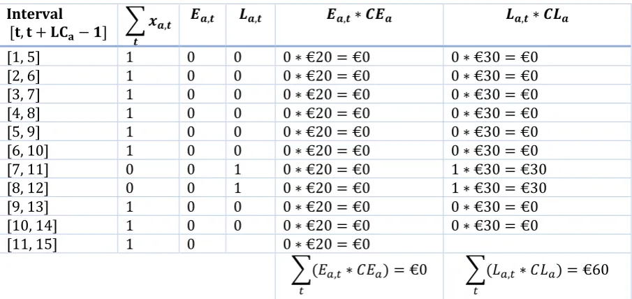
[image:28.595.70.527.638.708.2]

(29)

29 The second replacement is planned exactly at the asset’s end-of-life, i.e. at 𝑡 = 6. The third replacement however planned at 𝑡 = 13 and therefore two years late. The penalty costs for the subsequent replacements of the asset 1 should therefore be 2 𝑦𝑒𝑎𝑟𝑠 𝑙𝑎𝑡𝑒 ∗ 𝐶𝐿𝑎𝑠𝑠𝑒𝑡1.

In the first column of Table 6 the intervals as generated by constraints 7 and 8 are listed. In the second column we calculated the sum of the values for 𝑥𝑎,𝑡 over these intervals. In the third and

fourth column the values that the early-indicator 𝐸𝑎,𝑡 and the late-indicator 𝐿𝑎,𝑡 take for this sum

are shown.

Please note that constraint 8 is only generated for 𝑡 < 𝑃𝐻 − 𝑀𝑎𝑥𝑎+ 2. If constraint 8 is generated

for all values 𝑡 ∈ 𝑇, the late indicator 𝐿𝑎,𝑡 would wrongly become 1 for intervals generated after

the last replacement.

It can be seen that constraint 7 and 8 indeed result in zero years of early replacement and two years of late replacement.

Interval

[𝐭, 𝐭 + 𝐋𝐂𝐚− 𝟏]

∑ 𝒙𝒂,𝒕 𝒕

𝑬𝒂,𝒕 𝑳𝒂,𝒕 𝑬𝒂,𝒕∗ 𝑪𝑬𝒂 𝑳𝒂,𝒕∗ 𝑪𝑳𝒂

[1, 5] 1 0 0 0 ∗ €20 = €0 0 ∗ €30 = €0

[2, 6] 1 0 0 0 ∗ €20 = €0 0 ∗ €30 = €0

[3, 7] 1 0 0 0 ∗ €20 = €0 0 ∗ €30 = €0

[4, 8] 1 0 0 0 ∗ €20 = €0 0 ∗ €30 = €0

[5, 9] 1 0 0 0 ∗ €20 = €0 0 ∗ €30 = €0

[6, 10] 1 0 0 0 ∗ €20 = €0 0 ∗ €30 = €0

[7, 11] 0 0 1 0 ∗ €20 = €0 1 ∗ €30 = €30

[8, 12] 0 0 1 0 ∗ €20 = €0 1 ∗ €30 = €30

[9, 13] 1 0 0 0 ∗ €20 = €0 0 ∗ €30 = €0

[10, 14] 1 0 0 0 ∗ €20 = €0 0 ∗ €30 = €0

[11, 15] 1 0 0 ∗ €20 = €0

∑(𝐸𝑎,𝑡∗ 𝐶𝐸𝑎) 𝑡

= €0 ∑(𝐿𝑎,𝑡∗ 𝐶𝐿𝑎) 𝑡

[image:29.595.72.525.270.484.2]

= €60

Table 6. The intervals as generated by constraints 7 and 8, the values for the sum over the values for xa,t over these intervals, and the resulting values for Ea,t, La,t, Ea,t*CEa and La,t*CLa.

The model has been programmed in AIMMS. Please see Appendix B for the AIMMS syntax.

4.3. Assumptions and conditions to ensure validity of the model

To ensure validity of the model certain conditions need to be met. In constraints 1, 3 and 4 a Big-M parameter is used. This is a parameter with a large number, compared to the associated variables. Since in constraint 1 the values of 𝑥𝑎,𝑡 are summed over the entire time horizon, it is

safe to take a value of Big-M larger than the number of assets. Furthermore, the costs for an early or late replacement should always be ≥ 1 to ensure a correct functioning of constraints 3, 4, 7 and 8. If the costs for early or late replacement are equal to zero, the early and late indicators may arbitrary become 0 or 1. This may result in a replacement being wrongly indicated as being early or late. Moreover, the year for the first replacement should be smaller than the asset’s lifecycle to

ensure a correct functioning of constraints 5 and 6.

For constraint 4 to work correctly, the minimum interval 𝑀𝑖𝑛𝑎 should be larger than the sum of

allowed early and allowed late, i.e. 𝐴𝐸𝑎+ 𝐴𝐿𝑎. If not, the late indicator for the first replacement

𝐿𝐹𝑎,𝑡 can wrongfully be assigned a value 1 when the second replacement of the asset is scheduled

(30)

30 asset, minus the value for allowed early, 𝐿𝐶𝑎− 𝐴𝐸𝑎 should be larger than 𝐴𝐸𝑎+ 𝐴𝐿𝑎. Or: 𝐿𝐶𝑎>

2𝐴𝐸𝑎+ 𝐴𝐿𝑎.

Please note that in this formulation of the model, a replacement just before the end of the horizon is not planned whenever it is not necessary, i.e. when the previous replacement + the maximum interval is outside the planning horizon. In other words, a replacement just before the end of the horizon is only planned when the previous replacement + the maximum interval is inside the horizon. The problem is modelled this way since it is assumed that the pier, and therefore the assets within it, loses its value at the end of the horizon. This means it is beneficial to let the assets degrade towards the end of the horizon as much as possible, since this allows ASM to renovate and upgrade the area as a whole without having to devaluate new and healthy assets. In practice, ASM may choose not to perform a replacement just before the end of the horizon in the knowledge that a major upgrade of the area is planned. This choice may then result in postponing the replacement longer than is usually desired (and longer than is dictated by 𝐴𝐿𝑎), more