Development of an integrated decision support method for municipal infrastructure

Full text

(1)Master thesis Development of an integrated decision support method for municipal infrastructure.. Master thesis Name: Jordy Horstink Date: august, 2017 University of Twente.

(2)

(3) Development of an integrated decision support method for municipal infrastructure. Jordy Horstink. In partial fulfillment of the requirements for the degree of Master of Science in Construction Management and Engineering. University of Twente august, 2017. Under supervision of: Dr. I.Stipanovic prof.dr.ir. A.G. Dorée Mevr. M. Steenberg-Vinke Mevr. J. Walman-Mosterd.

(4) Abstract This research presents a method to determine the optimal maintenance activities and maintenance schedule for interrelated roads and sewers resulting in the lowest life cycle cost (LCC), while preserving the minimal required condition of these assets over a predefined period. A literature study has shown that asset managers are increasingly pressured to reduce costs (Danylo, N. and Lemer, A, 1998). This literature also recognizes the need for integrated decision support systems, but recognizes that the focus has been mainly on optimization within single asset types (Shen, Y., and Spainhour, L., 2001). To develop this method a deterministic LCC model was developed that incorporates interrelated roads and sewers. This model uses condition modelling and condition dependent deterioration models to predict the condition of both assets over a 15 year period. The model uses a genetic algorithm because of its robust searching capabilities and possibility to resolve the complexity of large-size optimization problems in an iterative manner. To show the integration capabilities of the model several maintenance methods and corresponding parameters such as their cost are included in the model, allowing for comparison of long term maintenance schedules. The output of the method is a maintenance schedule that prescribes both the maintenance activities and their schedule to reach the lowest possible LCC. This research shows that integration of different asset types into a single model allows for the optimization of the LCC using a genetic algorithm, which can help to overcome departmental fragmentation issues at municipalities. However, further research is needed to enhance the use of condition modelling and algorithm search capabilities..

(5) Table of Contents Abstract ...................................................................................................................................... 4 1. Introduction ......................................................................................................................... 7. 2. Research objective .............................................................................................................. 9. 3. Points of Departure ........................................................................................................... 10 Asset management ..................................................................................................... 10. 3.2. Asset management methodologies ............................................................................ 13. 3.3. Gap analysis ............................................................................................................... 19. 4. 3.1. Research method ............................................................................................................... 20 Interviews .................................................................................................................. 22. 4.2. Development of method and prototype model .......................................................... 22. 4.3. Evaluation of the model ............................................................................................. 22. 5. 4.1. Multi-Asset Life Cycle Cost Model .................................................................................. 24 Proposed framework .................................................................................................. 24. 5.2. Asset deterioration rates ............................................................................................ 27. 5.3. Optimization for multi-asset relation ......................................................................... 28. 6. 5.1. Application of the LCC model .......................................................................................... 32 6.1. Case study .................................................................................................................. 32. 6.2. Model input................................................................................................................ 33. 6.3. Model process ............................................................................................................ 34. 6.4. Genetic Algorithm ..................................................................................................... 35. 6.5. Output ........................................................................................................................ 38. 7. Sensitivity analysis ............................................................................................................ 39. 8. Discussion ......................................................................................................................... 42. 9. Conclusion ........................................................................................................................ 46. 10. Bibliography .................................................................................................................. 48.

(6) 11. Appendix I Interviews ................................................................................................... 54 11.1 Interview municipality of Zwolle .............................................................................. 54 11.2 Interview municipality of Rijssen-Holten ................................................................. 56 11.3 Interview province of Overijssel ............................................................................... 60. 12. Appendix II Dashboard ................................................................................................. 31.

(7) 1 Introduction Municipalities are increasingly confronted by the deterioration of their infrastructure. Inadequate renewal budgets, climbing renewal deficits, increasing demand levels, and stricter regulation all play a role (Grigg, Neil S., 1999) (Halfawy, M., 2004). The number of insurance claims in the Netherlands due to damaged roads has risen by 60% in the period between 2008 and 2016, according to the Dutch insurer ‘Centraal Beheer’. Municipalities are therefore forced to improve effectiveness of managing their infrastructure assets by adopting more proactive and efficient management strategies. The expertise of many different municipal departments (e.g. roads and wastewater) is needed. It is widely recognized that an integrated approach is needed to resolve these fragmentation issues (Lemer, A.C., 1998; Grigg, Neil S., 2006; Halfawy, M., David Pyzoha, and Taymour ElHosseiny, 2002; Shen, Y., and Spainhour, L., 2001). Danylo and Lemer (1998) describe the main role of an asset management system as an integrator, which can interact with output from many different systems. Although there have been significant research efforts on developing infrastructure management models which support individual management processes, the development of integrated processes for multiple assets has received little attention. In this research a model is developed that can be used to determine the lowest possible life cycle cost for road and sewer assets and helps the asset manager to perform a ‘what if ‘analysis. The model calculates the life cycle costs of interrelated roads and sewer pipes for different maintenance scenarios over a predefined period. Condition modeling is used to predict the need for maintenance or reconstruction, based on the current condition, deterioration and minimum service level. For each condition level maintenance activities and their cost are predefined. To. 7.

(8) cope with the large amount of possible maintenance actions at different intervals a genetic algorithm is used to calculate the most cost effective maintenance actions over the lifespan of the road and sewer. To demonstrate the practical and scientific value of the LCC model it is programmed into Microsoft Excel to be used in a case study. The data required for the life cycle costing case study are obtained through practitioner interviews, literature review and expert review. Existing life cycle cost models were analyzed, modified or supplemented to be used in the model. By employing existing models an overlap is created with current literature, allowing for easier future development. To show how the input parameters of the model influence the outcome a sensitivity analysis was performed. Showing the sensitivity of the integrated model allowed for conclusions to be drawn with regards to the parameters with the most impact on the total life cycle cost. As a result of this an asset manager can adjust the parameters to further optimize the life cycle cost. This report has been structured and divided into chapters in the following manner: Chapter 2 describes the research objective. Chapter 3 describes the latest literature related to asset management and life cycle costing. It also differentiates between what is known and what will be described in this report. Chapter 4 addresses the research method that has been used to fill the knowledge gap described in chapter 2. Chapter 5 reports on the framework that is applied to create the model. Chapter 6 addresses the practical application of the model. Chapter 7 describes the sensitivity analysis of the integrated LCC model. Chapter 8 and 9 discuss the results, implications and conclusions of this research.. 8.

(9) 2 Research objective The main objective of this research is to develop an integrated LCC model to support the decision making process for maintenance actions of road and sewers over a predefined lifespan of the assets. This allows municipalities that have sufficient information about the condition and deterioration of their roads and sewers to quickly determine the integrated life cycle cost and maintenance schedule of their roads and sewers. A case study is performed, allowing the model to be tested and evaluated. In order to fulfill the main research objective described above, the following sub-objectives have been identified: •. Development of a method to integrated maintenance actions of roads and sewers. •. Development of a model, which minimizes the life cycle costs required to maintain the infrastructure at a specified level of service. •. Case study using the model with fictive data to verify the integration of the assets in the model. Fulfilling these objectives allows asset managers to perform ‘what if’ analysis’s in the model, accounting for the relation between roads and sewers and the different maintenance actions (preventive maintenance, reconstruct). It will provide asset managers input allowing them to make better choices in their infrastructure maintenance and optimize the life cycle costs. As well as creating awareness among asset managers about the implications revolving around managing interrelated assets.. 9.

(10) 3 Points of Departure To develop an integrated method for decision making in asset life cycle cost it is important to understand the current municipal assets management practices and their strengths and weaknesses. A large number of pavement management systems (PMS) have been developed in the past, ranging from very simple ones to very sophisticated (Rusua, L.; Sitar Taut, D.A.; Jecan, S., 2004). Research on life cycle cost optimization, condition modelling and different maintenance actions within one type of asset is widely available, research that focusses on the integration of multiple types of assets is scarce. Identifying current practices allows a distinction to be made between what is known and the objective of this research, also known as a gap analysis.. 3.1 Asset management Asset management is defined as a framework for optimizing and implementing decisions on construction, operation, inspection, maintenance, renewal and disposal of infrastructure assets in order to deliver safe and economic infrastructure (IAM, 2010). Asset management integrates maintenance and replacement analysis and the economic and system failure analysis (Kerali, H., 2002). Infrastructure asset management deals with assets that support society, such as roads, railways, water mains, sewers or power grids. These are types of infrastructure that can be considered most critical for most municipalities. To develop an integrated method it is important to recognize that assets management involves many different aspects such as budgeting, prioritization and even politics. The institution of asset management (IAM, 2010) shows the different levels of asset management, starting with the optimization of life cycle activities up to the value for money, obtained from the whole 10.

(11) portfolio of systems, networks, information, people, technology, etc. For an asset management system to function properly it needs to combine monitoring, data collection and decision support systems. This should be done for different types of assets and should be accessible to all parties involved in the infrastructure systems. Assets management strategies Recently, interest in asset management strategies has increased. Brint et al. (2009) have identified three reasons that contribute to the increasing interest in asset management strategies and the need for this research as well. The foremost reason is the aging of infrastructure assets that are required to function longer than initially designed for, even though the required levels of service have risen. Second and third are the decreasing budgets because additional responsibilities for the municipality and a decrease in income. Different types of strategies are used to maintain infrastructure assets (OECD, 2001). An important difference in these strategies is that maintenance can be corrective or preventive (Schneider, J; Gaul, A., 2005). Corrective maintenance is used to bring an asset back to its operational standard and used when the cost and consequences of the asset failing are low. Preventive maintenance is used to prevent future maintenance. Preventive maintenance is performed in intervals to prevent failure and costly repairs. The inspection intervals are mostly based on regulations and the experience of the asset manager. The condition-based maintenance method is a strategy that focusses on the current state as shown by inspection (Schneider, J; Gaul, A., 2005). The goal of this strategy is to perform the maintenance at the most convenient time. This strategy is increasingly used to maintain assets when the condition drops below a certain threshold. A disadvantages of this strategy is that start-up costs are high and quantifying data about the condition of an asset can be difficult. 11.

(12) A risk based maintenance strategy not only considers the condition but also considers the consequences of an asset failing and its impact on the entire network (Schneider, J; Gaul, A., 2005). This translates to a higher inspection and maintenance frequency for high risk assets. Asset managers constantly try to find an optimum between corrective and preventive maintenance. Slowing the aging of the infrastructure by taking preventive measures is becoming increasingly popular. In order to adopt a condition or risk based strategy a condition monitoring system has to be in place (Frangool, D.M.; Liu, M., 2005). Decision making By assigning cost and benefits to a certain project a decision maker can compare all maintenance strategies and decide based on the performance targets and available budget. Objectively determining the benefit of a project can be problematic. Within a greater asset management context, many different performance issues must be considered (Cagle R.F., 2003). Two main techniques are used to choose a solution, prioritization and optimization. Prioritization leads to a list of assets which show a high rate of return on the renewal investment in terms of improving the overall network (Marcelo, D.; Mandri-Perrott, C.; House, S.; Schwartz, J.Z., 2016). Individual asset maintenance plans are then optimized to maximize the ROI (Return on investment) by optimizing budget allocation. The ROI of these complex systems consist of elements such as high asset performance, low risk of failure, and low life-cycle costs. (Halfawy, M.R..; Dridi, L.; Baker, S., 2008).. 12.

(13) 3.2 Asset management methodologies In theory several methodologies and methods are described that can be used for asset management. For the purpose of this research life cycle costing is elaborated, the benefit of using (computer) algorithms to calculate life cycle costs and the use of condition modelling to provide input data. Life cycle costing in maintenance To determine a good asset management strategy input is required about various aspects, as described in chapter 3.1. Life cycle costing (LCC) is another one of these aspects and is defined as a method to determine the cost of an object over its entire service life, allowing different scenarios to be optimized and compared on financial grounds (Rahman, S.; Vanier, D.J., 2004). LCC has proven valuable in investment decisions by providing insight in yearly cost. Every investment decision can be optimized using an LCC-analysis. Therefore LCC is not just relevant for new construction projects, but also for investments in maintenance and reconstruction of assets and thus for this research. Several road authorities worldwide have developed life cycle cost models to reduce the maintenance cost for road infrastructure. Where some models are simple, others include complex calculations of socio-economic costs and road deterioration models. Holmvik and Wallin (2007) studied life cycle cost models in the Nordic countries. They concluded that, while many different models have been developed, none of the models can be used as 'standard' without many improvements because they have been developed for specific projects. The cost of maintenance in the future is subject to a discount factor. The discount factor accounts for the assumption that the value of money changes over time. Especially long term 13.

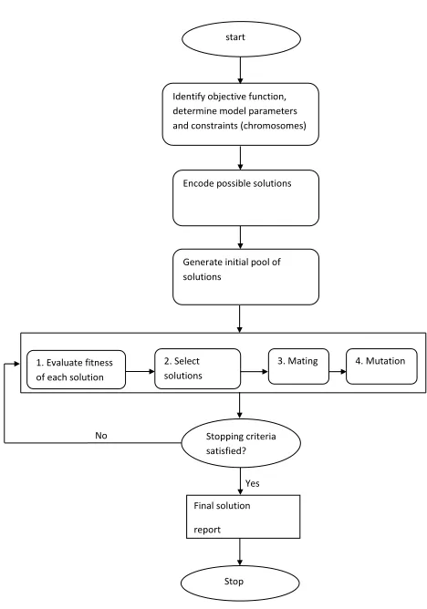
(14) maintenance costs are influenced by the discount rate. Another term for this is net present value, the same amount of money is worth more now than it is in a year (Ross, S., 1995). Algorithms The optimization problem of the integrated LCC model can be described as follows: what are the maintenance actions (maintain, reconstruct) over a predefined lifespan of the road and sewer that results in the lowest life cycle cost. This problem is addressed by adopting a genetic algorithm where the maintenance actions and schedule are planned on a year-by-year basis. Figure 1 shows the steps taken by the algorithm in a flowchart. An algorithm is defined by the Oxford dictionary as: ”A process or set of rules to be followed in calculations or other problem-solving operations, especially by a computer”. Many different types of algorithms exist in theory. For the purpose of this research the focus is Genetic algorithms (GA) because of its suitability to solve large scale, complex problems (Gen, M; Cheng, R., 2000). GA are stochastic search algorithms that uses some basic principles of nature and the evolutionary theory (Gen, M; Cheng, R., 2000). A detailed description of the processes used by genetic algorithms is provided in paragraph 6.4.. 14.

(15) Problem solving using genetic algorithms. start. Identify objective function, determine model parameters and constraints (chromosomes). Encode possible solutions. Generate initial pool of solutions. 1. Evaluate fitness of each solution. No. 3. Mating. 2. Select solutions. 4. Mutation. Stopping criteria satisfied? Yes Final solution report. Stop. Figure 1: Algorithm stages (Morcous, G.; Lounis, G., 2004). 15.

(16) Condition modelling The main objective of this research is to develop an integrated LCC model for roads and sewers systems and perform a case study to verify the integration aspect of the model. The exemplary data used for the case study is derived from road and sewer systems and thus it is relevant to understand the background of condition modelling for these specific types of assets. In order to prioritize the requirements for infrastructure renewal and maintenance there are different condition rating standards available (Kathryn A. Zimmerman, P.E.; Marshall Stivers, P.E., 2007). These standards typically include a point scoring system for each performance indicator (Table 1). Better data availability will typically result in more indicators included in the condition rating system.. Rank 5 4 3. 2 1. Condition rating model Description of Condition Maintenance/renewal Very good condition Only normal maintenance required Minor defects only Maintenance required (5%) Maintenance required to Significant maintenance required (10-20%) return to accepted levels of service Requires renewal Significant renewal/upgrade required (20-40%) Asset unserviceable Over 50% of asset requires replacement. Table 1: condition rating model (International Infrastructure Management Manual, 2015). The starting condition, the deterioration models, the maintenance methods and their cost are integrated into a single model (figure 2).This model has been programmed in Microsoft Excel for convenience and familiarity. For the condition model to function properly the minimum service level and the starting condition need to be entered. The minimum service level is defined by the asset manager and the municipal policy. Certain assets and locations might be prioritized over others. The starting. 16.

(17) condition can based on the last inspection of that asset. An assumption can be made about the starting conditions based on age when there is no inspection data available.. Figure 2: Pavement Condition Index (Shahin, Mohamed Y.; Darter, Michael I.; Kohn, Starr D., 1978). Road condition rating Roads are susceptible to high loads. Large trucks and lorries cause rapid deterioration. Several methods have been developed to predict maintenance costs and remaining service life of different types of roads (Oliveira dos Santos, J.M., 2015). Road deterioration is often modeled as a Markov process resulting in a realistic condition decline on which maintenance decisions can be based. The condition deterioration from this model can then be used to conduct a lifecycle cost analysis (LCCA) by which the total costs over the entire service life of the road can be determined (Smilowitz, K., and Madanat, S., 2000). Following studies have focused on more accurate Markov models such as the continuous-time Markov process (Sathaye and Madanat, 2011) and the semi-Markov model (Zhang and Gao, 2010). The road conditions refers to all kinds of aspects regarding the quality and usability of the roads, for example the road alignment, number of lanes and road roughness. The roughness of the road 17.

(18) is critical in assessing the condition of the road. A deterioration curve can be calculated and calibrated based on past performance and performance of similar roads. The international roughness index (IRI) is an internationally recognized method to determine pavement condition.. Sewer condition rating Wastewater systems are designed to deal with future load condition and are designed to last around 50 years, even though they might be used for much longer. Sewage systems built in during the 60s and 70s are reaching the end of their lifespan, requiring these sewers to be rehabilitated or replaced (Maurer, M., 2009). Proper management of wastewater systems is essential to prevent health hazards (Rutsch et al., 2008) and prevent hydraulic and static deficiencies (Djordjevic et al., 2005). Several deterioration models have been proposed in the literature to predict the deterioration process of individual or grouped pipes. The trouble with predicting condition states of wastewater systems is that there is a lack of complete and reliable data sets. According to (Dirksen, J., Goldina, A., ten Veldhuiz, J.A.E. and Clemens,, 2007) there are also considerable errors in the recording of condition states from camera inspections. The main problem with many deterioration models is the calibration of different parameters. Even when data is available it is not always reliable. Usually data on the condition only contains a snaphot or sample from a single occasion and often contain considerable errors (Ana &Bauwens, 2010). Other wastewater systems are only inspected based on risk assessment providing even fewer data samples.. 18.

(19) Using probabilistic variables requires consideration for different explanatory variables. There are many different processes that can lead to the deterioration and degradation of wastewater systems. Different types of pipes, site conditions, soil conditions, sewage composition and water table conditions impact the deterioration rate (Ana & Bauwens, 2010) .. 3.3 Gap analysis Chapter 3.1 has shown that asset management involves many aspects, levels and strategies. Chapter 3.2 describes different methodologies used in asset management. This paragraph specifies the gap between the literature described in these two paragraphs and the end objective of this research. Current infrastructure maintenance research optimization algorithms focus on the optimization of a single asset type. While these models offer asset managers a great deal of information, they lack integration between different types of assets. Using different models for each asset type results in maintenance schedules that are incompatible, leading to inefficient spending. For example reconstructing a road while the sewer requires maintenance as well, causing damage to the road later on. It is currently unknown how maintenance timing affects the maintenance schedule of other assets, nor is the influence of the minimum service level on the maintenance schedule known. This research aims to find an method that provides an optimal maintenance schedule for the interrelated asset types road and sewers. The integration of condition models provides better insights in how infrastructure assets maintenance schedules are interconnected and how this changes maintenance actions and timing.. 19.

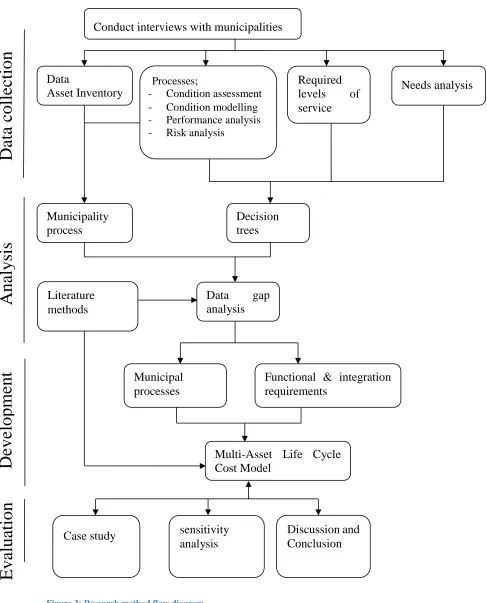
(20) 4 Research method The focus of this research will be on infrastructure management stages to determine the remaining life cycle costs of the different assets, with the possibility to include selection of renewal technologies and costs. The research will consist of four main stages, also shown in figure 3: I.. Interviewing municipalities to review current (asset) management practices;. II.. Analyze municipal infrastructure management processes and compare them to methods described in the literature;. III.. Develop a method and construct a prototype model;. IV.. Perform a case study using the created model;. V.. Analyze results.. 20.

(21) Data Asset Inventory. Evaluation. Required levels of service. Processes; - Condition assessment - Condition modelling - Performance analysis - Risk analysis. Municipality process diagram. Needs analysis. Decision trees. Data gap analysis. Literature methods. Development. Analysis. Data collection. Conduct interviews with municipalities. Municipal processes. Functional & integration requirements. Multi-Asset Life Cycle Cost Model. Case study. sensitivity analysis. Discussion and Conclusion. Figure 3: Research method flow diagram. 21.

(22) 4.1 Interviews The goal of the interviews is to obtain insight on the current methods of municipalities when it comes to the maintenance of infrastructure assets. Appendix I shows the structures and information flow in a municipal infrastructure management process. Every municipality may use different stages or steps as described in the appendix. Three municipalities were interviewed in this research to get a clear image of the management processes and their needs for a decision support method. Identifying the needs of municipalities can help to improve acceptance and the adoption rate of the method. The interviews were held with staff from the departments of sewer and road maintenance.. 4.2 Development of the prototype model Based on the literature study and outcome of the interviews the method is developed. Process modules will be developed in Microsoft excel for testing and evaluation later in the research. The processes that will be included in the method will be discussed further in chapter 5 and chapter 6.. 4.3 Evaluation of the model The multi-asset life cycle cost model will be verified by performing an case study using exemplary data that is based on practical experiences of experts. The developed model was also subjected to a sensitivity analysis to identify the parameters that have the largest influence on the life cycle cost. Example maintenance methods were included to get a realistic image of the remaining life cycle costs. These steps are further explained below.. 22.

(23) Case study Performing a case study verifies that the model is applicable in real world situations. The data used to perform the case study is based on a theoretical situation, in which integration of the two asset types is preferred due to the poor condition of the assets. This approach allows for the results to be analyzed for optimal integration to prove the model functions as intended. Different maintenance actions have a different influence on the condition and remaining life cycle costs of the assets. Predefined maintenance actions and their cost are included in the model to determine the total costs during the remaining life cycle of the assets. Data regarding prices are obtained from municipality databases and construction companies, performance and deterioration models are derived from the NEN guidelines. Sensitivity analysis Analyzing how the uncertainty of the output of the model can be apportioned to the uncertainty in its input can identify factors that have a great influence on the outcome. Factors that have little influence on the outcome can also be identified. A sensitivity analysis will also prove the robustness of the method in the presence of uncertainty.. 23.

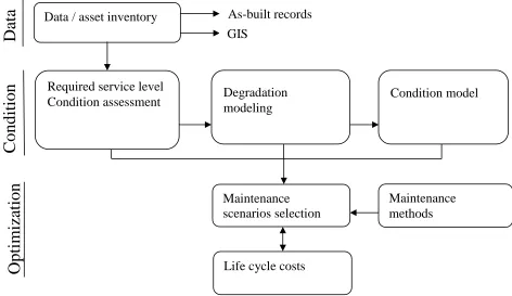
(24) 5 Multi-Asset Life Cycle Cost Model 5.1 Proposed framework The following chapter addresses the three stages identified in the framework used to create the method and as shown in figure 4: First the data requirements of the model are described. Second, the condition models used to predict the future condition of an asset. The last paragraph. Data. Data / asset inventory. Condition. describes the optimization algorithm and the maintenance methods used.. Required service level Condition assessment. As-built records. Multi-Asset Optimization. GIS. Degradation modeling. Condition model. Maintenance scenarios selection. Maintenance methods. Life cycle costs. Figure 4: Conceptual framework. 24.

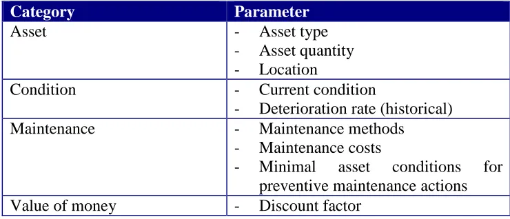
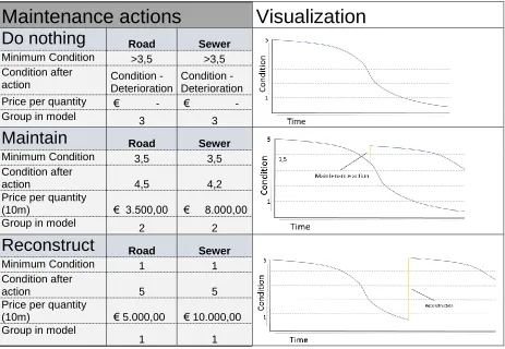
(25) The model requires several types of data to function properly, these data requirements are shown in the table 2. Category Asset. Condition Maintenance. Value of money. Parameter - Asset type - Asset quantity - Location - Current condition - Deterioration rate (historical) - Maintenance methods - Maintenance costs - Minimal asset conditions for preventive maintenance actions - Discount factor. Table 2: data requirements. Firstly a municipality needs to know what assets they have, in what quantity they have them and where they are located. Secondly they need to know the state in which the assets are in, both currently and in the past. Assets that deteriorate quicker will most likely require more maintenance in the future. The maintenance methods for both roads and sewers chosen for this research are displayed in table 3, each represent a single road or sewer section. These methods and their prices have been derived from the CROW website ‘beheerkosten openbare ruimte’ (CROW, 2004).. 25.

(26) Maintenance actions Do nothing Minimum Condition Condition after action Price per quantity Group in model. Maintain Minimum Condition Condition after action Price per quantity (10m) Group in model. Reconstruct Minimum Condition Condition after action Price per quantity (10m) Group in model. Visualization. Road >3,5. Sewer >3,5. Condition Condition Deterioration Deterioration € € 3. 3. Road 3,5. Sewer 3,5. 4,5. 4,2. € 3.500,00. €. 8.000,00. 2. 2. Road 1. Sewer 1. 5. 5. € 5.000,00. € 10.000,00. 1. 1. Table 3: maintenance parameters. Preventive maintenance can be performed as long as the minimum service level for this type of maintenance has not been reached, as shown in figure 3. Afterwards more costly maintenance actions are required.. 26.

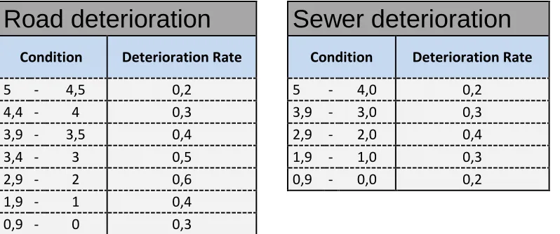
(27) 5.2 Asset deterioration rates Asset deterioration has a negative effect on the overall performance of the structure. Factors that contribute to asset deterioration are time (aging), environmental factors and the asset attributes. Reliable deterioration rates are rarely available for specific assets. Expert judgement data is used in the model for testing purposes. Table 4 shows the deterioration rates that are used in this model for both roads and sewers. figure 5shows these deterioration rates in a graph.. Road deterioration Condition 5 4,4 3,9 3,4 2,9 1,9 0,9. -. Sewer deterioration. Deterioration Rate. 4,5 4 3,5 3 2 1 0. Condition. 0,2 0,3 0,4 0,5 0,6 0,4 0,3. 5 3,9 2,9 1,9 0,9. -. 4,0 3,0 2,0 1,0 0,0. Deterioration Rate 0,2 0,3 0,4 0,3 0,2. Table 4: Road and sewer deterioration rates. Condition. 5 4 3 2. condition road. 1. condition sewer. 0 1. 2. 3. 4. 5. 6. 7. 8. 9. 10 11 12 13 14 15. Time (Years) Figure 5: Visualization of deterioration rates. 27.

(28) 5.3 Optimization for multi-asset relation The suggested method identifies when and which maintenance to perform on either road or sewer on a predefined planning horizon. The decision variables required to perform these actions are identified and explained in this chapter. The proposed formulation uses the following parameters. G= Asset group (road or sewer) T= Number of years in the planning horizon (years) Pgm= Deterioration rate of assets in group g when maintenance m is performed Qg= Quantity of facilities in group g (length or area) Mg= Maintenance costs for maintenance actions (€/unit) Cgt= Condition of group g at the beginning of year t (value 1<x<5) Proposed model The proposed formulation calculates the present value (𝑃𝑉𝑇𝐺 ) of the total cost of maintenance alternatives ,for all assets, implemented over the planning horizon, assuming a discount rate r. 𝐶𝑢𝑟 The objective is to keep the condition of all assets (𝐶𝑔𝑡 ) above a predefined minimum service 𝑇ℎ𝑟 level (𝐶𝑔𝑡 ). Therefore the optimization problem is formulated as follows.. Minimize: 𝑀. 𝑃𝑉𝐺𝑇 = ∑𝑇𝑡=1 ∑𝐺𝑔=1 𝑄𝑔 (1+𝑟𝑔 )𝑡. ∀𝑔, 𝑡. (1). 28.

(29) This formula adds the costs for all asset groups (G), all maintenance actions (Mg), multiplied by their quantity (Qg). Subsequently the cost in time is corrected to the Net Present Value ((1+r)t). Subject to: 𝑇ℎ𝑟 𝐶𝐶𝑢𝑟 𝑔𝑡 ≥ 𝐶𝑔𝑡. ∀𝑔, 𝑡. (2). The current condition of all assets must be greater than or equal to the set threshold. The condition threshold can be changed to suit the needs of the municipality. Where, 1 ≤ 𝐶𝐶𝑢𝑟 𝑔𝑡 ≤ 5 1 ≤ 𝐶𝑇ℎ𝑟 ≤5 𝑔𝑡. (3) (4). The condition of all assets must be between 1 and 5. Condition model Each asset deteriorates at a certain speed depending on the condition. Assets in perfect condition may deteriorate at a different rate than assets in poorer condition. Therefore each condition value has a different yearly deterioration rate. 𝑷𝟓,𝒅 𝒈𝒎 𝟒.𝟗,𝒅 𝑷𝒈𝒎 = ||𝑷𝒈𝒎 || … 𝑷𝟏,𝒅 𝒈𝒎. ∀𝒈, 𝒎. (5). Group g represent the asset group, either road or sewer. Maintenance (m) stands for the current condition of the asset. When no maintenance is performed in a certain year the condition of the asset will fall. When maintenance or a reconstruction is carried out the condition rises to a predefined number. 29.

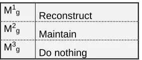
(30) The deterioration rates from the previous years are subtracted from the condition of the previous year to determine the current condition. For example a road with a condition of 4,5 and a deterioration rate of 0,3 will have a condition of 4,5-0,3=4,2 the following year. 𝐶𝑔𝑚𝑡 = ∑𝑮𝒕=𝟏 𝑪𝒈(𝒕−𝟏) − (𝑷𝒈𝒎 ). ∀𝒈, 𝒕. Where, 1 ≤ 𝐶𝑔𝑚𝑡 ≤ 5. (6). (7). Maintenance Three maintenance actions are predefined for each asset in table 5. These include ‘do nothing’, ‘maintain’ and ‘reconstruct’. Costs are determined for each of these maintenance actions for every group (Table 3). M1g M2g M3g. Reconstruct Maintain Do nothing. (8). Table 5: Maintenance groups. Either one of these actions must be performed every year for every asset group. Where 1 ≤ 𝑀𝑔 ≤ 3. (9). The maintenance actions are labeled 1 to 3 for easier processing in the model. Any other value will result in an error.. 30.

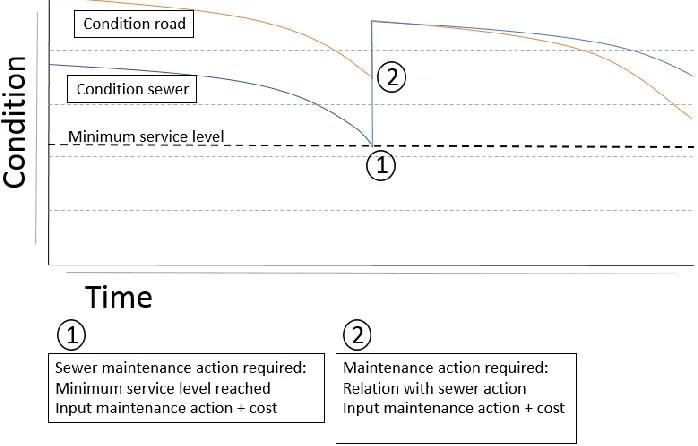
(31) Maintenance actions can only be performed until a certain condition threshold has been passed. When the condition an asset has dropped below the predefined minimum condition level for the preventive maintenance preventive maintenance will no longer be possible. Only the options ‘do nothing’ or reconstruct are available at that time. Integration To guarantee that the maintenance of all assets is coordinated, a link has been made between the assets. When the sewer is being reconstructed the road deteriorates to condition 1 unless the road is being reconstructed as well. This event causes the algorithm to find a maintenance schedule in which the maintenance is combined and optimized. This formula reduces the condition of the road to 1 when the sewer is being reconstructed and the road is not. An example of this is shown in figure 6. 3 𝑀𝑠𝑒𝑤𝑒𝑟 = 𝐶𝑔=𝑟𝑜𝑎𝑑,𝑚=2−3,𝑡 = 1. Figure 6: Example maintenance requirement. 31.

(32) 6 Application of the LCC model This chapter describes the case that was used to test the model and the main components of the model and how they are used.. 6.1 Case study The selected case is a theoretical location somewhere in a typical Dutch municipality, underneath this road lies a sewer system. Both of these assets are approaching their minimum service level and therefore require maintenance. The goal of the municipality is to plan the maintenance so that both road and sewer can be maintained at the same time. This chapter shows how. Figure 7: interrelation between road and sewer. the integration of the assets in the life cycle cost model plans the maintenance activities of the road and sewer and by doing so reduces the amount of money lost due to damaged assets. Sewage pipes are often found under road constructions. Replacing the sewer will damage a large part of the road, as shown in figure 7. Therefore, in the years leading up to the sewage replacement no large maintenance actions should be planned for the road. Preventive maintenance can be performed to postpone bigger maintenance actions.. 32.

(33) 6.2 Model input The condition of the model can be anywhere between 5 and the minimum service level defined by the user. When the minimum service level is reached a maintenance method needs to be applied in that year, resulting in a higher condition and also higher cost. The asset manager also needs to determine the deterioration and minimum service level. The deterioration of an asset can differ greatly due to construction method, usage or the environment. Therefore the deterioration needs to be determined for every asset. Setting a minimum service level allows the model to determine when maintenance is needed. A higher minimum service level will generally result in higher maintenance cost. Lastly the asset manager needs to determine standard maintenance methods. Their cost and conditions can be altered for every municipality, depending on the available options. More maintenance options does require more calculation time. All input parameters can be found in table 6. Category Asset Condition. Maintenance. Value of money. Parameter Asset type Asset quantity Current condition Minimal condition Deterioration rates Maintenance methods Maintenance costs Minimal asset conditions for preventive maintenance actions Discount factor. Road asphalt road 10m2 4 3,5 Table 4 Table 3. Sewer concrete sewer M1 4,5 3,5 Table 4 Table 3. 2%. 2%. Table 6: LCC model input parameters. 33.

(34) 6.3 Model process Whenever the condition of an asset falls behind the minimum service level the model requires a maintenance method to be applied in that year. There are three main reasons why maintenance can be required; •. The minimum service level has been reached:. •. Interrelations with another assets cause a need for maintenance:. •. Preventive maintenance is preferred.. Further, three maintenance alternatives have been identified for every asset. Each maintenance option is linked to a price for that asset type (table 3). Maintaining an asset is usually only possible when the asset is in a certain condition. Once the condition is deteriorated below the threshold for the predefined action the only option is to replace the entire asset. Excel solver fills in the variables, either 1, 2 or 3, corresponding with different maintenance methods. The maintenance methods filled into the model has two effects; it influences the condition of the asset, and it also influences the cost for that year. All maintenance methods combined result in the life cycle cost of that asset (figure 8).. 34.

(35) Figure 8: LCC model stages. 6.4 Genetic Algorithm Chapter 3.2 describes the various stages of genetic algorithms. This chapter describes how those stages match in de model. The excel solver add-in is used as genetic algorithm. The genetic algorithm maintains a ‘population pool’ that describes possible solutions of the given problem. In the LCC model the population consist of all maintenance actions for each year. These actions form the ‘solution’ to the genetic algorithm problem, which is the combined (minimized) life cycle cost for both assets. At the start of the algorithm the population is randomly generated. The solutions of the algorithm are made up of chromosomes. In the model each chromosome represents a single maintenance action for a single asset, either a 1, 2 or 3. Each chromosome consists of genes that can be manipulated by the genetic operator. These genes are represented by a string of symbols which are not visible to the user of the model. The relation between genes, chromosomes and the population can be seen in figure 9.. 35.

(36) Figure 9: Genetic algorithm solution. Each chromosome is associated with a fitness value which is determined by a user defined function, known as the fitness functions. The function returns a value proportional to the solution’s suitability and optimality. Figure 1 shows a simplified flow chart of GA problem solving. At the start of the algorithm the population is randomly generated. The reproduction operator selects chromosomes to be parents for a new chromosome and enters them into the mating pool. Selection of a chromosome can be completely random or based on the fitness of the chromosome. The crossover operator regulates the mating process of two chromosomes. The cross-over rate determines the probability of two parent chromosomes creating a new chromosome. The cross-over rate determines consists of a real number between 1 and 0. The two parent chromosomes are randomly selected from the mating pool. When mating is executed, a new chromosome is created which inherits complementing genetic material from its parents. The Excel solver allows the user to change different settings to optimize the runtime of the algorithm. The settings used during this research are shown in table 7.. 36.

(37) Setting Convergence Mutation rate Population size Random seed Maximum time without improvement Require bounds on variables. Value 0,0001 0,4 0 0 120 No. Table 7: Excel’s Solver settings. The value in the convergence box is the maximum percentage difference in objective values for the top 99% of the population that Solver should allow in order to stop with the message “Solver converged to the current solution.” A smaller value here means that the Solver will take more time, but will stop at a point closer to the optimal solution. The mutation is the relative frequency with which some member of the population will be altered, creating a new trial solution. A higher Mutation Rate increases the diversity of the population and by that the chance that a new, better solution will be found but results in longer processing times. The Population Size is the number of different points (values for the decision variables) that the Evolutionary method to maintains in its population of candidate solutions. The minimum population size is 10. The Random Seed box holds a positive integer number to be used as the fixed seed for a variety of random choices in the Evolutionary method. If this box is left blank the random number generator will use a different seed each time, resulting in different outcomes. The Maximum Time without Improvement is the maximum number of seconds the Evolutionary method continues without improvement in the objective value, before it stops with the message “Solver cannot improve the current solution. 37.

(38) 6.5 Output The output of the model consists of several aspects that are designed to assist the asset manager in the decision making process. Firstly, a maintenance schedule is presented. It shows, both numerical and graphically, when maintenance is performed (Appendix II). This suggests a theoretical optimal time to perform maintenance on both assets. The model also specifies the maintenance method, Showing whether a full reconstruction is needed or a lighter maintenance method will suffice. The cost of these maintenance actions are added for every asset type, resulting in the life cycle cost for that specific asset. These costs can be combined to determine the entire budget needed to maintain the assets over a given period of time. To minimize costs and construction nuisance combining the maintenance of both assets will always be preferred. In the dashboard shown in figure 10 and appendix II it is seen that the algorithm combines the reconstruction of the sewer in year eight with the maintenance of the road. This shows the asset manager that combined maintenance in that time period results in the lowest life cycle cost.. Figure 10: Dashboard condition and cost output example. 38.

(39) 7 Sensitivity analysis A sensitivity analysis is used to show the influence on the outcome of a model by changing different parameters. If the outcome of the model changes more for one parameter than another the model is sensitive to the first variable. The sensitivity analysis is used to show which parameters have the biggest influence on the outcome, the life cycle cost. By changing the deterioration rate, the discount factor and the service level, sensitivities to these variables can be measured. Several parameters have an influence on the outcome of the model. The most important parameters were entered and changed in the model. For every change in an input parameter the algorithm was restarted. After several runs, the cheapest solution was stored and presented in this sensitivity analysis. The results are presented in table 8 and graphed in a spider plot (figure 11).. Parameter. Values. Variable. -20%. -10%. New deterioration rate (road condition 4) LCC Change percentage. 0,36. 0,33. New discount factor LCC Change percentage New service level road/sewer LCC Change percentage. 10%. 20%. 0,27. 0,24. 16100 16357 19062 24028 -16% -14% 0% 26%. 25424 33%. 1,6% 1,8% 2% 2,2% 19607 19332 19062 18797 3% 1% 0% -1%. 2,4% 18537 -3%. 2,8. 3,15. 0% 0,3. 3,5. 3,85. 4,2. 16100 19062 19062 25006 -16% -1% 0% 31%. 35452 86%. Table 8: sensitivity analysis. 39.

(40) Sensitivity spider plot 90%. 70%. 50%. Deterioration Discount factor. 30%. Service level. 10% -20%. -10%. -10% 0%. +10%. +20%. -30% Figure 11: sensitivity spider plot. The results show that the minimum service level has the most influence on the life cycle cost of the assets. An increase of the service level especially requires much additional maintenance. While maintaining a good service level seems beneficial to asset’s service life, it does require much more frequent maintenance. The results also show the number of times maintenance needs to be performed has a big impact on the eventual cost of maintaining the assets. An asset manager might circumvent this by finding cheaper ways of performing preventive maintenance. The current model does not provide these methods. The deterioration rate has a large impact on the life cycle cost as well. The reasoning behind this is similar to the changing service level, substantial additional maintenance is required over the service life of the asset. Figure 5 shows that the deterioration rate has a regressing influence 40.

(41) on the total life cycle cost. This can be explained by the fact that the algorithms picks different maintenance types to decrease the influence of the deterioration rate. The discount factor has a linear influence on the life cycle cost of the assets. However, it does not change the maintenance schedule and therefore has a relatively small influence. However, the rent is always uncertain and therefore remains a risk that needs to be managed. The purpose of mutation is adding diversity to the population. Mutation allows the algorithm to avoid ‘getting stuck’ in a local optimum. To see how the mutation rate influences the life cycle cost they were plotted (figure 12). This showed that only a high mutation rate has a negative impact on the average life cycle cost for a given calculation time.. average PV cost / mutation rate € 28.000,00 € 27.000,00 € 26.000,00 € 25.000,00 € 24.000,00 € 23.000,00. average PV cost. € 22.000,00 € 21.000,00 € 20.000,00 0. 0,1 0,2 0,3 0,4 0,5 0,6 0,7 0,8 Mutation rate. Figure 12 2: mutation rate sensitivity. 41.

(42) 8 Discussion This research has shown a method to integrate different interrelated assets into a single LCC model, which aims to find a maintenance schedule with the lowest life cycle cost for interrelated assets. To find the lowest life cycle cost a genetic algorithm is used which solves the problem ‘what maintenance to perform in what year’. Condition models are programmed for each asset that consider deterioration and the minimum required service level. These condition models were then used to predict the remaining service life of the assets. As a result, the model allows for preventive maintenance to be considered and applied, preventing costly repairs and reconstructions. The model and algorithm This research shows that a large quantity of data is needed to find an optimal maintenance schedule. The starting condition, asset deterioration rate and minimal required service level are the bare minimum of data required to determine the remaining service life of an asset. Additionally, maintenance actions and their impact on all assets are needed to integrate the maintenance schedules of two assets. More importantly, asset managers also have to consider budgets, risks and user delay costs (Danylo, N. and Lemer, A, 1998). Currently combining all this information into the algorithm would make it very complex and prone to error. Future research is needed to identify ways of incorporating additional parameters into the model. The algorithm has been modeled in Microsoft Excel for ease of use, flexibility and its build in evolutionary solver. Microsoft Excel allows for an algorithm to be created without prior computer programming experience. Additionally, Excel also allows easy for visualization and manipulation of the data, which helps with the interpretation of the results. The flexibility 42.

(43) allows for easy alteration of the input parameters, making testing and improving the model possible without great effort. The downside to this evolutionary solver is that it is not very powerful and does not provide insight in its problem solving process. However, the solver does allow many settings of the genetic algorithm to be changed such as the mutation rate and maximum time without a better solution. Viewing the changes these parameters have on the outcome of the model does give some information on the processes used by the algorithm. The LCC model developed uses the input parameters to help the asset manager decide when to perform maintenance and determine the type of maintenance action by providing insight in the preferred maintenance actions, based on asset condition and cost. Furthermore, inefficiencies are removed by integrating the maintenance schedule of the road and the underlying sewer pipes. Reconstructing the sewer, for example, requires digging, thus damaging the road. The main benefit of the presented model as a whole is that it allows asset managers to automatically integrate maintenance schedules of different asset types. In current practices maintenance scheduling requires integration to be performed manually, which is a time-consuming process. Having an overview on when maintenance is performed on every asset allows asset managers to combine maintenance on a network level, improving effectiveness even further. The model also provides the present value life cycle cost for the different asset types. Allowing the available budget to be compared with the required budget. In the event that these budgets don’t match the minimum required service level can be changed to overcome the budget discrepancy. A downside to the use of the developed method is that the deterioration rate and starting condition of both assets are hard to measure objectively. The starting condition can be obtained through inspection or measurements. However, the deterioration rate is harder to obtain because it requires historical data from comparable assets in comparable environments. Obtaining this 43.

(44) information is often a difficult and time consuming process. General deterioration rates can be used, but local deterioration rates may vary greatly. The downside of the model is that it requires the evolutionary solver to solve the large scale problem. The evolutionary algorithm is used to determine a ‘good’ solution and there is no way to be sure that the solution found is the best solution. The case study and ‘hands on’ experience seem to indicate that starting the solver more than once leads to better results than letting it run for a long time. This effect might be caused by the fact that once the solver is stuck in a local optimum, it is unable to find a better global optimum. Restarting the solver allows it to find more than one local optimum. Additionally the evolutionary solver requires substantial calculation time, two minutes per run was used in this research. The required calculation time can be improved by reducing the number of variables the solver needs to change. More specifically, the current algorithm requires the solver to determine a maintenance action for every asset for every year, even though both assets are in perfect condition. To overcome this problem maintenance intervals can be used where the solver only inputs a value where required when an asset falls below the minimum required condition or minimum condition for preventive maintenance. This would reduce the flexibility of the model, but decrease the required calculation time significantly. The method Another shortcoming of the current model is that it doesn’t allow for uncertainty or risk. Many financial decisions are based on their risk profile. Integrating risk into the model can be done by allowing the input parameters to have a standard risk distribution.. 44.

(45) For practical integration of the model in municipal asset management, the model should adopt a standard norm such as the NEN norm for the condition modeling. The model used in this research uses condition models derived from expert judgement. Current literature provides better condition models that provide a more realistic representation of the deterioration of assets. Besides the technical aspects mentioned above, future research should focus more on the needs of asset managers in integration. The factor that has not been validated by the interviews is the need for long term planning among asset managers. The benefits seem clear but none of the interviewed municipalities indicated that they were moving towards long term maintenance scheduling.. 45.

(46) 9 Conclusion The main objective of this research was to develop an integrated method to support the decision making process for integrated infrastructure maintenance. Previous research and tools or models developed only assist decision makers in creating the optimum strategy for single asset types. The combination of different types of infrastructure makes for complex decision making as asset managers at municipalities have to consider many different factors besides the life cycle cost, such as available budget, city planning, innovative construction methods etc. The most important result of this research is that a method is developed that supports the municipality with the integration of interrelated infrastructure assets which leads to more effective decision making. The model that was developed calculates the optimal maintenance strategy according the parameters using deterministic asset deterioration models to predict the remaining service life of the asset. By being able to combine two different asset types, that are interrelated, the model is able to effectively shift maintenance scheduling to allow maintenance actions to be combined. As a result the model shows the year and type of maintenance that should be performed on a project level for both roads and sewers. A municipality can use this information in the decision making process and also change the parameters to perform ‘what if’ analysis. The model uses a genetic algorithm optimization techniques to overcome the computational complexity of the optimization problem. The algorithm was designed to find the lowest life cycle cost over a predefined planning horizon while maintaining a minimum required service level. The case study shows that it is feasible to use genetic algorithms in creating maintenance strategies for different types of infrastructure, while showing the results of this algorithm in a. 46.

(47) structured way to support municipal decision makers. Thereby contributing to current literature that has focused mainly on single asset types. Further research should focus on further improving the model. The sensitivity analysis shows that small changes can have a large impact on the total life cycle cost. This is caused by the fact that the model calculates the life cycle cost on a project level. Altering the model to calculate the costs on a network level results in more predictable and smaller changes to the total life cycle cost, making it more suitable for use in municipal budgeting applications. The reliability of the model can further be improved by incorporating probabilistic calculation methods. This will show uncertainties and risks in the model which can be taken into account when determining the budget for the coming years.. 47.

(48) 10 Bibliography Abaza, K. (2006). Iterative linear approach for Nonlinear Nonhomogenous Stochastic Pavement Management Models. Journal of Transportation Engineering, 244-256. Al-Barqawi, H.; Zayed, T. (2008). Infrastructure Management: Integrated AHP/ANN Model to evaluate municipal water mains' performance. Journal of infrastructure systems, 305318. Ana, E.V. and Bauwens, W. (2010). Modeling the structural deterioration of urban drainage pipes: The state-of-the-art in statistical methods. Urban Water Journal, 47-59. Arayici, Y., Ghassan Aouad, G., Ahmed, V. (2005). Requirements engineering for innovative integrated ICT systems for the construction industry. Construction Innovation Vol. 5, 179-200. Belete Tekie, S. (2014). Integrated Road Asset Management System: The Namibian Experience. IRF Examiner, 12-15. Brint, A., Bridgeman, J., Black, M. (2009). The Rise, Current Position and Future Direction of Asset Management in Utility Industries. Journal of Operational Research Society, 106113. Cagle R.F. (2003). Infrastructure Asset Management: An Eemerging Direction. AACE International transactions, PM21. Camci, F. . (2009). System Maintenance scheduling with PrognosticInformation Using Genetic Algalorithm. IEEE Transactions on reliability, 539-522.. 48.

(49) Christer, A. (1999). Developments in Delay Time Analysis for Modeling Plant Maintenance. Journal of the Operation Research Society, 1120-1137. CROW. (2004, 03 01). Beheerkosten openbare ruimten. Retrieved from CROW: https://www.crow.nl/publicaties/beheerkosten-openbare-ruimte Danylo, N. and Lemer, A. (1998). Asset Management for the Public Works Manager: Challenges and strategies. Dirksen, J., Goldina, A., ten Veldhuiz, J.A.E. and Clemens,. (2007). The role of uncertainty in urban drainage decisions: uncertainty in inspection data and their impact on rehabilitation decisions. Leading Edge Conference on Strategic Asset, 17-19. Djordjevic, S., Prodanovic, D., Maksimovic, C., Ivetic, M. and Savic, D. (2005). Simulation of interaction between pipe flow and surface overland flow in networks. Water Science and technology, 275-283. Frangool, D.M.; Liu, M. (2005). Maintenance and management of civil infrastructure based on condition, safety, optimization, and life-cycle cost∗. Structure and Infrastructure Engineering , 29-41. Ganeshan, R., Grobler, F., Coimbatore, v. (2001). CITYWORK: Application of collaborative technologies for infrastructure management. Computing in Civil Engineering, 74-80. Gen, M; Cheng, R. (2000). Genetic Algorithms & Engineering Optimization. Ashikaga, Japan: John Wiley & Sons, Inc. Grigg, Neil S. (1999). Infrastructure: Integrated Issue or Tower of Babel? Infrastructure systems, 155-117.. 49.

(50) Grigg, Neil S. (2006). Condtion Assessment of water distribution pipes. Infrastructure Systems, 147-153. Gu, N., and London, K. (2010). Understanding and facilitating BIM adoption in the AEC industry. Automation in Construction Vol. 19, 988-999. Halfawy. (2006). Developing enterprise GIS-based data repositories for municipal infrastructure asset management. Joint International Conference on Computing and Decision Making in Civil and Building Engineering. Halfawy, M. (2004). The Interoperability of Geographic Information Systems for Municipal Asset Management Applications. Municipal Infrastructure Investment Planning Project Report. Halfawy, M., David Pyzoha, and Taymour El-Hosseiny. (2002). An Integrated framework for GIS-Based Civil Infrastructure Management Systems. Proc. of the Conference of the Canadian Society for Civil Engineers. Halfawy, M.R..; Dridi, L.; Baker, S. (2008). Integrated decision support system for optimal renewal planning of sewer network. Journal of computing in Civil Engineering, 306372. Hoskins, R., Strbac, G., Brint, A. (1999). Modeling the Degredation of Condition Indices. IEE Proceedings - Generation, Transmission and Distribution, 386-392. IAM. (2010). The Institue of Asset Management. http://www.theiam.org. International Infrastructure Management Manual. (2015). Wellington: The NAMS Groups (NZ).. 50.

(51) Jernigan, F. (2007). BIG BIM little bim. Salisbury: 4site Press. Kathryn A. Zimmerman, P.E.; Marshall Stivers, P.E. (2007). A GUIDE TO MAINTENANCE CONDITION ASSESSMENT SYSTEMS. Urbana: National Cooperative Highway Research Program. Kerali, H. (2002). Road Asset Management. Road Asset Management Principles, 1-13. Kerali, H. (2002). Road Asset Management Principles. Birmingham, UK: The University of Birmingham. L.C. Falls., R. Haas., S. McNeil., S.Tighe. (2001). Asset Management and Pavement Management. Transportation research record, 1-10. Lemer, A.C. (1998). Progress Toward Integrated Infrastructure-Assets-Management Systems: GIS and Beyond. APWA International Public Works Congress. Marcelo, D.; Mandri-Perrott, C.; House, S.; Schwartz, J.Z. (2016). An Alternative Approach to Project Selection: The Infrastructure Prioritization Framework. World Bank PPP Group, 1-40. Maurer, M. (2009). Specific net present value: An improved method for assessing modularisation. Water Research, 2121-2130. Morcous, G.; Lounis, G. (2004). Maintenance optimization of infrastructure networks using. Automation in Construction, 129-142. OECD. (2001). Asset Management For the Roads Sector. Paris: OECD Publications Centre. Oliveira dos Santos, J.M. (2015). A COMPREHENSIVE LIFE CYCLE APPROACH FOR MANAGING. Coimbra: Universtity of Coimbra. 51.

(52) Rahman, S.; Vanier, D.J. (2004). Life cycle cost analysis as decision support tool for managing municipal infrastructure. NRC Publications Record, 1-12. Ross, S. (1995). Uses, Abuses, and Alternatives to the Net-Present-Value Rule. Financial Management, 96-102. Rusua, L.; Sitar Taut, D.A.; Jecan, S. (2004). Integrated Pavement Management System with a Markovian Prediction Model. Journal of Transportation Engineering. Rutsch, M., Rieckermann, J., Cullmann, J., Ellis, J.B., Vollertsen, J. and Krebs, P. (2008). Towards a better understanding of sewer exfiltration. Water Research, 2385-2394. Schneider, J; Gaul, A. (2005). Asset Management Techniques. Power Systems Computing Conference, 1-11. Shahata, K., Zayed, T. (2010). Integrated Decision-Support Framework for Municipal Infrastructure Asset. ASCE Pipeline 2010, 1492-1502. Shahin, Mohamed Y.; Darter, Michael I.; Kohn, Starr D. (1978). Development of a Pavement Condition Index for Roads and Streets. CONSTRUCTION ENGINEERING RESEARCH LAB, 112. Shen, Y., and Spainhour, L. (2001). IT: a potential solution for managing the infrastructure life cycle. Computing in Civil Engineering, 1-2. Smilowitz, K., and Madanat, S. (2000). Optimal Inspection, Maintenance and Rehabilitation Policies for Networks of Infrastructure Facilities Under Measurement and Forecasting Uncertainty. The Journal of Computer Aided Civil and Infrastructure Engineering, 513.. 52.

(53) Vanier, D. J. (2001). Why industry needs asset management tools. Computing in Civil Engineering, 35-43. Zio, E. . (2009). Reliability Engineering: Old Problems and New Challenges. Reliability Engineering and System Safety, 125-141.. 53.

(54) 11 Appendix I Interviews The following stages were used to conduct the interviews 1.. Thematizing: describing the purpose of the interviews. 2.. Designing: Creating the process that lead to fulfilling the purpose of the interview. 3.. Interviewing: Doing the interviews. 4.. Transcribing: Creating a written text of the interview. 5.. Analyzing: Finding the meaning of the information gathered in respect to the research. 6.. Verifying: Verifying the information gathered. 7.. Reporting: Writing the report. 11.1 Interview municipality of Zwolle Data De data wordt bij de gemeente zwollen gekoppeld aan de het GIS systeem. De gegevens over onderhoud en inspecties worden aan de GIS gegevens gekoppeld. Hierdoor is het relatief gemakkelijk om gegevens op te vragen en blijven deze gegevens ook up-to-date. Daarnaast heeft de gemeente Zwolle ook een eigen systeem ontwikkeld waarin al het geplande onderhoud van de komende jaren visueel wordt weergegeven op een kaart. Hierdoor kunnen verschillende afdelingen hun onderhoudswerkzaamheden beter op elkaar afstemmen. Business Processes Bij de gemeente Zwolle wordt gewerkt met beheerpakket Obsurv, welke is ontwikkeld door Grontmij. Dit systeem is geschikt voor verschillende soorten infrastructuur, zoals wegen, 54.

(55) riolering en openbare verlichting. Dit systeem kan aan de hand van inspecties en ouderdom van infrastructuur bepalen welke assets onderhoud behoeven en welke kosten hier globaal aan zijn verbonden. Later wordt bepaald welk onderhoud prioriteit heeft en dus uitgevoerd zal gaan worden. Voor het algemene onderhoud wordt 4 jaar vooruit gepland. Inspecties worden voor algemene middelen elke twee jaar uitgevoerd, hoofdwegen worden elk jaar geïnspecteerd. Wegen worden voornamelijk visueel geïnspecteerd en onderhouden op basis van CROW richtlijnen uit de kwaliteitscatalogus. De inspecties worden uitgevoerd door de leverancier van het beheerpakket. Hierdoor is een partij verantwoordelijk voor het systeem en de gegevens hierin, wat resulteert in een eenvoudiger proces voor de gemeente. Het groenbeheer binnen de gemeente is uitbesteed aam een bedrijf om zo de kosten te drukken. Hierin speelt de gemeente dus alleen nog een regisserende rol. Er is geconstateerd dat er verschil zit in verhardingen op de bedrijventerreinen binnen de gemeente Zwolle. Het bedrijventerrein ‘Hessenpoort’ beschikt over asfaltverharding, terwijl andere bedrijventerreinen een klinkerverharding hebben. Hier zijn meerdere redenen voor genoemd: -. Gebruikerskosten van asfalt zijn lager. Het vervangen van een asfaltlaag is binnen een dag gereed, terwijl het vervangen van een klinkerverharding vaak een week duurt. Goede bereikbaarheid is erg belangrijk voor bedrijven. Om deze reden worden ook geen doodlopende wegen meer gepland op bedrijventerreinen;. -. De uitstraling van het bedrijventerrein ‘Hessenpoort’ werd bij de aanleg als zeer belangrijk ervaren. Omdat her een nieuw bedrijventerrein betrok werd extra aandacht. 55.

(56) besteed aan het zo aantrekkelijk mogelijk maken van het terrein om op deze manier bedrijven aan te trekken en de werkgelegenheid binnen de gemeente te vergroten. Asfalt verhardingen zijn erg kwetsbaar voor achterstallig onderhoud. Wanneer scheuren niet aangepakt worden moet al snel al het asfalt vervangen worden in plaats van alleen de toplaag. Levels of service Het gewenste kwaliteitsniveau is over de hele gemeente gelijk, behalve de binnenstad. De binnenstad krijgt een hogere prioriteit omdat dit als visitekaartje wordt gezien. De zichtbare assets worden getoets aan de kwaliteitscatalogus van de CROW. Er is een toenemende belangstelling voor gebruikerskosten, socialen kwaliteit en overlast. Waar in het verleden de kosten leidend waren, wordt nu steeds meer criteria meegenomen bij het maken van beslissingen. Needs analysis Risico’s worden niet geïdentificeerd, er wordt wel aangegeven dat dit eigenlijk wel zou moeten. Er wordt geen rekening gehouden met bijvoorbeeld incidenten en maar beperkt met gebruikersoverlast tijdens (herstel)werkzaamheden. Langzaam wordt toegewerkt naar een langere termijn planning om te zorgen voor een betere afstemming in de toekomst. Hierbij wordt vooral gekeken naar gemeente Deventer die hier al ver mee zijn.. 11.2 Interview municipality of Rijssen-Holten Data. 56.

(57) In een GIS basiskaart worden alle infrastructurele objecten benoemd. Hierin zijn categorie, functie en invulling benoemd. Riolering en andere ondergrondse infrastructuur zijn hierin niet geïntegreerd. Hiervan zijn tekeningen en ander digitaal kaartmateriaal beschikbaar. In de nabije toekomst zullen deze gegevens wel toegevoegd worden in verband met de wetgeving die dit verplicht. Business processes Periodieke weginspectie elke 2 tot 4 jaar op basis van CROW systematiek. Meet scheuren, vlakheid, rafeling e.d. Op basis van inspectie wordt een waarde toegekend die later door het beheerpakket wordt gebruikt. Vanuit het beheerpakket worden onderhoudsmaatregelen bepaald (maatregelplan). GI NEXT van Oranjewoud. Eenheidsprijzen zitten in de tool van Oranjewoud en CROW. Hierdoor zijn basiskosten inzichtelijk. Er wordt beperkt gekeken naar het verleden om toekomstig onderhoud te voorspellen. Er wordt wel cyclisch gekeken naar het onderhoud. Op basis van aanlegdatum wordt gekeken of een weg vervangen moet worden. Riolering wordt niet in het beheerpakket meegenomen. Een riool in slechte onderhoudsstaat kan nog langer mee dan de weg. Daarom is vaak de weg leidend. Plannen worden van tevoren overlegt met nutsbedrijven om het later opbreken van de straat te voorkomen. Aan de hand van het budget en het beheerpakket wordt de keuze gemaakt welk onderhoud uitgevoerd moet worden en wanneer. Het combineren van verschillend werk gebeurt nu op basis van gevoel. Bijvoorbeeld straatverlichting wordt elke 5 jaar vervangen. Ook asfaltschade wordt vaak gecombineerd om kosten zo laag mogelijk te houden. 57.

(58) Bij het plannen van onderhoud is er geen speciale aandacht voor bedrijventerreinen. De ervaring leert dat dit vaak niet nodig is. Onderhoudsbudget wordt achteraf bijgesteld. Dit wordt genivelleerd over de gehele gemeente. Hierdoor komen grote stijgingen of dalingen weinig voor. Risico’s worden niet geanalyseerd. Wel moet de weg goed genoeg zijn om aansprakelijkheid bij ongelukken te voorkomen. Hierin voorzien de richtlijnen van de CROW. Levels of service Gewenste kwaliteitsniveau niveau B op basis van de CROW voor de hele gemeente. Bedrijventerreinen moeten er goed uitzien om te zorgen dat bedrijven zich graag will vestigen. De gemeente is aansprakelijk wanneer er ongelukken gebeuren. De wegbeheerder kan aantonen dat een weg veilig is d.m.v. inspecties. Onderhoudskosten spelen maar beperkt een rol bij de keuze van nieuw te bouwen infrastructuur. Levenscycluskosten worden dan ook niet in beeld gebracht. Bedrijventerreinen van de jaren 60/70 een facelift gegeven met behulp van subsidie van de provincie. Hoewel de aanwezige infrastructuur nog voldeed is toch de keuze gemaakt om de infrastructuur te vernieuwen. Hierdoor kan uitstraling verbetert worden en mogelijk de werkgelegenheid binnen de gemeente vergroot. Needs analysis Levenscycluskosten worden niet bepaalt, er wordt enkel gerekend over de korte termijn (4 jaar). Door naar de langere termijn te kijken kunnen kosten beter voorspelt worden en kan het. 58.

(59) onderhoud mogelijk beter en efficienter gepland worden. Dit langetermijndenken kan ook een rol spelen bij de aanleg van nieuwe infrastructuur. Ook integratie tussen verschillende soorten infrastructuur is nog suboptimaal. Verschillende afdelingen zijn verantwoordelijk voor bijvoorbeeld wegen en riolering. Door de lange levensduur van rioleringen is wegonderhoud veelal leidend.. 59.

(60) 11.3 Interview province of Overijssel Data The province also used GIS systems to keep track of their infrastructure. The GIS library is steadily increasing with new types of assets. However, not all construction projects were recorded carefully in the past. The data can therefore not be considered a 100% reliable. When errors in the data are found they are corrected immediately, so in the near future the GIS records should be fully up-to-date. Business processes Inspectie op verschillende manieren zoals bijvoorbeeld een boring, stroefheid, etc. Deze gegevens worden geanalyseerd en toegevoegd aan het GIS systeem. Deze gegevens worden voor aanbesteding verfijnd door middel van een visuele inspectie van een expert op het gebied van verhardingen, hierdoor kan het benodigde budget nauwkeuriger worden bepaalt en eventueel onnodig onderhoud voorkomen. Ook kunnen eventuele optimalisaties aan het licht komen door bijvoorbeeld een wegvak samen te voegen en te onderhouden. Hiermee wordt hinder in de toekomst voorkomen. De conditie van de weg wordt bepaalt aan de hand van de inspectierapporten en een jaarlijkse visuele inspectie. De conditie van de weg wordt niet gekwantificeerd, wel wordt de conditie gekoppeld aan het GIS systeem om zo veroudering bij te houden. Aan de hand van deze data kan prioritering plaatsvinden. Een weg die langzaam achteruit gaat krijgt een lagere prioriteit dan een weg met steile daling van kwaliteit. Condition aan de hand van inspecties en 5 jaarsplanning. 1 jaar vooruit gekeken met daadwerkelijke budgettering. Hierna vindt verfijning plaats door te kijken of onderhoud 60.

No results found