Strategy iteration algorithms for games and Markov decision processes

(1)

University of Warwick institutional repository: http://go.warwick.ac.uk/wrap

A Thesis Submitted for the Degree of PhD at the University of Warwick

http://go.warwick.ac.uk/wrap/4526

This thesis is made available online and is protected by original copyright.

Please scroll down to view the document itself.

(2)

M A

E

G NS

I T A T MOLEM

U N

IV ER

SITAS WARWICEN

SIS

Strategy Iteration Algorithms for Games and

Markov Decision Processes

by

John Fearnley

Thesis

Submitted to the University of Warwick

in partial fulﬁlment of the requirements

for the degree of

Doctor of Philosophy

Department of Computer Science

(3)

List of Figures

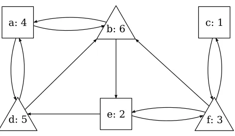
2.1 An example of a parity game. . . 14

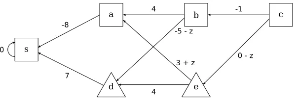
2.2 An example of a mean-payoﬀ game. . . 20

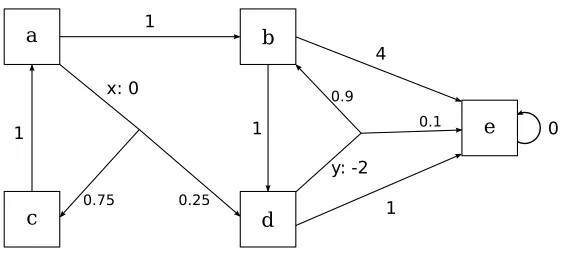
2.3 An example of a Markov decision process. . . 24

2.4 The result of reducing a parity game to a mean-payoﬀ game. . . 36

4.1 A running example for the demonstration of Lemke’s algorithm. . . 71

4.2 The modiﬁed game produced by Lemke’s algorithm. . . 72

4.3 The balance of each vertex in the ﬁrst step of Lemke’s algorithm. . . 73

4.4 The balance of each vertex in the second step of Lemke’s algorithm. 76 4.5 An example upon which the LCP algorithms take exponential time. 97 4.6 The ﬁrst strategy considered in a major iteration. . . 108

5.1 The gadget that will represent the state of a bit. . . 119

5.2 The deceleration lane. . . 121

5.3 The outgoing actions from each bit gadget. . . 121

5.4 The structure that is associated with each bit gadget. . . 123

5.5 The full example with two bit gadgets. . . 125

6.1 A strategy tree. . . 178

(8)

List of Tables

5.1 The deterministic actions in the game_Gn. . . 124

6.1 Experimental results for Friedmann’s examples. . . 199

6.2 Experimental results for the examples of Friedmann, Hansen, and

Zwick. . . 200

(9)

Acknowledgments

First, and foremost, I am indebted to my supervisor, Marcin Jurdzi´nski. His

insis-tence on mathematical rigour and clear thinking have been an inspiration to me,

and the progress that I have made as a researcher can be attributed entirely to him.

I do not think that any of the work in this thesis could have been completed without

his inﬂuence.

I am also indebted to Ranko Lazi´c for acting as my advisor during my studies.

He has never failed to provide sound advice and guidance during my time here. I

would also like to thank Ranko and Kousha Etessami for acting as my examiners,

and for their helpful comments that have greatly improved the ﬁnal version of this

thesis.

I am thankful to the Department of Computer Science at Warwick for hosting

my six year journey from leaving high-school student to the submission of this

thesis. In particular, I would like to thank the members of the DIMAP centre,

the algorithms group, and the formal methods group, for providing a stimulating

environment in which to do research.

Finally, I would like to thank my colleagues and friends: Haris Aziz, Peter

Krusche, Micha l Rutkowski, and Ashutosh Trivedi. My time at Warwick would have

(10)

Declarations

The research presented in Chapter 4 is a joint work with Marcin Jurdzi´nski and

Rahul Savani. My co-authors contributed in the high-level ideas behind the

algo-rithms, but the technical details, along with the lower bounds are my own work. All

other work presented in this thesis has been produced by myself unless explicitly

stated otherwise in the text.

None of the work presented in this thesis has been submitted for a previous

degree, or a degree at another university. All of the work has been conducted

during my period of study at Warwick. Preliminary versions of the work presented

in this thesis have been published, or have been accepted for publication: Chapter 4

has been published in SOFSEM 2010 [FJS10], Chapter 5 has been published in

ICALP 2010 [Fea10b], and Chapter 6 has been accepted for publication at

(11)

Abstract

In this thesis, we consider the problem of solving two player infinite games, such as parity games, mean-payoff games, and discounted games, the problem of solving Markov decision processes. We study a specific type of algorithm for solving these problems that we call strategy iteration algorithms. Strategy improvement algorithms are an example of a type of algorithm that falls under this classification. We also study Lemke’s algorithm and the Cottle-Dantzig algorithm, which are classical pivoting algorithms for solving the linear complementarity problem. The reduction of Jurdziński and Savani from discounted games to LCPs allows these algorithms to be applied to infinite games [JS08]. We show that, when they are applied to games, these algorithms can be viewed as strategy iteration algorithms. We also resolve the question of their running time on these games by providing a family of examples upon which these algorithm take exponential time.

Greedy strategy improvement is a natural variation of strategy improvement, and Friedmann has recently shown an exponential lower bound for this algorithm when it is applied to inﬁnite games [Fri09]. However, these lower bounds do not apply for Markov decision processes. We extend Friedmann’s work in order to prove an exponential lower bound for greedy strategy improvement in the MDP setting.

(12)

Chapter 1

Introduction

In this thesis, we study the problem of solving Markov decision processes and two

player inﬁnite games played on ﬁnite graphs. In particular, we study parity,

mean-payoﬀ, and discounted games. We are interested in strategy iteration algorithms,

which are a speciﬁc type of algorithm that can be used to solve these problems. In

this chapter, we give an overview of the problems that we are considering, and the

results that will be obtained in this thesis. A formal description of these problems

will be given in Chapter 2, and a formal description of the algorithms that we study

will be given in Chapter 3.

1.1 Markov Decision Processes

Markov decision processes were originally formulated in order to solve inventory

management problems. In keeping with this tradition, we will illustrate this model

with a simple inventory management problem. The following example is largely

taken from the exposition of Puterman [Put05].

A manager owns a store that sells exactly one good. At the start of each

month the manager must order stock, which arrives the following day. During

(13)

day of the month. Naturally, the manager cannot know how many orders will arrive

during a given month, but the manager can use prior experience to give a probability

distribution for this. The manager’s problem is to decide how much stock should

be ordered. Since storing goods is expensive, if too much stock is ordered then the

proﬁts on the goods that are sold may be wiped out. On the other hand, if not

enough stock is ordered, then the store may not make as much proﬁt as it could

have done.

This problem can naturally be modelled as a Markov decision process. At

the start of each month the inventory has some state, which is the number of goods

that are currently in stock. The manager then takes an action, by deciding how

many goods should be ordered. The inventory then moves to a new state, which

is decided by a combination of the amount of goods that have been ordered, and

the amount of orders that arrive during the month. Since the number of orders is

modelled by a probability distribution, the state that the inventory will move to in

the next month will be determined by this probability distribution. Each action has

a reward, which is the expected proﬁt from the goods that are sold minus the cost

of storing the current inventory. If this reward is positive, then a proﬁt is made

during that month, and if it is negative, then a loss is made.

A strategy (also known as a policy in the Markov decision process literature)

is a rule that the manager can follow to determine how much stock should be ordered.

This strategy will obviously depend on the current state of the inventory: if the

inventory is almost empty then the manager will want to make a larger order than

if the inventory has plenty of stock.

The problem that must be solved is to ﬁnd an optimal strategy. This is a

strategy that maximizes the amount of proﬁt that the store makes. The optimality

criterion that is used depends on the setting. If the store is only going to be open

for a ﬁxed number of months, then we are looking for an optimal strategy in the

(14)

that is made while the store is open. On the other hand, if the store will remain

open indeﬁnitely, then we are looking for an optimal strategy in the average-reward

criterion. This is a strategy that maximizes the long-term average proﬁt that is

made by the store. For example, the strategy may make a loss for the ﬁrst few

months in order to move the inventory into a state where a better long-term average

proﬁt can be obtained. Finally, there is the discounted-reward criterion, in which

immediate rewards are worth more than future rewards. In our example, this could

be interpreted as the price of the good slowly falling over time. This means that

the profit in the first month will be larger than the profits in subsequent months.

The study of Markov decision processes began in the 1950s. The ﬁrst work on

this subject was by Shapley, who studied two player stochastic games [Sha53], and

Markov decision processes can be seen as a stochastic game with only one player.

The model was then developed in its own right by the works of Bellman [Bel57],

Howard [How60], and others. Puterman’s book provides a comprehensive modern

exposition of the basic results for Markov decision processes [Put05].

Markov decision processes have since been applied in a wide variety of areas.

They have become a standard tool for modelling stochastic processes in operations

research and engineering. They have also found applications in computer science.

For example, they are a fundamental tool used in reinforcement learning, which is

a sub-area of artiﬁcial intelligence research [SB98].

These applications often produce Markov decision processes that have very

large state spaces, and so ﬁnding fast algorithms that solve Markov decision

pro-cesses is an important problem. It has long been known that the problem can be

formulated as a linear program [d’E63, Man60], and therefore it can be solved in

polynomial time [Kha80, Kar84]. However, this gives only a weakly polynomial

time algorithm, which means that its running time is polynomial in the bit length

of the numbers occurring in its inputs. There is no known strongly polynomial time

(15)

1.2 Two Player Games

The deﬁning text on game theory was written by von Neumann and Morgenstern in

1944 [vM44]. Part of this work was the study of two player zero-sum games, which

are games where the goals of the two players are directly opposed. The zero-sum

property means that if one player wins some amount, then the opposing player loses

that amount. A classical example of this would be a poker game, where if one player

wins some amount of money in a round, then his opponents lose that amount of

money. These are the type of game that will be studied in this thesis.

Game theory can be applied to to produce a diﬀerent type of model than

those models that arise from Markov decision processes. In many systems it is

known that there can be more than one outcome after taking some action, but there

may not be a known probability distribution that models this uncertainty about

the environment. Game theory can be used to model this, by assuming that the

decisions taken by the environment are controlled by an adversary whose goal is to

minimize our objective function.

For example, let us return to our inventory control problem. To model this

as a Markov decision process, we required a probability distribution that speciﬁed

the number of orders that will be placed by customers in each month. Now suppose

that we do not have such a probability distribution. Instead, we are looking for

a strategy for inventory control which maximizes the proﬁt no matter how many

orders arrive during each month. To do this, we can assume that the number of

orders that are placed is controlled by an adversary, whose objective is to minimize

the amount of proﬁt that we make. If we can devise a strategy that ensures a certain

amount of proﬁt when playing against the adversary, then this strategy guarantees

that we will make at least this amount of proﬁt when exposed to real customers.

From this, we can see that playing a game against the adversary allows us to devise

(16)

We will study two player inﬁnite games that are played on ﬁnite graphs.

In particular, we will study mean-payoﬀ games and discounted games. These are

similar to Markov decision processes with the average-reward and discounted-reward

optimality criteria, but where the randomness used in the Markov decision process

model is replaced with an opposing player. The objective in these games is again

to compute an optimal strategy, but in this case an optimal strategy is one that

guarantees a certain payoﬀ no matter how the opponent plays against that strategy.

These games have applications in, for example, online scheduling and online string

comparison problems [ZP96].

Whereas the problem of solving a Markov decision process can be solved in

polynomial time, there is no known algorithm that solves mean-payoﬀ or discounted

games in polynomial time. However, it is known that these games lie in the

com-plexity class NP_∩co-NP [KL93]. This implies that the problems are highly unlikely

to be NP-complete or co-NP-complete, since a proof of either of these properties

would imply that NP is equal to co-NP.

In fact, it is known that these three problems lie in a more restricted class

of problems. A common formulation for the complexity class NP is that it contains

decision problems for which, if the answer is yes, then then there is a witness of

this fact that can be veriﬁed in polynomial time. The complexity class UP contains

decision problems for which, if the answer is yes, then there is a unique witness of

this fact that can be veriﬁed in polynomial time. The complexity class co-UP is

deﬁned analogously. Jurdzi´nski has shown that the problem of solving these games

lies in UP∩co-UP [Jur98].

The complexity status of these games is rather unusual, because they are

one of the few natural combinatorial problems that lie in UP ∩ co-UP for which

no polynomial time algorithm is known. This complexity class is also inhabited by

various number theoretic problems such as deciding whether an integer has a factor

(17)

there are few combinatorial problems that share this complexity.

Membership of NP_∩ co-NP does not imply that a problem is hard. There

have been problems in this class for which polynomial time algorithms have been

devised. For example, the problem of primality testing was known to lie in NP_∩

co-NP, and was considered to be a hard problem. Nevertheless, Agrawal, Kayal, and

Saxena discovered a polynomial time algorithm that solves this problem [AKS04].

Another example is linear programming, which was shown to be solvable in

polyno-mial time by Khachiyan [Kha80]. Finding a polynopolyno-mial time algorithm that solves

a mean-payoﬀ game or a discounted game is a major open problem.

1.3 Model Checking And Parity Games

The ﬁeld of formal veriﬁcation studies methods that can be used to check whether a

computer program is correct. The applications of this are obvious, because real world

programs often contain bugs that can cause the system to behave in unpredictable

ways. On the other hand, software is often entrusted with safety critical tasks, such

as ﬂying an aeroplane or controlling a nuclear power plant. The goal of veriﬁcation

is to provide tools that can be used to validate that these systems are correct, and

that they do not contain bugs.

Model checking is one technique that can be used to verify systems [CGP99].

The problem takes two inputs. The ﬁrst is a representation of a computer program,

usually in the form of a Kripke structure. This structure represents the states that

the program can be in, and the transitions between these states that the program

can make. The second input is a formula, which is written in some kind of logic.

The model checking problem is to decide whether the system satisﬁes the formula.

This problem can be rephrased as a problem about a zero-sum game between

two players. This game is played on a graph, which is constructed from the system

(18)

described by the formula, and the other player is trying to prove the opposite.

Therefore, a model checking problem can be solved by deciding which player wins

the corresponding game.

The type of game that is played depends on the logic that is used to

spec-ify the formula. The modal µ-calculus is a logic that subsumes other commonly

used temporal logics, such as LTL and CTL* [Koz82]. When the input formula

is written in this logic, the corresponding model checking game will be a parity

game [EJS93, Sti95]. Therefore, fast algorithms for solving parity games lead to

faster model checkers for the modal µ-calculus. Parity games also have other

ap-plications in, for example, checking non-emptiness of non-deterministic parity tree

automata [GTW02].

Parity games are strongly related to mean-payoﬀ games and discounted

games. There is a polynomial time reduction from parity games to mean-payoﬀ

games, and there is a polynomial time reduction from mean-payoﬀ games to

dis-counted games. Parity games are also known to be contained in UP∩ co-UP, and

no polynomial time algorithm is known that solves parity games. Finding a

poly-nomial time algorithm that solves parity games is a major open problem, and this

also further motivates the study of mean-payoﬀ and discounted games.

1.4 Strategy Improvement

Strategy improvement is a technique that can be applied to solve Markov decision

processes and inﬁnite games. Strategy improvement algorithms have been devised

for all three optimality criteria in MDPs [Put05], and for all of the games that we

have introduced [Pur95, BV07, VJ00]. Strategy improvement algorithms fall under

the umbrella of strategy iteration algorithms, because they solve a game or MDP by

iteratively trying to improve a strategy. We will introduce the ideas behind strategy

(19)

The problem of solving a linear program can naturally be seen as the problem

of ﬁnding a vertex of a convex polytope that maximizes an objective function. The

simplex method, given by Dantzig [WD49, Dan49], takes the following approach to

ﬁnding this vertex. Each vertex of the polytope has a set of neighbours, and since

the polytope is convex, we know that a vertex optimizes the objective function if and

only if it has no neighbour with a higher value. Therefore, every vertex that is not

optimal has at least one neighbour with a higher value. The simplex method begins

by considering an arbitrary vertex of the polytope. In each iteration, it chooses some

neighbouring vertex with a higher value, and moves to that vertex. This process

continues until an optimal vertex is found.

Since there can be multiple neighbours which oﬀer an improvement in the

objective function, the simplex method must use a pivot rule to decide which

neigh-bour should be chosen in each iteration. Dantzig’s original pivot rule was shown to

require exponential time in the worst case by a result of Klee and Minty [KM70]. It is

now known that many other pivot rules have exponential running times in the worst

case, and there is no pivot rule that has a proof of polynomial time termination. On

the other hand, the simplex method has been found to work very well in practice

because it almost always terminates in polynomial time on real world examples. For

this reason, the simplex method is still frequently used to solve practical problems.

Strategy improvement uses similar techniques to those of the simplex

algo-rithm in order to solve MDPs and games. For each strategy, the set of neighbouring

strategies that secure a better value can be computed in polynomial time, and it can

be shown that a strategy is optimal if and only if this set is empty. Therefore,

strat-egy improvement algorithms begin with an arbitrary stratstrat-egy, and in each iteration

the algorithm picks some neighbouring strategy that secures a better value.

Strategy improvement algorithms also need a pivot rule to decide which

neighbouring strategy should be chosen. In the context of strategy improvement

(20)

it has been shown that using an unsophisticated switching policy can cause the

algorithm to take exponential time [MC94]. However, no exponential lower bounds

were known for more sophisticated switching policies. In particular, the greedy

policy is a natural switching policy for strategy improvement, and it was considered

to be a strong candidate for polynomial time termination for quite some time. This

was because, as in the case of linear programming, the greedy switching policy was

found to work very well in practice. However, these hopes were dashed by a recent

result of Friedmann [Fri09], in which he constructed a family of parity games upon

which the strategy improvement algorithm of V¨oge and Jurdzi´nski equipped with

the greedy switching policy takes exponential time. These results have been adapted

to show exponential lower bounds for greedy strategy improvement algorithms for

mean-payoﬀ and discounted games [And09].

1.5 The Linear Complementarity Problem

The linear complementarity problem is a fundamental problem in mathematical

programming [CPS92], which naturally captures the complementary slackness

con-ditions in linear programming and the Karush-Kuhn-Tucker concon-ditions of quadratic

programs. The linear complementarity problem takes a matrix as an input. In

general, the problem of ﬁnding a solution to a linear complementarity problem is

NP-complete [Chu89]. However, when the input matrix is a P-matrix, the problem

is known to belong to the more restrictive class PPAD [Pap94]. This class is known

to have complete problems, such as the problem of ﬁnding a Nash equilibrium in

a bimatrix game [DGP06, CDT09], but it is not known whether the P-matrix

lin-ear complementarity problem is PPAD-complete. On the other hand, there is no

known polynomial time algorithm that solves P-matrix LCPs, and ﬁnding such an

algorithm is a major open problem.

(21)

algo-rithm, because it uses pivotal algebra to move from one vertex of the polytope to

the next. Pivoting algorithms have also been developed to solve the linear

com-plementarity problem. Prominent examples of this are Lemke’s algorithm [Lem65],

and the Cottle-Dantzig algorithm [DC67]. Although these algorithms may fail to

solve an arbitrary LCP, both of these algorithms are guaranteed to terminate with

a solution when they are applied to a P-matrix LCP.

Recently, the inﬁnite games that we are studying have been linked to the

linear complementarity problem. Polynomial time reductions from simple stochastic

games [Con93] to the linear complementarity problem have been proposed [GR05,

SV07]. Simple stochastic games are a type of game that also incorporate random

moves, and it has been shown that the problem of solving a discounted game can

be reduced to the problem of solving a simple stochastic game [ZP96]. Also, a

direct polynomial time reduction from discounted games to the P-matrix linear

complementarity problem has been devised by Jurdzi´nski and Savani [JS08]. These

reductions mean that the classical pivoting algorithm from the LCP literature can

now be applied to solve parity, mean-payoﬀ, and discounted games.

1.6 Contribution

In Chapter 4, we study how the pivoting algorithms for the linear complementarity

problem behave when they are applied to the LCPs that arise from the reduction

of Jurdzi´nski and Savani. We show that Lemke’s algorithm and the Cottle-Dantzig

algorithm can be viewed as strategy iteration algorithms, and we present versions of

these algorithms that work directly on discounted games, rather than on the LCP

reductions of these games. This allows researchers who do not have a background in

mathematical optimization, but who are interested in solving games, to understand

how these algorithms work.

(22)

are applied to P-matrix LCPs [Mur78, Fat79], it was not known whether these

bounds hold for the LCPs that arise from games. It is possible that the class of

LCPs generated by games may form a subclass of P-matrix LCPs that is easier to

solve. We show that this is not the case, by providing a family of parity games upon

which both Lemke’s algorithm and the Cottle-Dantzig algorithm take exponential

time. Since parity games lie at the top of the chain of reductions from games to the

linear complementarity problem, this lower bound also holds for mean-payoﬀ and

discounted games. The work in this chapter is joint work with Marcin Jurdzi´nski

and Rahul Savani, and it is a revised and extended version of a paper that was

published in the proceedings of SOFSEM 2010 [FJS10].

In Chapter 5, we study strategy improvement algorithms for Markov decision

processes. The greedy switching policy was a promising candidate for polynomial

time termination in both game and MDP settings. For parity games, the result of

Friedmann [Fri09] proved that this was not the case. However, while Friedmann’s

examples have been adapted to cover mean-payoﬀ and discounted games, no

expo-nential lower bounds have been found for greedy strategy improvement for Markov

decision processes. We resolve this situation by adapting Friedmann’s examples to

provide a family of Markov decision processes upon which greedy strategy

improve-ment takes an exponential number of steps. This lower bound holds for the

average-reward criterion. The work presented in this chapter is a revised and extended

version of a paper that was published in the proceedings of ICALP 2010 [Fea10a].

In Chapter 6, we study strategy improvement algorithms for parity games

and mean-payoﬀ games. With the recent result of Friedmann, doubts have been cast

about whether strategy improvement equipped with any switching policy could

ter-minate in polynomial time. This view is reinforced by a recent result of Friedmann,

Hansen, and Zwick [FHZ10], who showed that random facet, another prominent

switching policy, is not polynomial.

(23)

im-provement follow simple rules, and do not take into account the structure of the

game that they are solving. In this chapter, we show that switching policies can

use the structure of the game to make better decisions. We show that certain

struc-tures in parity and mean-payoﬀ games are strongly related with the behaviour of

strategy improvement algorithms. Moreover, we show that switching policies can

exploit this link to make better decisions. We propose an augmentation scheme,

which allows traditional switching policies, such as the greedy policy, to take

advan-tage of this knowledge. Finally, we show that these ideas are also exploited by the

recent super-polynomial lower bounds, by showing that the augmented version of

the greedy policy is polynomial on Friedmann’s examples, and that the augmented

version of random facet is polynomial on the examples of Friedmann, Hansen, and

Zwick. The work in this chapter is a revised and extended version of a paper that

(24)

Chapter 2

Problem Statements

In this section we introduce and formally deﬁne the problems that will be studied

in this thesis. There are three types of problem that we will introduce: two player

inﬁnite games, Markov decision processes, and the linear complementarity

prob-lem. We will then see how these problems are related to each other, by the know

polynomial time reductions between them.

2.1 Infinite Games

In this section we will introduce three diﬀerent types of inﬁnite game: parity games,

mean-payoﬀ games, and discounted games. All of these games are played on ﬁnite

graphs, in which the set of vertices has been partitioned between two players. The

game is played by placing a token on a starting vertex. In each step of the game, the

player that owns the vertex upon which the token is placed must move the token

along one of the outgoing edges from that vertex. In this fashion, the two players

construct an inﬁnite path, and the winner of the game can be determined from the

properties of this path.

Parity games are an example of aqualitative game, where one player wins and

(25)

[image:25.595.204.440.103.240.2]

Figure 2.1: An example of a parity game.

winning condition means that one player wins the game if inﬁnite path satisﬁes

some property, while the other player wins if the inﬁnite path does not satisfy that

property.

Mean-payoﬀ and discounted games are examples of quantitative games. In

these games, every inﬁnite path is assigned a payoﬀ, which is a real number. The

two players are usually referred to as Max and Min, and Min pays the payoﬀ of the

inﬁnite path to Max. Therefore, the two players have opposite goals: it is in the

interest of Max to maximize the payoﬀ of the inﬁnite path, and it is in the interest

of Min to minimize the payoﬀ of the inﬁnite path.

2.1.1 Parity Games

A parity game is played by two players, called Even and Odd, on a ﬁnite graph.

Each vertex in the graph is assigned a natural number, which is called the priority

of the vertex. Formally, a parity game is deﬁned by a tuple (V, VEven, VOdd, E,pri),

where V is a set of vertices and E is a set of edges, which together form a ﬁnite

graph. We assume that every vertex in the graph has at least one outgoing edge.

The sets VEven and VOdd partition V into vertices belonging to player Even and

vertices belonging to player Odd, respectively. The function pri :V _→ Nassigns a

(26)

Figure 2.1 gives an example of a parity game. Whenever we draw a parity

game, we will represent the vertices belonging to player Even as boxes, and the

vertices belonging to player Odd as triangles. Each vertex is labeled by a name

followed by the priority that is assigned to the vertex.

The game begins by a token being placed on a starting vertex v0. In each

step, the player that owns the vertex upon which the token is placed must choose

one outgoing edge from that vertex and move the token along it. In this fashion,

the two players form an inﬁnite path π = _hv0, v1, v2, . . .i, where (vi, vi+1) ∈ E for

everyi_∈N. To determine the winner of the game, we consider the set of priorities

that occurinfinitely often along the path. This is deﬁned to be:

Inf(π) ={d∈N : For all j∈Nthere is ani > j such that pri(vi) =d}.

Player Even wins the game if the largest priority occurring inﬁnitely often is even,

and player Odd wins the game if the largest priority occurring inﬁnitely often is

odd. In other words, player Even wins the game if and only if max(Inf(π)) is even.

In Figure 2.1, the players could construct the pathha, b, eifollowed byhf, ciω_.

The set of priorities that occur inﬁnitely often along this path is{1,3}. Since 3 is

odd, we know that player Odd would win the game if the two players constructed

this path.

A strategy is a function that a player uses to make decisions while playing

a parity game. Suppose that the token has just arrived at a vertex v _∈ VEven.

Player Even would use his strategy to decide which outgoing edge the token should

be moved along. Player Even’s strategy could make its decisions using the entire

history of the token, which is the path between the starting vertex and v that the

players have formed so far. The strategy could also use randomization to assign a

probability distribution over which outgoing edge should be picked. However, we

(27)

history of the token, and they do make probabilistic decisions.

A positional strategy for Even is a function that chooses one outgoing edge

for every vertex inVEven. A strategy is denoted byσ :VEven→V, with the condition

that (v, σ(v)) is inE, for every Even vertex v. Positional strategies for player Odd

are deﬁned analogously. The sets of positional strategies for Even and Odd are

denoted by ΠEven and ΠOdd, respectively. Given two positional strategies σ and τ,

for Even and Odd respectively, and a starting vertex v0, there is a unique path

hv0, v1, v2. . .i, where vi+1 =σ(vi) if vi is owned by Even and vi+1 =τ(vi) if vi is

owned by Odd. This path is known as the play induced by the two strategies σ

andτ, and will be denoted by Play(v0, σ, τ).

An Even strategy is called a winning strategy from a given starting vertex

if player Even can use the strategy to ensure a win when the game is started at

that vertex, no matter how player Odd plays in response. We deﬁne PathsEven :

V×ΠEven→2V

ω

to be a function that gives every path that starts at a given vertex

and is consistent with some Even strategy. If σ is a positional strategy for Even,

andv0 is a starting vertex then:

PathsEven(v0, σ) ={hv0, v1, . . .i ∈Vω : for all i∈N, ifvi ∈VEven

thenvi+1 =σ(vi), and ifvi∈VOdd then (vi, vi+1)∈E)}.

A strategy σ is a winning strategy for player Even from the starting vertex v0 if

max(Inf(π)) is even for every path π ∈ PathsEven(v0, σ). The strategy σ is said to

be winning for a set of vertices W _⊆ V if it is winning for every vertex v _∈ W.

Winning strategies for player Odd are deﬁned analogously.

A game is said to be determined if one of the two players has a winning

strategy. We now give a fundamental theorem, which states that parity games are

determined with positional strategies.

(28)

be partitioned into two sets (WEven, WOdd), where Even has a positional winning

strategy for WEven, and Odd has a positional winning strategy for WOdd.

There are two problems that we are interested in solving for parity games.

Firstly, there is the problem of computing the winning sets (WEven, WOdd) whose

existence is implied by Theorem 2.1. Secondly, there is the more diﬃcult problem of

computing the partition into winning sets, and to provide a strategy for Even that

is winning forWEven, and a strategy for Odd that is winning for WOdd.

In the example shown in Figure 2.1, the Even strategy_{a_7→b, e_7→d, c_7→f_}

is a winning strategy for the set of vertices {a, b, d, e}. This is because player Odd

cannot avoid seeing the priority 6 inﬁnitely often when Even plays this strategy. On

the other hand, the strategy {d7→ a, b7→ a, f 7→ c} is a winning strategy for Odd

for the set of vertices_{c, f_}. Therefore, the partition into winning sets for this game

is (_{a, b, d, e_},_{c, f_}).

2.1.2 Mean-Payoff Games

A mean-payoﬀ game is similar in structure to a parity game. The game is played

by player Max and player Min, who move a token around a ﬁnite graph. Instead

of priorities, each vertex in this graph is assigned an integer reward. Formally, a

mean-payoﬀ game is deﬁned by a tuple (V, VMax, VMin, E,r) where V and E form

a ﬁnite graph. Once again, we assume that every vertex must have at least one

outgoing edge. The setsVMaxandVMinpartitionV into vertices belonging to player

Max and vertices belonging to player Min, respectively. The function r : V → Z

assigns an integer reward to every vertex.

Once again, the game begins at a starting vertex v0, and the two players

construct an infinite path _hv0, v1, v2, . . .i. The payoff of this infinite path is the

average reward that is achieved in each step. To capture this, we deﬁne_M(π) =

lim infn→∞(1/n)Pni=0r(vi). The objective of player Max is to maximize the value

(29)

The deﬁnitions of positional strategies and plays carry over directly from the

deﬁnitions that were given for parity games. The functions PathsMax and PathsMin

can be deﬁned in a similar way to the function PathsEven that was used for parity

games. We now deﬁne two important concepts, which are known as thelower and

the upper values. These will be denoted as Value_∗ and Value∗, respectively. For

every vertexv we deﬁne:

Value_∗(v) = max

σ∈ΠMax

min π∈PathsMax(v,σ)

M(π),

Value∗(v) = min

τ∈ΠMin

max π∈PathsMin(v,τ)

M(π).

The lower value of a vertex v is the largest payoﬀ that Max can obtain with a

positional strategy when the game is started at v, and the upper value of v gives

the smallest payoﬀ that Min can obtain with a positional strategy when the game

is started at v. It is not diﬃcult to prove that, for every vertex v, the inequality

Value_∗(v)≤Value∗(v) always holds. However, for mean-payoﬀ games we have that

the two quantities are equal, which implies that the games are determined.

Theorem 2.2([LL69]). For every starting vertex v in every mean-payoff game we

haveValue_∗(v) = Value∗(v).

This theorem implies that if a player can secure a certain payoﬀ from a given

vertex, then that player can also secure that payoﬀ using a positional strategy. Once

again, this implies that we only need to consider positional strategies when working

with mean-payoﬀ games.

We denote thevalue of the game starting at the vertexvas Value(v), and we

deﬁne it to be equal to both Value_∗(v) and Value∗(v). A Max strategy σ isoptimal

for a vertex v if, when that strategy is used for a game starting at v, it ensures a

payoﬀ that is at least the value of the game at v. In other words, as strategy σ

is optimal for a vertex v if min_π_∈_PathsMin(v,σ)M(π) = Value(v). A Max strategy σ

(30)

strategies for Min are deﬁned analogously.

There are several problems that we are interested in for mean-payoﬀ games.

Firstly, we have the problem of computing the value of the game for every vertex.

Another problem is to compute an optimal strategy for the game for both players.

We can also solve mean-payoﬀ games qualitatively. In this setting, Max wins if and

only if the payoﬀ of the inﬁnite path is strictly greater than 0. In this setting, a

Max strategyσis winning from a vertexvif minπ∈PathsMin(v,σ)M(π)>0, and a Min

strategyτ is winning from the vertexv if max_π_∈_Paths_Max₍_v,τ₎_M(π)_≤0. A strategy

is said to be a winning strategy for a set of vertices W if it is a winning strategy for

every vertexv_∈W.

The computational problem associated with the qualitative version of

mean-payoﬀ games is sometimes called thezero-mean partition problem. To solve this we

must compute the partition (WMax, WMin) of the set V, where Max has a winning

strategy for WMax, and where Min has a winning strategy for WMin. An eﬃcient

algorithm for the zero-mean partition problem can be used to solve the quantitative

version of the mean-payoff game efficiently: Björklund and Vorobyov have shown

that only a polynomial number of calls to an algorithm for ﬁnding the zero-mean

partition are needed to ﬁnd the value for every vertex in a mean-payoﬀ game [BV07].

Figure 2.2 shows an example of a mean-payoﬀ game. Every time that we

draw a mean-payoﬀ game, we represent the vertices belonging to player Max as

boxes, and the vertices belonging to player Min as triangles. One possible play in

this game would be _ha, b, c, d_iω, and the payoﬀ of this play is ₋6.25. An optimal

strategy for player Max is{a7→b, c7→e, e7→c}, and an optimal strategy for player

Min is{b7→a, d7→a}. The value of the game for the vertices in the set {a, b, d} is

the average weight on the cycle formed byaand b, which is−3.5, and the value of

the game for the vertices in the set_{c, e_}is the average weight on the cycle formed

by c and e, which is 0.5. The zero-mean partition for this mean-payoﬀ game is

(31)

[image:31.595.221.419.105.303.2]

Figure 2.2: An example of a mean-payoﬀ game.

2.1.3 Discounted Games

Discounted games are very similar to mean-payoﬀ games, but with a diﬀerent

def-inition of the payoff of an infinite path. Formally, a discounted game is defined by

a tuple (V, VMax, VMin, E,r, β), where the ﬁrst ﬁve components are exactly the same

as the deﬁnitions given for mean-payoﬀ games. In addition to these, there is also a

discount factor β, which is a rational number chosen so that 0≤β <1.

As usual, the game begins at a starting vertex v0, and the two players

con-struct an infinite path_hv0, v1, v2, . . .i. In a discounted game, the payoff of an infinite

path is the sum of the rewards on that path. However, for each step that the path

takes, the rewards in the game are discounted by a factor ofβ. Formally, the payoﬀ

of an inﬁnite path is deﬁned to be _D(π) = P∞_i₌₀βir(vi). For example, if we took

the game shown in Figure 2.2 to be a discounted game with discount factor 0.5,

then the payoﬀ of the pathhe, ciω _{would be:}

(32)

With this deﬁnition in hand, we can again deﬁne the lower and upper values:

Value_∗(v) = max

σ∈ΠMax

min π∈PathsMax(v,σ)

D(π),

Value∗(v) = min

τ∈ΠMin

max π∈PathsMin(v,τ)

D(π).

The analogue of Theorem 2.2 was shown by Shapely.

Theorem 2.3([Sha53]). For every starting vertex v in every discounted game we

haveValue_∗(v) = Value∗(v).

Therefore, we deﬁne Value(v) to be equal to both Value_∗(v) and Value∗(v),

and the deﬁnitions of optimal strategies carry over from those that were given for

mean-payoﬀ games.

Some results in the literature, such as the reduction from discounted games

to the linear complementarity problem presented in Section 2.5.2, require a

diﬀer-ent deﬁnition of a discounted game. In particular, the reduction considers binary

discounted games that have rewards placed on edges. A binary discounted game is

a discounted game in which every vertex has exactly two outgoing edges.

We introduce notation for these games. A binary discounted game with

rewards placed on edges is a tuple G = (V, VMax, VMin, λ, ρ, rλ, rρ, β), where the

set V is the set of vertices, and VMax and VMin partition V into the set of vertices

of player Max and the set of vertices of player Min, respectively. Each vertex has

exactly two outgoing edges which are given by the left and right successor functions

λ, ρ : V → V. Each edge has a reward associated with it, which is given by the

functionsrλ, rρ:V →Z. Finally, the discount factorβ is such that 0≤β <1.

All of the concepts that we have described for games with rewards assigned

to vertices carry over for games with rewards assigned to edges. The only diﬀerence

that must be accounted for is the deﬁnition of the payoﬀ function. When the rewards

are placed on edges, the two players construct an inﬁnite pathπ =_hv0, v1, v2, . . .i

(33)

rewards_hr0, r1, r2, . . .i, whereri =rλ(vi) ifλ(vi) =vi+1, andri=rρ(vi) otherwise.

The payoﬀ of the inﬁnite path is then _D(π) =P∞_i₌₀βi_ri_.

At ﬁrst sight, it is not clear how the two models relate to each other. Allowing

rewards to be placed on edges seems to be less restrictive that placing them on

vertices, but forcing each vertex to have exactly two outgoing edges seems more

restrictive. We will resolve this by showing how a traditional discounted game can

be reduced to a binary discounted game with rewards placed on edges.

We will ﬁrst show that every discounted game can be reduced to a discounted

game in which every vertex has exactly two outgoing edges. This will be

accom-plished by replacing each vertex with a binary tree. Letkbe the largest out degree

for a vertex in the discounted game. Every vertex in the game will be replaced with

a full binary tree of depth_⌈log₂k_{⌉ −}1, where each vertex in the tree is owned by

the player that ownsv, and each leaf of the tree has two outgoing edges. The root

of the tree is assigned the reward r(v), and every other vertex in the tree is assigned

reward 0.

For each incoming edge (u, v) in the original game, we add an edge fromuto

the root of the binary tree in the reduced game. For each outgoing edge (v, u) in the

original game, we set the successor of some leaf to beu. If, after this procedure, there

is a leafwthat has less than two outgoing edges, then we select some edge (v, u) from

the original game, and setuas the destination for the remaining outgoing edges ofw.

It is not a problem ifwhas two outgoing edges touafter this procedure, because we

use left and right successor functions in our deﬁnition of a binary discounted game,

rather than an edge relation. We then set the discount factor for the binary game

to be√l_β_{, where}_l₌_⌈_log

2k⌉.

We now argue that this construction is correct. Clearly, a player can move

from a vertex v to a vertex u in the discounted game if and only if that player can

move from v to u in our binary version of that game. Therefore, the players can

(34)

construct an inﬁnite path_hv0, v0,1, v0,2, . . . , v0,⌈log2k⌉−1, v1, . . .iin the binary version

of that game, where each vertexvi is the root of a binary tree, and each vertexvi,j

is an internal vertex in the binary tree. To see that the construction is correct, it

suffices to notice that these two paths have the same payoff. The payoff of the first

path is r(v0) +β·r(v1) +. . ., and the payoﬀ of the second path is:

r(v0) + l

p

β_·r(v0,1) +· · ·+ (l

p

β)⌈log2k⌉−1·v

0,⌈log2k⌉−1·r(v0,2) + ( l p

β)lr(v1) +. . .

Since r(v0,i) = 0 for alli, and (√lβ)l=β, the two paths must have the same payoﬀ.

From this, it follows that the two games must have the same value, and therefore

solving the binary game gives a solution for the original game.

We now argue that a discounted game with rewards placed on vertices can

be transformed into an equivalent game in which the rewards are placed on edges.

The reduction in this case is simple: if a vertexvhas rewardr in the original game,

then we set the reward of every outgoing edge ofvto ber in the transformed game.

This reduction obviously gives an equivalent game, because in both games you must

see a reward ofr if you pass throughv.

In summary, an eﬃcient algorithm that solves binary discounted games with

rewards placed on edges can also be used to eﬃciently solve discounted games

spec-iﬁed with the standard formulation. We will use this formulation when we describe

the reduction from discounted games to the linear complementarity problem in

Sec-tion 2.5.2, and in the work based on this reducSec-tion presented in Chapter 4.

2.2 Markov Decision Processes

Markov decision processes are similar to two player games, but with two important

diﬀerences. Firstly, a Markov decision process does not have two players. This could

be thought of as a game in which there is only one player. The second diﬀerence is

(35)

[image:35.595.180.461.104.232.2]

Figure 2.3: An example of a Markov decision process.

In the game setting, the vertices are connected by edges, and when the token is at

some vertex, then the owner of that vertex can choose one of the edges and move

the token along that edge. In the Markov decision process setting, the vertices are

connected by actions, and when the token is at some vertex, an action must be

chosen. The outcome of picking an action is not deterministic. Instead, each action

has a probability distribution over the vertices in the game. The vertex that the

token is moved to is determined by this probability distribution.

Formally, a Markov decision process consists of a set of vertices V, where

each vertexv_∈V has an associated set of actionsAv. For a given vertexv∈V and

action a_∈Av the function r(v, a) gives an integer reward for when the action ain

chosen at the vertexv. Given two verticesv andv′, and an actiona_∈Av, p(v′|v, a)

is the probability of moving to vertexv′ when the actionais chosen in vertexv. This

is a probability distribution, soP_v′_∈_V p(v′|v, a) = 1 for all v∈V and all a∈A_v.

The MDPs that we will study actually contain a large number ofdeterministic

actions. An action a ∈ Av is deterministic if there is some vertex v′ such that

p(v′_|_{v, a}_{) = 1. For the sake of convenience, we introduce notation that makes}

working with these actions easier. We will denote a deterministic action from the

vertexv to the vertex v′ _{as (}_{v, v}′_{), and the function r(}_{v, v}′_{) gives the reward of this}

action.

(36)

a Markov decision process, the vertices will be drawn as boxes, and the name of a

vertex will be displayed on that vertex. Actions are drawn as arrows: deterministic

actions are drawn as an arrow between vertices, and probabilistic actions are drawn

as arrows that split, and end at multiple vertices. Each deterministic action is

labelled with its reward. For probabilistic actions, the probability distribution is

marked after the arrow has split, and both the name of the action and the reward

of the action are marked before the arrow has split.

Strategies and runs for MDPs are deﬁned in the same way as they are for

games. A deterministic memoryless strategy σ :V _→As is a function that selects

one action at each vertex. If an action a is a deterministic action (v, u), then we

adopt the notation σ(v) =u for when σ chooses the action a. For a given starting

vertexv0, a run that is consistent with a strategyσis an inﬁnite sequence of vertices

hv0, v1, v2, . . .i such thatp(vi+1|vi, σ(vi))>0 for all i.

There could be uncountably many runs that are consistent with a given

strategy. We must deﬁne a probability space over these runs. The set Ωχv0 contains

every run that starts at the vertex v0 and that is consistent with the strategy χ.

In order to deﬁne a probability space over this set, we must provide a σ-algebra of

measurable events. We deﬁne the cylinder set of a ﬁnite path to be the set that

contains every infinite path which has the finite path as a prefix. Standard results

from measure theory imply that there is a unique smallest σ-algebra _Fvχ0 over Ω

χ

v0

that contains every cylinder set. Furthermore, if we deﬁne the probability of the

cylinder set for a ﬁnite path _hv0, v1, v2, . . . vki to be Qki=0−1p(vi+1|vi, σ(vi)), then

this uniquely deﬁnes a probability measure Pχ_v₀ over the σ-algebra Fvχ0 [ADD00].

Therefore, our probability space will be (Ωχv0,F

χ

v0,P

χ

v0). Given a measurable function

that assigns a value to each consistent run f : Ω→ R, we deﬁneEχ_v0{f} to be the

expectation of this function in the probability space.

A reward criterion assigns a payoﬀ to each run. In the total-reward criterion,

(37)

criterion, the payoﬀ of a run is the average reward that is obtained in each step

along the inﬁnite run. Thevalue of a vertex under some strategy is the expectation

of the payoﬀ over the runs that are consistent with that strategy. Formally, the

value of a vertex v in the strategy σ under the total-reward criterion is deﬁned to

be:

Valueσ(v) =Eσ_v_{ ∞ X

i=0

r(vi, vi+1)}.

Under the average-reward criterion the value of each vertex is deﬁned to be:

Valueσ_A(v) =Eσ_v_{lim inf

N→∞

1 N

N

X

i=0

r(vi, vi+1)}.

Finally, for the discounted reward criterion a discount factor β is chosen so that

0_≤β <1, and the value of each vertex is deﬁned to be:

Valueσ_D(s) =Eσ_s_{ ∞ X

i=0

βi·r(si, si+1)}.

For a given MDP, the computational objective is to ﬁnd an optimal

strat-egyσ∗, which is the strategy that maximizes the optimality criterion for every

start-ing vertex: an optimal strategy will satisfy Valueσ(v)_≤Valueσ∗(v) for every vertexv

and every strategyσ. We deﬁne the value of a vertex to be the value that is obtained

by an optimal strategy from that vertex. That is, we deﬁne Value(v) = Valueσ∗(v),

we deﬁne Value_A(v) = Valueσ_A∗(v), and we deﬁne Value_D(v) = Valueσ_D∗(v), for every

vertexv.

In the example shown in Figure 2.3 the strategy _{a_7→ x, b_7→ e, c_7→ a, d_7→

y, e_7→e_} is an optimal strategy under the total reward criterion. The value of the

vertexaunder this strategy is 4.6. Under the average reward criterion, every vertex

will have value 0, no matter what strategy is used. This is because we cannot avoid

reaching the sink vertexe, and therefore the long term average-reward will always

(38)

2.3 The Linear Complementarity Problem

The linear complementarity problem is a fundamental problem in mathematical

optimisation. Given an n_×n matrix M and an n-dimensional vector q, the linear

complementarity problem (LCP) is to ﬁnd two n-dimensional vectors wand z that

satisfy the following:

w=M z+q, (2.1)

w, z _≥0, (2.2)

zi·wi = 0 fori= 1,2, . . . , n. (2.3)

We will denote this problem as LCP(M, q). The condition given by (2.3) is called

thecomplementarity condition, and it insists that for alli, either thei-th component

ofwis equal to 0 or thei-th component ofzis equal to 0. It is for this reason that we

refer towi and zi as being complements of each other. From the complementarity

condition combined with the non-negativity constraint given by (2.2) it is clear that

every solution to the LCP contains exactlyn non-negative variables and exactly n

variables whose value is forced to be 0. In LCP terminology, the non-negative

variables are called basic variables and the complements of the basic variables are

callednon-basic.

Before continuing, it must be noted that the system given by (2.1)-(2.3) may

not have a solution or it may have many solutions. However, we are interested

in a special case of the linear complementarity problem, where the matrix M is a

P-matrix. For every set α _{⊆ {}1,2, . . . n_} the principal sub-matrix of M associated

withα is obtained by removing every column and every row whose index is not in

α. A principal minor ofM is the determinant of a principal sub-matrix of M.

Definition 2.4(P-matrix). A matrixM is a P-matrix if and only if every principal

(39)

In our work, we will always consider LCPs in which the matrix M is a

P-matrix. LCPs of this form have been shown to have the following special property.

Theorem 2.5 ([CPS92]). If the matrix M is a P-matrix then, for everyn

dimen-sional vector q, we have that LCP(M, q) has a unique solution.

A fundamental operation that can be applied to an LCP is apivotoperation.

This operation takes two variables wi and zj and produces an equivalent LCP in

which the roles of these two variables are swapped. In this new LCP, the variablezj

will be thei-th variable in the vectorw, and the variablewi will be thej-th variable

in the vectorz. To perform a pivot step, we construct a tableauxA= [I, M, q], that

is, a matrix whose ﬁrst n columns are the columns of the n-dimensional identity

matrix, whose followingn columns are the columns of M, and whose ﬁnal column

isq. Now, suppose that the variable wi is to be swapped with zj. The variable wi

is associated with the i-th column of A, and the variable zj is associated with

the (n+j)-th column of A. To perform this operation we swap the columns that

are associated with wi and zj. We then perform Gauss-Jordan elimination on the

tableaux A, which transforms the ﬁrst ncolumns of A into an identity matrix and

the remaining columns into annby nmatrixM′ and anndimensional vector q′.

A matrix Mα and a vector qα, where α ⊆ {1,2, . . . , n}, are called a

prin-cipal pivot transform of M and q, if they are obtained by performing _|α_| pivot

operations, which exchange the variables wi and zi, for every i∈ α. Each solution

of LCP(Mα, qα) corresponds to a solution of LCP(M, q). If there is a solution of

LCP(Mα, qα) in which the variableswi = 0 for everyi∈β, and the variables zi= 0

for every i /∈β, then there is a solution to LCP(M, q) with wi = 0 for every i∈γ

andzi = 0 for everyi /∈γ, whereγ = (α\β)∪(β\α). Once we know which variables

should be set to 0, the system given by (2.1)-(2.3) becomes a system ofn

simulta-neous equations over n variables, which can easily be solved to obtain the precise

values of w and z. Therefore, to solve an LCP it is suﬃcient to ﬁnd a solution to

(40)

This fact is useful, because some LCPs are easier to solve than others. For

example, a problem LCP(M, q) has atrivial solution if q_≥0. Indeed, if this is the

case then we can setz= 0, and the system given by (2.1)-(2.3) becomes:

w=q,

w, z_≥0,

zi·wi= 0 fori= 1, 2 . . . n.

Since q≥0 and z= 0, this can obviously be satisﬁed by setting w=q. This gives

us a naive algorithm for solving the problem LCP(M, q), which checks, for eachα⊆

{1,2, . . . , n}, whether LCP(Mα, qα) has a trivial solution. In our setting, whereM

is a P-matrix, there is guaranteed to be exactly one principal pivot transform ofM

andq for which there is a trivial solution.

2.4 Optimality Equations

Optimality equations are a fundamental tool that is used to study Markov decision

processes and inﬁnite games. The idea is that the value of each vertex can be

characterised as the solution of a system of optimality equations. Therefore, to ﬁnd

the value for each vertex, it is suﬃcient to compute a solution to the optimality

equations. Optimality equations will play an important role in this thesis, because

each of the algorithms that we study can be seen as a process that attempts to ﬁnd

a solution of these equations.

In this section we introduce optimality equations for the average-reward

cri-terion in MDPs, and for mean-payoﬀ and discounted games. We also show, for each

of these models, how the optimality equations can be used to decide if a strategy

is optimal. The key concept that we introduce is whether an action or edge is

switchable for a given strategy. A strategy is optimal if and only if it has no

(41)

studied in this thesis.

2.4.1 Optimality Equations For Markov Decision Processes

We will begin by describing the optimality equations for the average-reward criterion

in MDPs. In the literature, there are two models of average-reward MDP that are

commonly considered. In theuni-chainsetting, the structure of the MDP guarantees

that every vertex has the same value. This allows a simpliﬁed optimality equation

to be used. However, the MDPs that will be considered in this thesis do not satisfy

these structural properties. Therefore, we will introduce themulti-chain optimality

equations, which account for the fact that vertices may have diﬀerent values. In the

multi-chain setting, we have two types of optimality equation, which must be solved

simultaneously. The ﬁrst of these are called the gain equations. For each vertex v

there is a gain equation, which is deﬁned as follows:

G(v) = max

a∈Av

X

v′_∈_V

p(v′_|v, a)_·G(v′). (2.4)

Secondly we have the bias equations. We deﬁneMv to be the set of actions that

achieve the maximum in the gain equation at the vertexv:

Mv={a∈Av : G(v) =

X

v′_∈_V

p(v′_|v, a)_·G(v′)_}.

Then, for every vertex v, we have a bias equation that is deﬁned as follows:

B(v) = max

a∈Mv

r(v, a)−G(v) + X

v′_∈_V

p(v′|v, a)·B(v′)

!

. (2.5)

For this system of optimality equations, the solution is not necessarily unique. In

every solution the gain will be the same, but the bias may vary. It has been shown

that the gain of each vertex in a solution is in fact the expected average reward from

(42)

Theorem 2.6([Put05, Theorem 9.1.3]). For every solution to the optimality

equa-tions we have Value_A(v) =G(v), for every vertex v.

We will now describe how these optimality equations can be used to check

whether a strategyσ is optimal. This is achieved by computing the gain and bias of

the strategyσ, which can be obtained by solving the following system of equations.

Gσ(v) = X

v′_∈_V

p(v′|v, σ(v))·Gσ(v′) (2.6)

Bσ(v) = r(v, σ(v))₋Gσ(v) + X

v′_∈_V

p(v′_|v, σ(v))_·Bσ(v′) (2.7)

It is clear that a strategy σ is optimal in the average-reward criterion if and only if

Gσ and Bσ are a solution to the optimality equations.

It should be noted that the system of equations given in (2.6)-(2.7) may not

have a unique solution, and this will cause problems in our subsequent deﬁnitions.

As with the optimality equations, for each strategy σ and each vertexv, there will

be a unique valueg such that Gσ(v) =g for every solution to these equations, but

Bσ(v) may vary between solutions. To ensure that there is a unique solution, we

add the following constraint, for every vertexv_∈V:

Wσ(v) = X

v′_∈_V

p(v′_|v, σ(v))_·Wσ(v′)₋Bσ(v). (2.8)

Adding Equation 2.8 to the system of equations ensures that the solutions of the gain

and bias equations will be unique [Put05, Corollary 8.2.9]. In other words, for every

vertexv there is a constant g such that every solution of Equations (2.6)-(2.8) has

Gσ₍_v_{) =}_g_{, and there is a constant}_b_{such that every solution of Equations (2.6)-(2.8)}

hasBσ₍_v_{) =}_b_{. The solution of Equation (2.8) itself may not be unique.}

Now suppose that the strategyσ is not optimal. We will deﬁne theappeal of

an actionaunder a strategyσ. To do this, we ﬁnd the unique solution of the system

(43)

Gσ₍_v′_{), and we deﬁne the bias of}_a_{to be}_Bσ₍_a_{) = r(}_{v, a}₎₋_G₍_v_{) +}P

v′_∈_V p(v′|v, a)·

B(v′_{). We then deﬁne the appeal of the action}_a_{to be Appeal}σ₍_a_{) = (}_Gσ₍_a₎_{, B}σ₍_a_)).

We can now deﬁne the concept of a switchable action. To decide if an action

is switchable, the appeal of the action is compared lexicographically with the gain

and bias of the vertex from which it originates. This means that an action a∈Av

is switchable in a strategy σ if either Gσ(a) > Gσ(v), or if Gσ(a) = Gσ(v) and

Bσ(a)> Bσ(v).

Clearly, if σ has a switchable action then Gσ _and _Bσ _{do not satisfy the}

optimality equations, which implies that σ is not an optimal strategy. Conversely,

if σ does not have a switchable action then Gσ _and _Bσ _{must be a solution to the}

optimality equations. Therefore, we have the following corollary of Theorem 2.6.

Corollary 2.7. A strategy σ is optimal if and only if it has no switchable actions.

2.4.2 Optimality Equations For Games

We now introduce the optimality equations for two player games. We begin by

describing a system of optimality equations for discounted games. For each vertexv,

the optimality equation forv is deﬁned to be:

V(v) = min

(v,u)∈E(r(v) +β·V(u)) if v∈VMin,

V(v) = max

(v,u)∈E(r(v) +β·V(u)) if v∈VMax.

Shapley has shown the following theorem.

Theorem 2.8 ([Sha53]). The optimality equations have a unique solution, and for

every vertexv, we have Value(v) =V(v).

If σ is a strategy for Max and τ is a strategy for Min, then we deﬁne

Valueσ,τ(v) =_D(Play(v, σ, τ)) to be the payoﬀ that is obtained when Max plays σ

Strategy iteration algorithms for games and Markov decision processes

University of Warwick institutional repository: http://go.warwick.ac.uk/wrap

A Thesis Submitted for the Degree of PhD at the University of Warwick

http://go.warwick.ac.uk/wrap/4526

This thesis is made available online and is protected by original copyright.

Please scroll down to view the document itself.

Strategy Iteration Algorithms for Games and

Markov Decision Processes

John Fearnley

Department of Computer Science

Contents

List of Figures

List of Tables

Acknowledgments

Declarations

Abstract

Chapter 1

Introduction

1.1

Markov Decision Processes

1.2

Two Player Games

1.3

Model Checking And Parity Games

1.4

Strategy Improvement

1.5

The Linear Complementarity Problem

1.6

Contribution

Chapter 2

Problem Statements

2.1

Infinite Games

2.2

Markov Decision Processes

2.3

The Linear Complementarity Problem

2.4

Optimality Equations