Testing for Smooth Transition Nonlinearity in Adjustments
of Cointegrating Systems
Milan Nedeljkovic
No 876
WARWICK ECONOMIC RESEARCH PAPERS
Testing for Smooth Transition Nonlinearity in Adjustments of
Cointegrating Systems
Milan Nedeljkovic
Department of Economics
The University of Warwick
yOctober 2008
Abstract
This paper studies testing for the presence of smooth transition nonlinearity in adjustment parameters of the vector error correction model. We specify the generalized model with multiple cointegrating vectors and di¤erent transition functions across equations. Given that the nonlinear model is highly complex, this paper proposes an optimal LM test based only on estimation of the linear model. The null asymptotic distribution is derived using empirical process theory and since the transition parameters of the model cannot be identi…ed under the null hypothesis bootstrap procedures are used to approximate the limit. Monte Carlo simulations indicate a good performance of the test.
JEL classi…cation: C12, C32.
Keywords: Nonlinearity, Cointegration, Empirical process theory, Bootstrap.
I would like to thank Valentina Corradi, Mike Clements, Rodrigo Dupleich-Ulpoa, Paolo Parente, Mark Taylor and seminar participants at 2008 ESRC Econometric Study Group Conference in Bristol and at the University of Warwick for useful comments. All errors remain my sole responsibility.
yDepartment of Economics, The University of Warwick, Coventry, CV4 7AL, UK. Phone: +44 24 7652 8418.
1
Introduction
Over the past decade two strands of time series literature related to measuring comovements among
nonstationary variables and incorporating nonlinear behaviour into traditional linear models have
been put together, originally in Granger and Terasvirta (1993) and Balke and Fomby (1997). The
combination has a sound economic grounds. Although the concept of cointegration is related to the
long-run statistical equilibrium relationship between nonstationary variables and assumes linear
adjustment towards the attractor set in the presence of short-run deviations, economic behaviour
of agents may lead to a possibility that the adjustment process behaves di¤erently depending on
the size of deviation of the system from the equilibrium. The presence of (asymmetric) transaction
costs, heterogeneity of agents, institutional rigidities may all lead to such situations. For example,
in the framework of De Long, Shleifer, Summers and Waldmann (1990) with heterogeneity of
agents’expectations the evidence that noise traders generally engage in momentum trading (Hong
and Stain, 1999), may lead to market overreactions following the arrival of news. This in turn
pushes the asset values further away from the fundamental equilibrium. In their model, Campbell
and Kyle (1993) show that the larger the expected degree of arbitrage is, the faster the price
response to the disequilibrium will be, implying di¤erent rates of the error-correction. On the
other hand, a vast literature in macroeconomics also documents the presence of asymmetries in
the money-output and unemployment-output relationships when they are modelled in univariate
framework. Since the causality is expected to run in both directions the next step to investigate
is whether the nonlinearity is present in the system framework.
Estimation and inference in the class of stationary smooth transition autoregression models
has been thoroughly investigated and is extensively reviewed in Granger and Terasvirta (1993)
and Van Dijk, Terasvirta and Franses (2001). However, little was done in the nonstationary vector
framework. Popularity of smooth transition vector error correction models (STVECM) in applied
studies has grown over the past decade even though the underlying statistical theory was
unde-veloped. Swanson (1998), Rothman, Franses and Van Dijk (2001), Chen and Wu (2005) among
the standard Luukonen, Saikkonen and Terasvirta (LST) (1988) type of test for nonlinearity,
which was developed in stationary univariate setting. The justi…cation in terms of stability of the
Markovian representation of the model and existence of the VECM representation came recently
in studies by Saikkonen (2005, 2008) and Kristensen and Rahbek (2008), but testing procedure
for detecting the presence of smooth-type nonlinearity is still an open area of research. Hansen
and Seo (2002) is an early contribution, although they consider threshold-type nonlinear VECM.
Kapetanios, Snell and Shin (2006) proposed Lagrange multiplier (LM)-type of test which is based
on the LST-type of Taylor series approximation of the nonlinear function. They derive a
non-standard limiting distribution of the test, but this is achieved under very strong assumptions on
the long-run and short-run exogeneity of all but one variable, hence their test is essentially
single-equation oriented. Moreover, their test is based on a polynomial approximation of the transition
function and statistical inference may be a¤ected by the approximation errors depending on the
true values of the nonlinear parameters (i.e., how distant the true data generating process is from
the local alternative). The proposed test also does not solve the non-indenti…ability of the delay
parameter related to the lag value of the variable within the nonlinear function under the null
hypothesis, where the standard suggestion in univariate stationary situation is to choose the value
of the parameter which minimizes the overall p-value from the linearity test. However, the limiting
distribution of the test statistic is obtained such that it does not take into account the nuisance
character of the delay parameter and Kapetanios, Snell and Shin (2006) set the value of the delay
parameter to be equal to one.
In the present paper we extend this literature by examining the LM-type test against exact
speci…cation of nonlinearity under the alternative in a more general setup. We consider the
generalized model with multiple cointegrating vectors and allow for di¤erent transition functions
across equations under the alternative, providing a lot of ‡exibility in the model design. Since
the transition parameters of the model cannot be identi…ed under the null hypothesis, this paper
proposes an optimal LM test in the spirit of Hansen (1996), also allowing to select the delay
parameter in a consistent way. The null asymptotic distribution is derived using empirical process
the limit. Monte Carlo simulations show a relatively good performance of the test even for sample
sizes as small as 100 observations. In situations when the power of the test is small, the procedure
can also be seen as more conservative in a model building framework since the non-rejections
happen when the values of the parameters in the nonlinear function are such that the large
portion of observations is within one extreme linear regime. In such instances the parameters of
the nonlinear model will be estimated with a large error (for STVECM simulations see Kristensen
and Rahbek, 2008), which in turn results in an inferior forecast relative to linear models. The
bene…ts of using nonlinear models from the forecast perspective in such situations are rather small
(see for example Chapters 7 and 8 in Terasvirta, 2006) and the present procedure can be seen as
a useful …rst step in the model selection.
Another study that uses direct LM-type test for nonlinearity is Seo (2004), who considers
test-ing for nonlinearity in systems with a stest-ingle cointegrattest-ing vector and unique transition function
across equations. Relative to their approach, we consider a more general model under the
alterna-tive, which results in a di¤erent formulation of the test statistic. But more importantly, we derive
the statistic under a di¤erent set of assumptions (with weaker conditions on the moments of the
error process, but assuming its independence), which are common in the nonlinear literature. This
allows us to obtain a test with respect to a well-de…ned nonlinear alternative, whereas the test
proposed in Seo (2004) does not have the same property since under the formulated assumptions
the stability and hence the existence of the nonlinear VECM is not ensured. Simulation evidence
also shows that the transformation of the nuisance space proposed in their paper does not a¤ect
the performance of the test, but that interpretation of the true value of the nuisance parameter
on the basis of transformation may be .
The structure of the paper is the following. Section 2 introduces the STVEC model and
discusses existing results on the stability of the model and asymptotic properties of the estimators.
In section 3 the LM test is formulated, asymptotic distribution of the test is derived and methods
for its approximation are discussed. Section 4 presents …nite sample properties of the test. Section
5 contains an empirical application and section 6 concludes. All proofs are presented in the
A few words on notation. In the followingj jdenotes the scalar Euclidean norm,jj jjdenotes
matrix/vector Euclidean norm and jj jjp denotes Lp-norm. For some matrix , = 0 1
and orthogonal complement of is de…ned as ?:Also, to save space in all proofs unless stated
speci…callyZt 1=Zt 1( 0)is(r 1) vector, t( ) = (Zt 1( 0); )is(k k)matrix andzt 1 and t( )are respective scalar elements.
2
The Model
Let the k dimensional discrete time vector processfXtg be generated on the probability space
( ;F; P)according to the following data generating process (DGP):
xt=G(Zt 1( ); )+
p
X
j=1
j xt j+ t (1)
or in an extended version:
xt=
2 6 6 4 0 B B @ 2 6 6 4 Ir 0 3 7 7 5xt l;
1 C C Ad+
3 7 7 5 2 6 6 4 Ir 0 3 7 7 5xt 1+
p
X
j=1
j xt j+t (2)
where xt; t2Rk and the (k r)cointegrating vector is assumed to be uniquely normalized
such that = Ir
0
and henceZt 1( ) = Ir
0
xt 1, andZt 1( )2Rr. lis the delay parameter which is assumed to belong to a compact setL. We setl= 1in the subsequent analysis
since the simpli…cation does not a¤ect any of the results, but when performing the test,l should
be included in the nuisance parameter space.
Further, (Zt 1( ); )is a(k k)diagonal matrix of transition functions:
(Zt 1( ); ) =diagf 1(Zt 1( ); 1); :: k(Zt 1( ); k)g, where each j is a (Borel)
expo-nential transition function with two cointegrating vectors we have:
j(Zt 1( ); j) = 1 expf Zt 1( )0 2 6 6 4
j1 0
0 j2
3 7 7
5Zt 1( )g; j2Rr: (3)
Similarly, for the logistic function with two cointegrating vectors:
j(Zt 1( ); j) = 1 + expf j1 j2 Zt 1( )g 1
; j2Rr (4)
The model parameters are then:
2R(k r) r;d; 2Rk r;
j2Rp p; 2Rkr 1, such that parameter de…ned in (1) is:
= (vec(d)0; vec( )0; vec( ))0; 2R3kr.
Finally, errors are assumed to be an i.i.d. process with E[ t] = 0and E[ t 0t] = , where is
…nite,k dimensional positive de…nite covariance matrix.
The speci…cation in (2) and (3)/(4) shows that the model allows for a great source of
‡exi-bility since each cointegrating vector may induce a di¤erent nonlinear response in variables and
the response can vary over the variables. For example, in the case of the monetary model of the
exchange rate determination, which is analyzed in section 5, it can be expected that the exchange
rate adjusts to disequilibrium in a symmetric manner since the agents should react in the same
way to overvaluation and undervaluation situations, implying exponential type of adjustment to
disequilibrium. On the other hand, changes in money supply in response to disequilibrium can be
asymmetric since the overvaluation and undervaluation of the exchange rate may have di¤erent
e¤ects given the state of economy, which gives a possibility for the logistic type of adjustment.
An-other di¤erence in comparison to conventional smooth transition type of models is that threshold
parameter is set to zero, which reduces the dimensionality of the nuisance parameter space. This
can be done since we analyze cointegrating setup where the transition variable is the lagged value
of the cointegrating relationship so that transition function should (in most of the applications)
be centered to the equilibrium in order to capture the e¤ect of deviations from the equilibrium
known and equal tor:
Stability properties of the model in (1) have been recently investigated by Saikkonen (2005,
2008) and Kristensen and Rahbek (2008). They show that under mild assumptions on
bound-ness and asymptotic domination of the nonlinear functions ( ) and existence of moments of
the random processf tg, the stochastic processYt= (X0t ; Xt0 ?; ::::Xt p0 +1 ; X0t p+1 ?)0is
geometrically ergodic and consequently there exist a set of initial values ofYtsuch that the process
Ytis strictly stationary and absolutely regular with geometrically decaying mixing numbers. The
su¢ cient condition for stability is expressed in terms of the joint spectral radius (M1; M2), where
(kp kp)matricesM1; M2are formed from transformation of the characteristic polynomials from
both extreme (linear) regimes, see Saikkonen (2008):
M1(L) = h
(1 L) Ik Ppj=1 jLj L: (1 L) Ik Ppj=1 jLj ?
i 2 6 6 4
0
0 ?
3 7 7 5
M2(L) = h
(1 L) Ik Ppj=1 jLj ( +d)L: (1 L) Ik Ppj=1 jLj
i 2 6 6 4
0
0 ?
3 7 7 5.
The stability condition is that (M1; M2)<1:
Kristensen and Rahbek (2008) have derived asymptotic theory for the likelihood estimators of
STVEC models. They prove under mild restrictions, which are satis…ed by the transition functions
of the type under analysis, that the estimated parameterbis superconsistent in all directions apart
from one where it isT32, whereas estimates of all other parameters arepT-consistent. In addition,
they showed that the short-run and long-run parameters are not asymptotically orthogonal unless
the su¢ cient (orthogonality) condition holds. The condition will be satis…ed provided that the
series are demeaned prior to estimation, as in De Jong (2002).
The maximum likelihood (ML) estimates can be obtained as follows. Let the set of all
para-meters in (1) be de…ned as # = ( ; d; ; ; ), where = ( ; ):The log-likelihood (abstracting
from constant term) is given as:
l(#) = T 2 logj j
1 2
T
X
t=1
ML estimation of STVECMs is non-standard due to the presence of cointegrating vector within
the transition function and due to a well-documented problem with estimation of the transition
parameters , see Van Dijk, Franses and Terasvirta (2002). The problem arises since the estimate
of tends to be in‡ated and convergence of the likelihood can be problematic if it is maximized
with respect to all parameters. To reduce dimensionality, the MLE estimates can be obtained
using either the grid search over the set of possible values of ( ; )as in Hansen and Seo (2002)
or using the direct search methods such as the genetic algorithm or the simulated annealing,
and then other parameter will be obtained as a simple OLS estimates for the …xed ( ; ): The
procedure is repeated until convergence is achieved. Finally, note that even though we consider
the LM statistic which is based on the restricted linear VECM, the limiting distribution of the
test statistic is derived assuming the existence of the stable STVECM under the alternative and
the stability conditions should be checked prior to any further inference on STVECM following
the rejection of linearity.
3
Testing Procedure
The question of interest is whether the nonlinear part of the model is signi…cant, which can
be formulated as H0: d=0 in equation (2). However, under the null hypothesis the transition
parameter will be unidenti…ed and likelihood function will be ‡at. As shown in Davies (1987),
Andrews and Ploberger (1994) and Hansen (1996) the classical likelihood ratio (LR), LM and
Wald statistics will not have the usual chi-square asymptotic null distribution in such a case.
In order to …nd the limiting distribution the general idea is to treat some statistic Qn( ) as a
random function on the space 2 and then use a functionalh(Qn)and the continuous mapping theorem (CMT) to obtain the limit under the null, where h( ) : !R is a random function on
;continuous with respect to the uniform metric and monotonic in the sense that if someY1( )<
Y2( ), then h(Y1)< h(Y2) and if Y( )! 1 for some subset of with a positive measure ,
then h(Y)! 1. Davies proposed using sup 2 Qn( )as h( ), whereas Andrews and Ploberger
some chosen integrable weight function of the values of (see also Altissimo and Corradi, 2002 for
further extensions). In the present paper we apply their approach and provide conditions under
which the limiting distribution is derived for the STVEC models.
The standard LM statistics is de…ned as:
LMT( ) =vec(fsT( ))0 VeT( )
1
vec(sfT( )) (6)
where sfT( ) is the (concentrated with respect to ) score function evaluated at the null
hy-pothesis with the covariance matrixVeT( ). The score1 vectorsT( )(1x(k r)r+(pk+2r)k)for model in (1) is de…ned as:
sT ; ( )(1x(k r)r) =
1 T T X t=1 0 t 1 2 6 6 4
(Zt 1( ); )d+ x0
2;t 1 Ir +
Zt0 1( )d0 Ik x02;t 1
@vec( (Zt 1( ); )
@Z
3 7 7 5
sT ; j( )(1xk2) = 1 p T T X t=1 0 t 1
( x0t j Ik)
sT ; ( )(1xkr) =
1 p T T X t=1 0 t 1
Zt0 1( ) Ik
sT ;d( )(1xkr) =
1 p T T X t=1 0 t 1
Zt0 1( ) (Zt 1( ); )
where the chain rule for matrix di¤erentiation is used to obtainsT ; ( )and vector of variables
xt is partitioned asxt= [x10;tx02;t]0 according to the normalization of the cointegrating vector.
Evaluated at the null hypothesis the only non-zero part of the score fsT( )will be:
f
sT( ) =
1 p T T X t=1 e0
te 1 Zt0 1(e) (Zt 1(e); ) (7)
We impose the following assumptions:
Assumption 1:
1. The k-dimensional discrete time vector process f tg is i.i.d. with E[ t] = 0 andE[ t 0t] =
, where is a …nite, k-dimensional positive de…nite covariance matrix. The marginal
distribution has a (Lebesgue) density which is bounded away from zero on compact subsets
1 Note that the asymptotics of are standard and does not in‡uence the asymptotics of the mean equation
ofRk and for all moments up to4 + ,suptE jj tjj4+ <1for some >0;
2. fZt; xtgis a vector sequence of strictly stationary absolutely regular random variables with
geometrically decaying mixing numbers: n=O(bn);for some 0< b <1;
3. Let( 0; 0)be the true parameter value under the null for which the likelihood is uniquely
maximized. Then, under the null hypothesis (e 0) and
p
T(e 0) areop(1);
4. j(Zt; j)is three times continuously di¤erentiable in ; Z and has bounded partial
deriva-tives such that: sup 2 j j(Zt; j)j 2[0;1];sup 2 jj5 j(Zt; j)jj cjjZtjj;sup 2 jj5 0
j(Zt; j)jj cjjZtjj,sup 2 jj 5Z j(Zt; j)jj cjjZtjjfor di¤erent constants c;
5. V( ; d; ; ) =UTPTt=1E sT( )sT( )0 UT0 has the smallest eigenvalue bounded away from
zero in probability on a compact sets 0 0 B0and 0 d0 B0for all 2 ;where 02B0
andUT is diagonal normalization matrix containing convergence rates.
6. p1
Tx[T s] converges weakly to a vector Brownian motion W with a covariance matrix ,
which has rank equal to p r: Further,p1
T x2;[T s] converges weakly to a vector Brownian
motionW with a positive de…nite covariance matrix .
All the assumptions will be satis…ed under both hypothesis. Assumption 1.1. is common
in the literature on stability of the nonlinear VECM. It allows xt to be embedded in a Markov
chain which can be shown to be geometrically ergodic under the joint spectral radius condition.
The condition translates to the standard eigenvalue condition on the characteristic polynomial for
the linear VECM. Assumption 1.2 follows from the stability of the Markov chain, as shown in
Doukhan (1994) and Saikkonen (2005, 2008). Moreover, stability of the Markov chain together
with Assumption 1.1. implies the existence of moments of the processes fZt; xtg (Theorem 5
in Feigin and Tweedie, 1985, see also Kristensen and Rahbek, 2008) -suptE jjZtjj4+ <1and
suptE jj xtjj4+ <1. Assumption 1.3. follows from the standard linear cointegration
litera-ture since the VECM estimates under the null do not depend on . Assumption 1.4. will always be
satis…ed by logistic and exponential functions given in equations (3) and (4). The de…nition of the
sup 2 krz (Zt; )k areO(kZk). Assumption 1.5. implies that the limit of the covariance
ma-trix of the score under the null for normalized cointegrating vector is positive de…nite, which
under suitable conditions speci…ed bellow ensures thatVeT( ) is positive de…nite with probability
approaching 1. Under the null, the assumption follows from the results in linear cointegration
literature and imposes only an additional requirement that the diagonal elements of (Zt; )are
not equal to zero in at least one point in time. Under the alternative, the results hold on the basis
of Theorem 5 in Kristensen and Rahbek (2008) under appropriate scaling. Assumption 1.6. under
the alternative follows from Theorem 3 in Saikkonen (2005) given that nonlinearity is present
only in the adjustment parameters and here we assume that the cointegrating vector is uniquely
normalized. Note that Assumptions 1.4. and 1.5. are imposed on , which is a compact subspace
of . This is required in order to prove the tightness of the …nite dimensional distribution of the
score since contrary to threshold models the nuisance parameter space is in…nite. As discussed in
Hansen (1996), the validity of the assumption in applications depends on whether is su¢ ciently
dense in , otherwise the power of the test may be signi…cantly a¤ected. Seo (2004) proposed a
one-to-one transformation of , which yields a compact subspace of the nuisance parameter by
de…nition (although the transformation implicitly restricts to subspace 2[0:5;19]). The
simu-lation evidence, however, does not show any gain from using the aforementioned transformation.
On the other hand, if the transformation is applied following the rejection of linearity, then the
estimated values are interpreted in the wrong way, since, as it will be shown in the simulation
section, the exponential-type nonlinearity is closely approximated by linear model for values of
larger than 2 and even with the transformation the power of the test remains weak.
In order to obtain the asymptotic distribution of the test statistic, weak convergence of the
(normalized) score vector under the null hypothesis and uniform convergence of the covariance
matrixVeT( )over 2 are …rst established.
To establish weak convergence ofsT( ); the score is seen as an empirical process indexed by
2 :Su¢ cient conditions for convergence of the process (Andrews, 1994) are:
converge in distribution;
ii. For totally bounded (pseudo) metric space ( ; ), stochastic equicontinuity holds: For all
' >0;
lim
!0lim supT!1P (f1sup;f2)< ksT(f1) sT(f2)k> ' !
= 0 (8)
for some f 2z; wherezis a class of functions to be restricted later.
The proof of the weak convergence is based on Doukhan, Massart and Rio (DMR) (1995)’s
invariance principle for mixing processes. The proof is essentially related to verifying
sto-chastic equicontinuity since …nite dimensional convergence readily holds from CLT for mixing
processes. First, we provide some preliminary results which will be employed to verify conditions
of DMR’s Theorem 1.
Proposition 1 Under Assumptions 1.1, 1.2 and 1.4 the following results hold:
1. Ehsup 2 jj 0t 1 Zt0 1 (Zt 1; ) jj2+ i<1
2. supt Esup
12 :jj 1 jj<$jj
0
t
1
Z0
t 1 ( (Zt 1; 1) (Zt 1; )) jj 2+
1 2+
< C$ , for each 2 ; some small positive constantsC and and for any $ >0
Given the results of the proposition above, the following proposition characterizes the limiting
behaviour of the score under the null.
Proposition 2 Under Assumptions 1.1, 1.2 and 1.4 and under the null hypothesis:
vec(sfT( )) = p1T PTt=1 Zt 1(e) (Zt 1(e); ) 1 t)S( ); where S( ) is the Gaussian
process indexed by with covariance matrixV( ) and a.s. uniformly continuous sample paths.
Uniform convergence of the covariance matrixVeT( )over 2 follows by showing the
point-wise weak law of large numbers and stochastic equicontinuity of VT( ) over the set 2 and
verifying the uniform convergence of the sample analogVeT( ).
Proposition 3 Under Assumptions 1.1 - 1.6 and under the null:
sup 2 VeT( ) V( ) =op(1)
LMT( ) =)(V( )
1
2S( ))0 V( ) 12S( ) =G( )0G( )
This implies that by the continuous mapping theorem any functional h(LMT( )):
h(LMT( )) =)h(G( )0G( )),
where G( )0G( ) is a chi-squared process for each .
Since the limiting process depends on the underlying distribution of the datafXtgand its
mo-ments through the covarianceV( ), the asymptotic distribution cannot be tabulated and critical
values need to be obtained through simulations. Hansen (1996) provided a proof of asymptotic
validity of conditional transformation of the test statistich(LMT( )), which yields an
approxima-tion of the asymptotic p-values of the statistic via bootstrap. We employ residual bootstrap to
approximate the sampling distribution of the statistic. This is in line with the assumption that the
errors are i.i.d. and the procedure should perform well if the actual data is in fact homoscedastic,
as is commonly assumed in the nonlinear VECM literature (Kristensen and Rahbek, 2008).
However, if the true DGP is subject to conditional heteroscedasticity, the approximation may
be adversely a¤ected and in such cases the use of a heteroscedasticity robust statistic is
recom-mended. The standard residual bootstrap is replaced by the …xed design wild bootstrap presented
in Hansen (1996), Kreiss (1997) and Goncalves and Kilian (2004). The …rst order asymptotic
validity of the bootstrap is proven under assumptions of the present model in Theorem 4.2. in
Kreiss (1997, pp. 8). Note that the presence of ARCH type of conditional heteroscedasticity is
admissable for the presented test statistic provided that additional assumptions are imposed.
Assumption 2:
1. Thek-dimensional discrete time vector processf tgis i.i.d. withE[ t] = 0andE[ t 0t] = ,
where is …nite, k-dimensional positive de…nite covariance matrix. The marginal
distribu-tion has a (Lebesgue) density which is bounded away from zero on compact subsets of Rk
and for all moments up to8 + ,suptE jj tjj8+ <1for some >0;
2. The conditonal variance tsatis…es the conditionk tk ck tk2, for a generic constant c.
Assumption 2.1 strengthens Assumption 1.1. requiring boundness of the unconditional
literature on bootstrapping the conditionally heteroscedastic models. Assumption 2.2. restricts
the class of permitted conditionally heteroscedastic models such that the model under alternative
exists (Saikkonen, 2005, 2008), which will be satis…ed for example by any BEKK (Engle and
Kro-ner, 1995) ARCH formulation (an example is given in Saikkonen, 2007). The heteroscedasticity
robust statistic is obtained by correcting the score vector in (7):
f
sT( ) = p1T PTt=1e0t Zt0 1(e) (Zt 1(e); ) e0tHet Het0Het
1 e
H0
t Zt0 1(e) (Zt 1(e); ) , where: Het= Z0
t 1(e) Ik x0t 1 Ik .
4
Finite sample properties
In this section the …nite sample performance of the statistic is examined via a Monte Carlo
experi-ment. The performance of three statistics -sup 2 LMT( ),ave 2 LMT( )andexp 2 LMT( )
is investigated using 1000 repetitions and 200 bootstrap replications within each experiment. The
number of bootstrap replications should be higher in practice, but the choice of 200 was made
in order to save on computation time. We restrict the nuisance parameter space to[0;50],2 and
obtain the statistic via grid search with 60 grid points. The experiment is performed for sample
sizes T=100 and T =250. Sup statistic can also be obtained using simulated annealing procedure
instead of the grid search, but assessing the merits of such approach is beyond the current scope
of the paper.
First, the nominal size of the test is analyzed. We generate two-variable VECM(1) for
sim-plicity:
xt=
2 6 6 4
1
3 7 7
5xt 1+ xt 1+ t, with =
2 6 6 4
0:5 0:2
0 0:5
3 7 7 5:
We set = 1; 2= 0:2 and vary 1between (-0.1,-0.4,-0.7).
The errors are assumed to be homoscedastic …rst and drawn from the independent N(0;1)
distribution. Since the model is rich in possibilities the nominal size is examined against all possible
speci…cations - ESTR (exponential smooth transition) and LSTR (logistic smooth transition)
nonlinearity in both variables as well as against the speci…cation that contains ESTR adjustment
2 We have also experimented as in Seo (2004) with restricting the grid search over the set[0:05;1]with 60 grid
in one and LSTR-type adjustment in the second variable.
P-values are obtained by a simple algorithm where the linear VECM is …rst estimated and
new samples of data xB
t are constructed using the parameter estimates, resampled residuals and
initial values. The test statistic is calculated for each resampled data and p-values are obtained
as the percentage of times the bootstrap statistics exceeds the sample statistic.
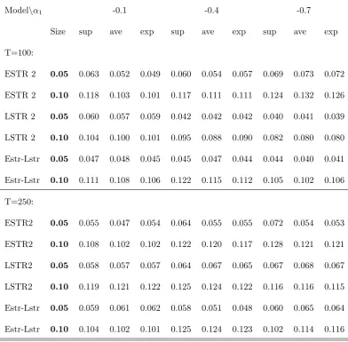
The results in Table 1 show satisfying properties of the test since the simulated p-values are
close to its nominal size for both samples. There are no clear di¤erences between the speci…cations,
although the test tends to overreject slightly against both the models for high values of the linear
adjustment parameter. Supstatistic also slightly overrejects relatively to other two statistics in
the case of exponential model.
Next, the power of the test is examined by specifying the following simple two-variable DGP:
xt=
2 6 6 4 0 B B @ 2 6 6 4 1 3 7 7 5xt l;
1 C C Ad+
3 7 7 5 2 6 6 4 1 3 7 7
5xt 1+ xt 1+ t, =
2 6 6 4
0:54 0:45
0:4 0:45
3 7 7 5.
where diagonal elements of ( ) are given in equations (3) and (4). The errors are again
…rst assumed to be homoscedastic and drawn from the independent N(0;1) distribution. We
…x = 0:2 0
0
, = 1, and reported elements of were chosen randomly such that the
stability condition is satis…ed for the choice ofd.3 The nonlinear adjustment parameter in second
equation is set to (d2 = 0:3) and d1 varies between (-0.1,-0.4,-0.6). The experiment is designed
to capture the power of the test in a less than ideal situation when the adjustment parameters in
one (extreme) regime are small and the adjustment of one of the variables in the second extreme
regime is moderate. Transition parameter 1 vary between(0:1;0:4;0:7;1;2)and we set 2= 0:2.
We do not consider higher values of since they imply that a large portion of data is (or very
close) to one of the extreme regimes, which a¤ects negatively the power of the test and the general
intuition can be inferred from the present choice. The size is set at 5%.
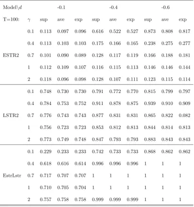
The results from Table 2a and Table 2b show distinct behaviour between the logistic and
exponential speci…cation. The test against ESTR-type nonlinearity has non-negligible power,
which increases when the nonlinearity is stronger (d1is higher), but it falls down with the increase
in the speed of transition 1. This is a consequence of the model speci…cation since the higher
value of 1 implies faster transition between the regimes and more data points at the extremes.
Unless the sample size is large, this will mask the presence of the two regimes’nonlinearity. For
example, when is set to
=
0:7, on average roughly 70% of observations of (Zt 1; )are very close to 1, implying that the system is close to the extreme linear regime. On the other hand, thelogistic speci…cation by de…nition implies a slower rate of transition, although it may su¤er from
identi…cation problems on both ends, which explains the loss of power when !0 and/or when
increases. As increases, the LSTR model becomes closer to threshold speci…cation, where
the data is concentrated at two extremes, although this happens at a much slower rate relative
to ESTR (for
=
0:7, 20 % of observations are close to the extremes). However, contrary toESTR, the LSTR model is subject to identi…cation problems when is close to zero since the
logistic function becomes ‡at and concentrated around1=2, implying the existence of one regime.
This in turn implies that identi…cation of LSTR models and hence ability to direct power against
them also requires a larger number of data points (although the problem is less severe relative to
ESTR), which was also documented in Kristensen and Rahbek (2008).
Four more points are noticeable from the simulation study. First, the power of the test increases
with the sample size and degree of nonlinearity (d1higher), as expected. Second, theaveLMT( )
and expLMT( ) formulations perform better than the sup test for ESTR speci…cation as 1 increases. This is expected since as discussed in Andrews and Ploberger (1994) the former tests
direct power towards alternatives closer to the null, whereas the power of the sup test is with
respect to the distant alternatives. Since the ESTR model for larger values of becomes closer
to the linear speci…cation, the former tests are expected to have a higher power. Third, the test
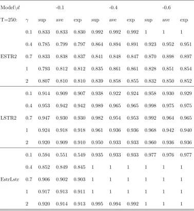
performs relatively well in choosing the correct nonlinear speci…cation. The additional experiment
is performed to illustrate this property of the test. The parameters of the model remain the same,
but the simulated model is now tested against all four possible speci…cations (ESTR-ESTR,
LSTR-LSTR,LSTR-ESTR,ESTR-LSTR) and the number of times the correct speci…cation is selected
given the rejection of linearity is reported in Table 2c. As we can see, the test performs well when
across the variables are present, selecting the correct type of nonlinearity more than90%of times.
The exponential adjustment is correctly selected in at least 80% of cases, where the selection
frequency decreases with the weaker evidence of nonlinearity and/or with the increase in the speed
of transition. This is expected since an ESTR models can be well approximated by an LSTR when
a large portion of observations is close to the upper (extreme) regime since then only the increasing
part of the transition function becomes relevant and hence closer to the monotonically increasing
logistic function. However, as discussed in previous section, the power of the test in such situations
is lower, decreasing the probability of selecting the LSTR model. The experiment thus implies
that in practice one should be relatively con…dent to run the test under di¤erent alternatives and
to choose the one which minimizes the p-value of the test. Fourth, the presence of conditional
heteroscedasticity in one of the series does not signi…cantly deteriorate the size of the test. The
simulation results available from the author show that the size of the test remains close to the
reported one in Table 1 for the range of ARCH(1) speci…cations in one of the residual series.
Next, we investigate the test properties under conditional heteroscedasticity in both residual
series. The mean parameters remain unchanged and we specify the conditional variance as a
simple diagonal BEKK ARCH (1) process:
tjt 1=A00A0+A01 t 1 0t 1A1,
where the parameter matrices are set as A0 = 2 6 6 4
1 0
0:5 1
3 7 7
5 and A1 = 2 6 6 4
a 0
0 a
3 7 7
5 and we
vary a 2[0:2;0:5;0:9]. We perform the experiment over the slightly restricted set of parameter
values(d1; 1)compared to the previous experiment due to high dimensionality, but the results are
general enough to capture the main intuition. We consider the sample size T =250, since it can be
expected that for smaller samples in practice ARCH will not be present (corresponding to quarterly
frequency). P-values are obtained by resampling the estimated residuals from the linear VECM
and creating a new set of residuals B
t = et t, where t v N (0;1). The bootstraped residuals
estimates for each resampled data where p-values are again obtained as the percentage of times
the bootstrap statistics exceeds the sample statistic.
The results in Table 3 and 4 show that the robust LM statistic possess good properties in the
presence of multivariate ARCH volatility. When the level of volatility persistence is moderate,
the empirical size is close to the signi…cance level for exponential model, but it tends to slightly
underreject the null hypothesis in the case of the LSTR model. On the other hand, for large values
ofa= 0:9, size distortions are larger in the case of the ESTR model, where thesupstatistic tends
to overreject more relative to other two statistics.
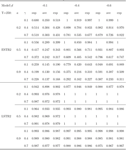
The power of the test remains slightly a¤ected relative to the white noise case. The power
to reject linearity in favour of LSTR nonlinearity remains high and decreases slowly only when
the nonlinearity parameters are small (d1 = 0:1). The power against exponential nonlinearity
decreases more with the level of persistence in ARCH speci…cation. The supstatistic dominates
other two statistics in terms of power against the ESTR, although the di¤erence decreases as the
nonlinearity becomes stronger and transition between the regimes faster, similar to the i.i.d. case.
5
An Application
The presence of smooth type nonlinearity in behaviour of the real exchange rate was heavily
in-vestigated over the past decade, as documented by Taylor and Taylor (2004). However, little was
progressed in examining whether the nonlinearity is present in the relationship between the
nom-inal exchange rate and macro fundamentals and whether this can help in solving a long-standing
puzzle in international economics related to the lack of strong empirical evidence on the
rela-tionship between ‡oating exchange rates and a set of underlying macroeconomic variables. Even
though theories of the exchange rate determination imply that the exchange rate is determined
by such fundamental variables, the empirical evidence on the existence of the relationship and/or
predictability of the future changes in exchange rate on the basis of fundamentals is still scarce
(Cheung, Chinn and Garzia-Pasqual, 2005).
One possibility is that the deviations of the exchange rate from the fundamentally determined
methods. Thus, even though a stable long-run relationship exists, the short-run dynamics will not
be correctly modeled, which will a¤ect the obtained results. It is well-known that di¤erent types
of nonlinearity may arise in the foreign exchange market due to heterogeneity of agents. Overall,
when the exchange rate is close to its fundamental value the in‡uence of technical analysis and
other types of trading strategies dominates the market. Conversely, when the exchange rate
becomes increasingly misaligned with the fundamentals, the pressure from both policy makers
and agents for returning the exchange rate to the neighborhood of the long-run level becomes
stronger and eventually dominates the market. Taylor and Peel (2000) found signi…cant evidence
of nonlinearity in the deviations from the monetary fundamental equilibrium, showing that the
exchange rate follows near-unit process for small deviations (implying lack of cointegration found
in previous studies), but fast mean-reversion for large departures from the long-run equilibrium.
They used a LST type of the test applied on the implied cointegration residual and their results
are univariate. Given the level of interrelations in macro series, imposing a priori exogenenity may
seem as a strong assumption. We, therefore, consider testing for the presence of nonlinearity in
the system framework, providing at the same time the robustness check of the above results.
We consider a classical monetary model of the exchange rate determination, which implies the
existence of the relationship between the exchange rate, money di¤erential and output di¤erential
between two countries. Monthly data on the nominal exchange rate, monetary aggregate and
industrial production for the United States, the United Kingdom and Japan is collected from
the IMF’s International Financial Statistics for the period 1980-2006. The sample includes 324
observations.
All series are expressed in logarithmic terms and they are …rst checked for a unit root, which,
as expected, shows evidence of the nonstationarity. The VAR is then …t to the data, where the
number of lags is computed using AIC criterion, which implied choosing 4 lags for the United
Kingdom and 5 lags for Japan.4 Johansen’s cointegration test …nds (weak) evidence of the unique
cointegrating vector5 for both countries.
4 Multivariate LM tests were also performed to ensure that VAR residuals are indeed white noise.
5 The results for both unit root tests and Johansen’s cointegration test are not reported in order to save space,
We then apply the test for nonlinearity. We allow for the presence of both types of "usual
suspects" nonlinearity (exponential and logistic) in all variables. Although the logistic speci…cation
is less likely to be present in the exchange rate adjustment due to a lack of theoretical underpinnings
as discussed in section 2, we still consider this as an additional check of both model and test
properties. We consider all possible combinations within the system yielding in total 8 di¤erent
alternatives and results are obtained through the grid search with 60 grid points over the nuisance
transition parameter space to [0;50], and over the delay parameter set between [1;12]. The
p-values are obtained using 1000 i.i.d. bootstrap replications. On the basis of simulation results,
the non-robust statistic was employed given that multivariate ARCH LM test did not …nd an
evidence of ARCH e¤ects and univariate ARCH LM tests showed some evidence of conditional
heteroscedasticity only in the money di¤erential series.
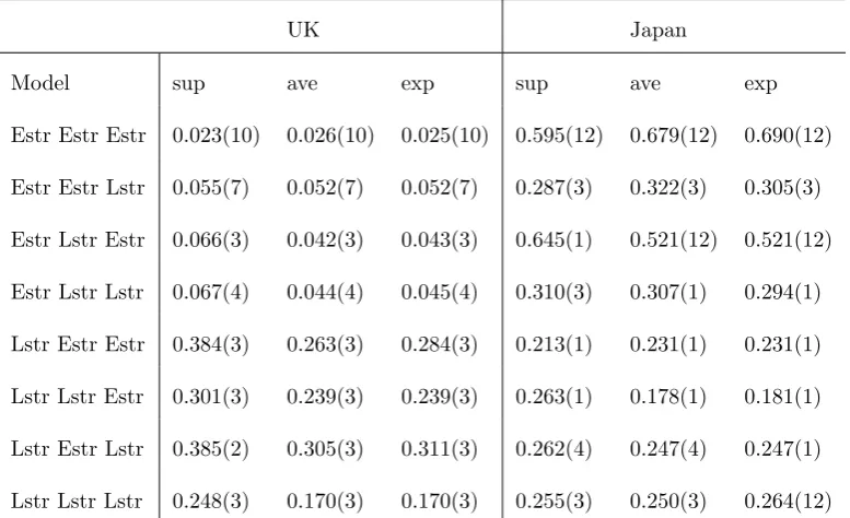
Table 5 shows thep-values from performing all three tests. We only report the minimump-value
per each speci…cation. The number in brackets corresponds to the lagged value of the transition
variable (cointegrating relationship) for which the minimum is attained. As we can see, linearity
is rejected for the monetary model of the British pound using three di¤erent speci…cations, but
the strongest rejection is obtained for the ESTR type nonlinearity in all variables. Following the
evidence from the simulation study, we can be relatively con…dent to conclude that the previously
obtained result by Taylor and Peel (2000) are con…rmed in a more direct way, but, in addition, the
results imply that macro fundamentals also respond in a nonlinear manner to the disequilibrium
in the long-run relationship from 10 months before, where the response in monetary and real
variables depends on the magnitude of over/under pricing of the exchange rate. These links can
be exploited further to investigate whether the evidence of nonlinearity can be used to improve
the forecast of the exchange rate and, at the same time, whether this also helps in predicting
future levels of fundamentals, adding to recently proposed theoretical approach of Engel and West
(2005). On the other hand, no evidence of nonlinearity is found for the Japanese yen, implying
that the nonlinear response in variables is not general and hence the bene…ts of employing the
nonlinear analysis for forecast purposes may di¤er on a country basis. The raised issues warrants
6
Conclusions
In this paper we have proposed a direct test for the presence of nonlinearity in the adjustment terms
of the cointegrating systems that is consistent under the nonlinear alternative. The critical values
are obtained via bootstrap simulations. Monte Carlo simulations show encouraging results in the
presence of homoscedasticity and certain types of heteroscedasticity, but future work is required
to incorporate the broader volatility models, both in terms of the statistical representation of the
nonlinear system and for testing against nonlinearity in such framework.
Another possible extension in both directions is to allow for the richer dependence structure
in the errors of the process. This does not represent a serious de…ciency of the current testing
procedure since choosing the appropriate VAR order will "whiten" the errors. However, once the
progress is made in terms of the Markovian representation of the system under such an assumption,
the changes in the testing procedure would be straightforward using the battery of asymptotic
results for dependent (but not necessarily absolutely regular with geometrically decaying mixing
numbers) processes. The robust type of tests following White (1994) could also be considered in
such framework.
Relaxing the assumption of the known number of cointegrating vectors and testing directly
for it is another fruitful area of research. Some progress has been made for threshold vector
error correction models by Gonzalo and Pitarakis (2006) who proposed the model selection based
approach for determining the rank of the system. In the present context this also requires the "full
representation" proof on the number of nonstationary elements, which is available from Saikkonen
Appendix I: Results:
Table 1: The size of the test:
Modeln 1 -0.1 -0.4 -0.7
Size sup ave exp sup ave exp sup ave exp
T=100:
ESTR 2 0.05 0.063 0.052 0.049 0.060 0.054 0.057 0.069 0.073 0.072
ESTR 2 0.10 0.118 0.103 0.101 0.117 0.111 0.111 0.124 0.132 0.126
LSTR 2 0.05 0.060 0.057 0.059 0.042 0.042 0.042 0.040 0.041 0.039
LSTR 2 0.10 0.104 0.100 0.101 0.095 0.088 0.090 0.082 0.080 0.080
Estr-Lstr 0.05 0.047 0.048 0.045 0.045 0.047 0.044 0.044 0.040 0.041
Estr-Lstr 0.10 0.111 0.108 0.106 0.122 0.115 0.112 0.105 0.102 0.106
T=250:
ESTR2 0.05 0.055 0.047 0.054 0.064 0.055 0.055 0.072 0.054 0.053
ESTR2 0.10 0.108 0.102 0.102 0.122 0.120 0.117 0.128 0.121 0.121
LSTR2 0.05 0.058 0.057 0.057 0.064 0.067 0.065 0.067 0.068 0.067
LSTR2 0.10 0.119 0.121 0.122 0.125 0.124 0.122 0.116 0.116 0.115
Estr-Lstr 0.05 0.059 0.061 0.062 0.058 0.051 0.048 0.060 0.065 0.064
Estr-Lstr 0.10 0.104 0.102 0.101 0.125 0.124 0.123 0.102 0.114 0.116
Table 2a: Power of the test against a speci…c nonlinear alternative:
Modelnd -0.1 -0.4 -0.6
T=100: sup ave exp sup ave exp sup ave exp
0.1 0.113 0.097 0.096 0.616 0.522 0.527 0.873 0.808 0.817
0.4 0.113 0.103 0.103 0.175 0.166 0.165 0.238 0.275 0.277
ESTR2 0.7 0.101 0.090 0.089 0.128 0.117 0.119 0.166 0.188 0.181
1 0.112 0.109 0.107 0.116 0.115 0.113 0.146 0.146 0.144
2 0.118 0.096 0.098 0.128 0.107 0.111 0.123 0.115 0.114
0.1 0.748 0.730 0.730 0.791 0.772 0.770 0.815 0.799 0.797
0.4 0.784 0.753 0.752 0.911 0.878 0.875 0.939 0.910 0.909
LSTR2 0.7 0.776 0.743 0.743 0.877 0.831 0.831 0.865 0.822 0.082
1 0.756 0.723 0.723 0.853 0.812 0.813 0.844 0.814 0.813
2 0.773 0.749 0.748 0.847 0.793 0.793 0.883 0.843 0.843
0.1 0.229 0.233 0.233 0.742 0.733 0.733 0.868 0.862 0.862
0.4 0.618 0.616 0.614 0.996 0.996 0.996 1 1 1
EstrLstr 0.7 0.717 0.707 0.707 1 1 1 1 1 1
1 0.710 0.705 0.704 1 1 1 1 1 1
2 0.757 0.758 0.758 0.999 0.999 0.999 1 1 1
Table 2b: Power of the test (continuation):
Modelnd -0.1 -0.4 -0.6
T=250: sup ave exp sup ave exp sup ave exp
0.1 0.438 0.446 0.447 0.995 0.996 0.995 1 1 1
0.4 0.359 0.385 0.381 0.579 0.628 0.627 0.747 0.819 0.811
ESTR2 0.7 0.355 0.373 0.378 0.458 0.519 0.52 0.530 0.614 0.611
1 0.376 0.396 0.398 0.439 0.475 0.475 0.446 0.508 0.507
2 0.352 0.362 0.364 0.434 0.455 0.457 0.442 0.455 0.456
0.1 0.988 0.987 0.987 0.996 0.995 0.995 0.996 0.996 0.995
0.4 0.999 0.999 0.999 1 0.999 0.999 1 1 1
LSTR2 0.7 0.996 0.994 0.994 1 1 1 1 1 1
1 0.996 0.993 0.993 1 1 1 1 0.999 0.999
2 0.996 0.996 0.996 1 1 1 1 0.999 0.999
0.1 0.467 0.458 0.455 0.983 0.979 0.979 0.998 0.998 0.998
0.4 0.949 0.942 0.941 1 1 1 1 1 1
EstrLstr 0.7 0.984 0.981 0.981 1 1 1 1 1 1
1 0.978 0.978 0.978 1 1 1 1 1 1
2 0.986 0.986 0.986 1 1 1 1 1 1
Table 2c: Empirical frequency of choosing the nonlinear model:
Modelnd -0.1 -0.4 -0.6
T=250: sup ave exp sup ave exp sup ave exp
0.1 0.833 0.833 0.830 0.992 0.992 0.992 1 1 1
0.4 0.785 0.799 0.797 0.864 0.894 0.891 0.923 0.952 0.951
ESTR2 0.7 0.833 0.838 0.837 0.841 0.848 0.847 0.870 0.898 0.897
1 0.793 0.812 0.812 0.835 0.861 0.861 0.828 0.851 0.854
2 0.807 0.810 0.810 0.839 0.858 0.855 0.832 0.850 0.852
0.1 0.914 0.909 0.907 0.938 0.922 0.924 0.958 0.930 0.929
0.4 0.953 0.942 0.942 0.989 0.965 0.965 0.998 0.975 0.975
LSTR2 0.7 0.947 0.930 0.930 0.982 0.954 0.953 0.992 0.964 0.965
1 0.924 0.918 0.918 0.961 0.936 0.936 0.968 0.942 0.940
2 0.920 0.909 0.910 0.950 0.933 0.933 0.960 0.936 0.936
0.1 0.594 0.551 0.549 0.935 0.933 0.933 0.977 0.976 0.977
0.4 0.852 0.849 0.845 1 1 1 1 1 1
EstrLstr 0.7 0.906 0.902 0.903 1 1 1 1 1 1
1 0.917 0.913 0.911 1 1 1 1 1 1
2 0.920 0.914 0.913 0.995 0.994 0.992 1 1 1
Table 3: Size of the test in the presence of ARCH e¤ects:
Modeln -0.1 -0.4
T=250: a size sup ave exp sup ave exp
0.2 0.05 0.060 0.055 0.059 0.073 0.071 0.074
0.2 0.10 0.094 0.112 0.101 0.141 0.123 0.128
ESTR2 0.5 0.05 0.058 0.055 0.053 0.064 0.055 0.060
0.5 0.10 0.116 0.105 0.108 0.115 0.114 0.112
0.9 0.05 0.082 0.071 0.070 0.070 0.051 0.066
0.9 0.10 0.138 0.110 0.114 0.148 0.114 0.130
0.2 0.05 0.040 0.033 0.033 0.033 0.029 0.030
0.2 0.10 0.082 0.073 0.073 0.067 0.063 0.063
LSTR2 0.5 0.05 0.052 0.045 0.045 0.025 0.028 0.028
0.5 0.10 0.079 0.076 0.077 0.067 0.059 0.060
0.9 0.05 0.042 0.041 0.040 0.055 0.046 0.047
0.9 0.10 0.088 0.072 0.071 0.101 0.086 0.085
‘
Table 4: Power of the test in the presence of ARCH e¤ects:
Modelnd -0.1 -0.4 -0.6
T=250: a sup ave exp sup ave exp sup ave exp
0.1 0.680 0.350 0.518 1 0.919 0.997 1 0.999 1
0.2 0.4 0.514 0.304 0.428 0.898 0.704 0.833 0.982 0.914 0.970
0.7 0.518 0.303 0.431 0.781 0.535 0.677 0.879 0.726 0.822
0.1 0.556 0.289 0.399 1 0.850 0.984 1 0.994 1
ESTR2 0.5 0.4 0.417 0.247 0.343 0.801 0.566 0.711 0.931 0.807 0.893
0.7 0.372 0.242 0.317 0.609 0.405 0.542 0.796 0.617 0.747
0.1 0.259 0.145 0.190 0.779 0.420 0.643 0.948 0.691 0.889
0.9 0.4 0.199 0.130 0.156 0.375 0.216 0.310 0.591 0.387 0.509
0.7 0.228 0.137 0.168 0.292 0.162 0.227 0.387 0.233 0.311
0.1 0.942 0.898 0.902 0.977 0.946 0.949 0.988 0.977 0.978
0.2 0.4 0.993 0.976 0.978 1 1 1 1 1 1
0.7 0.987 0.972 0.972 1 1 1 1 1 1
0.1 0.964 0.933 0.935 0.993 0.980 0.981 0.995 0.984 0.986
LSTR2 0.5 0.4 0.982 0.969 0.972 1 1 1 1 1 1
0.7 0.991 0.978 0.979 1 1 1 1 1 1
0.1 0.993 0.986 0.987 0.997 0.995 0.995 0.998 0.998 0.998
0.9 0.4 0.989 0.980 0.982 0.991 0.988 0.988 0.985 0.981 0.981
0.7 0.987 0.977 0.977 0.988 0.986 0.986 0.975 0.967 0.967
Table 5: Testing the monetary model of exchange rates:
UK Japan
Model sup ave exp sup ave exp
Estr Estr Estr 0.023(10) 0.026(10) 0.025(10) 0.595(12) 0.679(12) 0.690(12)
Estr Estr Lstr 0.055(7) 0.052(7) 0.052(7) 0.287(3) 0.322(3) 0.305(3)
Estr Lstr Estr 0.066(3) 0.042(3) 0.043(3) 0.645(1) 0.521(12) 0.521(12)
Estr Lstr Lstr 0.067(4) 0.044(4) 0.045(4) 0.310(3) 0.307(1) 0.294(1)
Lstr Estr Estr 0.384(3) 0.263(3) 0.284(3) 0.213(1) 0.231(1) 0.231(1)
Lstr Lstr Estr 0.301(3) 0.239(3) 0.239(3) 0.263(1) 0.178(1) 0.181(1)
Lstr Estr Lstr 0.385(2) 0.305(3) 0.311(3) 0.262(4) 0.247(4) 0.247(1)
Lstr Lstr Lstr 0.248(3) 0.170(3) 0.170(3) 0.255(3) 0.250(3) 0.264(12)
Appendix II: Proofs
To keep exposition simpler, all proofs are stated for the case of conditional homoscedasticity, but
can be easily amended using the triangular inequality to include permitted classes of conditionally
heteroscedastic models under the existence of higher moments of the error process and using the
facts that the processHtis stationary, ergodic with …nite moments and that Ht(Ht0Ht) 1Ht t0
k tk by the standard result for projection matrices. In the following to save space Pt =
PT t=1 andK is a generic constant.
Proof of Proposition 1.1. Consider …rst expression within the norm. Since Zt0 1Zt 1 is a scalar term and (Zt 1; ) = (Zt 1; )0, this can be rearranged as follows:
jj 0
t
1
Z0
t 1 (Zt 1; ) jj= tr n
0
t
1
Z0
t 1 (Zt 1; ) Zt 1 (Zt 1; ) 1
0
t
o 1 2
= trn 0
t
1
Z0
t 1Zt 1 (Zt 1; ) (Zt 1; ) 1
0
t
o 1 2
= trnZ0
t 1Zt 1 0t
1
(Zt 1; ) (Zt 1; ) 10 t
o 1 2
= Z0
t 1Zt 1
1 2 trn 0
t
1
(Zt 1; ) (Zt 1; ) 10 t
o 1 2
jj 0t
1
Zt0 1 (Zt 1; ) jj2+ =jjZt 1jj2+ jj (Zt 1; ) 1
0
tjj
2+
Substituting back into expression and using the Cauchy-Schwarz (C-S) inequality:
Ehsup 2 jj 0
t
1
Z0
t 1 (Zt 1; ) jj 2+ i
=EhjjZt 1jj2+ sup 2 jj (Zt 1; ) 1
0
tjj
2+ i
EjjZt 1jj2(2+ )
1 2
Esup 2 jj (Zt 1; ) 1
0 tjj 2(2+ ) 1 2 (9)
Boundness of the …rst term in (10) now follows from Assumptions 1.1 and 1.2 given the existence
of moments of the Markov chain and choosing arbitrarily. Consider the second term:
jj (Zt 1; ) 1
0
tjj
2+
= trn 1 (Z
t 1; ) (Zt 1; ) 10
t 0t
o 1 2(2+ )
By Hölder’s inequality for matrices (Magnus and Neudecker, 2007, pp. 250), wheresis slightly
higher than 1 andqis large:
trn 1 (Z
t 1; ) (Zt 1; )
10 so 12 (2+ )
s
tr (0
t t) q
1 2
(2+ )
q
= trn 1 (Z
t 1; ) (Zt 1; )
10 so 12 (2+ )
s
( 0
t t) q
1 2
(2+ )
q
= trn 1 (Z
t 1; ) (Zt 1; )
10 so
1 2
(2+ )
s
( 0
t t)
1 2(2+ )
Ehsup 2 jj 0
t
1
Z0
t 1 (Zt 1; ) jj 2+ i
K1 E "
sup 2 trn 1 (Z
t 1; ) (Zt 1; )
10 so 12 (2+ )
s
jj tjj2(2+ )
#!1 2
Given the independence of errors, constancy of the error’s covariance matrix and boundness of
(Zt 1; )between[0; r], Proposition 1.1. then follows provided thatsuptEjj tjj2(2+ )is bounded,
which follows from Assumption 1.1. choosing arbitrarily.
Proof of Proposition 1.2. First we will show su¢ cient condition to satisfy the Proposition
and then prove that the condition is satis…ed in current model. Set = 2+1 and similarly to the
proof of Proposition 2.1. rearrange the norm using properties of trace of the Kronecker product:
jj 0
t
1
Z0
t 1 ( (Zt 1; 1) (Zt 1; )) jj 2+
=
=jjZt 1jj2+ jj 0t 1 (Zt 1; 1) (Zt 1; ) jj2+ (10)
Consider only the second norm. By the mean value theorem for 2[ ; 1], Hölder’s inequality6
for matrices withsslightly higher than 1 andqlarge:
jj 0t 1 Ik vec (Zt 1; 1) (Zt 1; ) jj 2+
=jj 0t 1 Ik 5 (Zt 1; ) ( 1 )jj 2+
= tr 5 (Zt 1; )0 10 t 0t 1 Ik 5 (Zt 1; ) ( 1 )( 1 )0
1 2(2+ )
trn 5 (Zt 1; )0 10 t 0t 1 Ik 5 (Zt 1; )
so 21s(2+ )
trn ( 1 )0( 1 ) qo
1 2q(2+ )
= trn 5 (Zt 1; )0 10 t 0t 1 Ik 5 (Zt 1; )
so 21s(2+ )
( 1 )0( 1 )
1 2(2+ )
De…ne the …rst term above as (Zt 1; ), such that we can write:
jj 0t 1 (Zt 1; 1) (Zt 1; ) )jj 2+
= (Zt 1; )jj( 1 )jj 2+
(11)
Substituting (11) in (10) and using (10) the condition can be expressed as:
suptEhjjZt 1jj2+ sup
12 :jj 1 jj<$ (Zt 1; )jj( 1 )jj
2+ i
6 Note that Hölder’s inequality holds only for positive semi-de…nite matrices of the same order. 5 (Zt 1; )0 10 t t0 1 Ik 5 (Zt 1; ) is positive de…nite since by construction (k
2 x kr) matrix
5 (Zt 1; )is of full column rank and positive de…niteness of the middle term follows from Assumption 1.1.
suptEhjjZt 1jj2+ sup 2 (Zt 1; ) i
$2+
Hence, Proposition 1.2. follows by setting = 2+1 (2 + ) = 1 and choosing C arbitrarily
provided thatsuptE
h
jjZt 1jj2+ sup 2 (Zt 1; ) i
<1
By C-S inequality boundness of the …rst term again follows from assumptions 1.1 and 1.2:
suptEhjjZt 1jj2+ sup 2 (Zt 1; ) i
supt EjjZt 1jj2(2+ )
1 2
Ejsup 2 (Zt 1; )j2
1 2
K2supt E sup 2 tr
n
5 (Zt 1; )0 10 t 0t 1 Ik 5 (Zt 1; )
so 21s(2+ )
2!12
Using the fact that the Frobenius norm is always positive and rearranging:
=K2supt Esup 2 tr
n 10
t 0t 1 Ik 5 (Zt 1; )5 (Zt 1; )0
so 21s(2+ )2
1 2
Applying the Hölder’s inequality with wslightly higher than 1 andmlarge:
K2supt
0 B B @
E tr 10
t 0t 1 Ik
sw 1 2sw(2+ )2
sup 2 trn 5 (Zt 1; )5 (Zt 1; )0
smo 2sm1 (2+ )2
1 C C A 1 2
Using Assumption 1.4. and after that Assumption 1.1 and properties of the Kronecker product,
it follows that:
K2supt E
h
tr 10
t 0t 1 Ik
sw 2sw1 (2+ )2
K3 Zt0 1Zt 1
sm 2sm1 (2+ )2i
1 2
=K4supt E
h
tr 10
t 0t 1
sw 1 2sw(2+ )2
jjZt 1jj(2+ )2 i 1
2
=K4supt E tr t 0t 1 10
sw 1 2sw(2+ )2
1 2
EjjZt 1jj(2+ )2
1 2
where the last line follows from the error independence assumption. The boundness of the …rst
term above now follows using Assumption 1.1, while the boundness of the second term follows
from assumptions 1.1. and 1.2.
Proof of Proposition 2. First, note that due to superconsistency of e:
1
p
T
P
t 0t
1
Z0
t 1(e) (Zt 1(e); ) =p1T Pt 0t
1
Z0
t 1 (Zt 1; ) +op(1)and in the
remaining part of the proof only the score evaluated atZt 1 is considered.
The proof follows by verifying the …nite dimensional (…di) convergence ofsfT( )and stochastic
equicontinuity of the empirical process. Both follow from the Theorem 1 Application 1 of DMR
(1995). First note that choosing (x) =x1+2, x >0, in DMR it can be shown (Cho and White,
2007, pp.1705) that condition (2.9a) in Lemma 2 of DMR will be satis…ed for -mixing processes
with geometrically decaying numbers. Lemma 2 of DMR then implies that the conditions on
with respect to thek k2(1+
2) =k k2+ norm instead of thek k2; norm proposed in their paper.
Fidi convergence then follows from Theorem 1 of DMR given the Assumption 1.2, if the class
of functions zof the empirical process belongs to the class whose envelope has bounded 2 +
moments. Proposition 1.1. ensures that the condition is satis…ed in our case.
Furthermore, condition (2.4) in DMR on summability of -mixing coe¢ cientsPt nis trivially satis…ed by Assumption 1.2. on the rate of mixing numbers: Pt n=PtCbnand since0< b <1
= C1bb < 1: It remains to show that the entropy with bracketing satis…es the integrability condition (2.11) in DMR. This follows from Theorem 5 in Andrews (1994, see also Andrews, 1993,
pp.201) if theLp-continuity condition holds which is established in Proposition 1.2. forp= 2 + .
Proof of Proposition 3. By triangular inequality:
sup 2 VeT( ) V( ) sup 2 VeT( ) VT( ) + sup 2 jjVT( ) V( )jj
Start with the second term on the right hand side, where the uniform convergence of VT( )
over 2 is established. Note that under the null hypothesis and Assumptions 1.1 and 1.2.
pointwise convergence for each follows from the ergodic theorem since all elements of VT( ) =
1
T
P
tZt 1Zt0 1 t 1( ) 1 t 1( ) are strictly stationary and mixing sequences and hence ergodic sequences (Proposition 3.44 in White, 2001). The convergence follows given the existence
of suitable moments, which follows from Assumptions 1.1 and 1.2. We then need to establish
conditions under whichVT( )is stochastically equicontinious over 2 and uniform convergence
follows from Theorem 2.1 in Newey (1991). VT( ) V( )is stochastic equicontinious over in
the sense that:
suptPhsup 2 sup
12B( ;$)jjVT( ) V( 1)jj>
i p
!0;as
$
!0,where B( ;
$
)is a ball of radius$
around :k 1k$
By Markov’s inequality:
1 sup
t
E
"
sup
2
sup
12B( ;$)
jjVT( ) V( 1)jj #
(12)
= T1 PtZt 1Zt0 1 t 1( ) 1 t 1( ) t 1( 1) 1 t 1( 1) 1
T
P
t Zt 1Zt0 1 t 1( ) 1 t 1( ) t 1( 1) 1 t 1( 1)
sup
t
Zt 1Zt0 1 t 1( ) 1 t 1( ) t 1( 1) 1
t 1( 1) (13)
Using the fact that trfA Cg =trfAgtrfCg and that Z0
t 1Zt 1 is a scalar term, this can be rearranged as:
= suptkZt 1k2 t 1( ) 1 t 1( ) t 1( 1) 1 t 1( 1) Since(trfA0Ag)1=2= vecA0vecA 1=2:
= suptkZt 1k2 vec t 1( ) 1 t 1( ) vec t 1( 1) 1 t 1( 1)
By the mean value theorem for vector functions (Magnus and Neudecker, 2007, pp.110) and
for 2[ ; 1]
= suptkZt 1k2 Ik t 1( ) 1 r t 1( )( 1) + t 1( )
0 1
Ik r t 1( )( 1)
= sup
t
sup
2 k
Zt 1k2 Ik t 1( ) 1+ t 1( )
0 1
Ik r t 1( )( 1) (14)
where r t 1( )is(k2xkr)matrix of partial derivatives for some 2[ ; 1]. De…ne C( ) =Ik t 1( ) 1+ t 1( )
0 1
Ik and note that (12) is majorized by 1sup
tE
h
kZt 1k2sup 2 sup 12B( ;$) C( )r t 1( )( 1) i
By the C-S inequality:
1sup
t EkZt 1k4
1 2
E sup 2 sup
12B( ;$) C( )r t 1( )( 1)
2 12
Given the Assumptions 1.1. and 1.2. supt EkZt 1k4 <1, such that by the positiveness of the Frobenius norm:
1K
5supt E sup 2 sup 12B( ;$) C( )r t 1( )( 1)
2 12
= 1K5supt Esup 2 sup 12B( ;$) C( )r t 1( )( 1)
2 12
By repeated application of the Hölder’s inequality7 withs; w slightly higher than 1 andqand
mlarge:
7 Note thatC( )has full rank given the Assumption 1.1. using the fact that rank(A B) =rank(A)rank(B).
1K
5supt(E[ sup 2 sup 12B( ;$) tr
n
C( )0C( ) qo
2 2q
trn ( 1)( 1)0r t 1( )0r t 1( )
so 22s
])12
1K
5supt(E[ sup 2 sup 12B( ;$) tr
n
C( )0C( ) qo
2 2q
trn ( 1)( 1)0 smo
2 2sm
trn r t 1( )0r t 1( )
swo 2sw2
])12
= 1K5supt(E[ sup 2 sup 12B( ;$) tr
n
C( )0C( ) qo
1
q
k 1k
2
trn r t 1( )0r t 1( )
swo 2sw2
])12
Using Assumption 1.4. and rearranging:
$K
5supt E sup 2 tr
n
C( )0C( ) qo
1
q
Z0
t 1Zt 1
sw 2 2sw
1 2
Since C( ) consists of elements which are constant and bounded between zero and one,
sto-chastic equicontinuity follows by letting
$
!0 under assumptions 1.1 and 1.2. which establishboundness of the last term.
It remains to show that the …rst term is op(1) uniformly in . This follows easily under
Assumption 1.3. after taking into account di¤erent rates of convergence in the long-run and
short-run parameters as in Saikkonen (1995).
sup 2 VeT( ) VT( ) =
sup
2
1
T
P
tZt 1(e)Z0t 1(e) t 1(e; )e 1 t 1(e; ) 1
T
P
tZt 1( 0)Z0t 1( 0) t 1( 0; ) 1 t 1( 0 )
(15)
By triangular inequality (15) can be rearranged as:
sup 2 T1PtpT(e )0p1
TX2;t 1
1
p
TX
0
2;t 1
p
T(e ) t 1(e; )e 1 t 1(e; ) +sup 2 T1Pt
p
T(e )0p1
TX2;t 1Z
0
t 1( 0) t 1(e; )e 1 t 1(e; ) +sup 2 T1 PtZt 1( 0)p1TX20;t 1
p
T(e ) t 1(e; )e 1
t 1(e; )
+ sup 2 T1 PtZt 1( 0)Z0t 1( 0) t 1(e; ) t 1( 0; ) e 1 t 1(e; )
+ sup 2 T1 PtZt 1( 0)Z0t 1( 0) t 1( 0; )e 1 t 1(e; ) t 1( 0; )
+ sup 2 T1 PtZt 1( 0)Z0t 1( 0) t 1( 0; ) e 1 0 1 t 1( 0; ) Now we need to show that each term isop(1).