Predictive density accuracy tests

(1)

WORKING PAPERS SERIES

WP04-16

(2)

Predictive Density Accuracy Tests

∗

Valentina Corradi1 _{and Norman R. Swanson}2

1_{Queen Mary, University of London and} 2_{Rutgers University}

February 2004

Abstract

This paper outlines a testing procedure for assessing the relative out-of-sample predictive accuracy of multiple condi-tional distribution models, and surveys existing related methods in the area of predictive density evaluation, including methods based on the probability integral transform and the Kullback-Leibler Information Criterion. The procedure is closely related to Andrews’ (1997) conditional Kolmogorov test and to White’s (2000) reality check approach, and involves comparing square (approximation) errors associated with modelsi, i= 1, ..., n,by constructing weighted

averages overU ofE!"Fi(u|Zt,θ†i)−F0(u|Zt,θ0)

#2$

,whereF0(_·|·) and Fi(·|·) are true and approximate

distributions, u ∈ U, and U is a possibly unbounded set on the real line. Appropriate bootstrap procedures for obtaining critical values for tests constructed using this measure of loss in conjunction with predictions obtained via rolling and recursive estimation schemes are developed. We then apply these bootstrap procedures to the case of obtaining critical values for our predictive accuracy test. A Monte Carlo experiment comparing our bootstrap methods with methods that do not include location bias adjustment terms is provided, and results indicate coverage improvement when our proposed bootstrap procedures are used. Finally, an empirical example comparing alternative predictive densities for U.S. inflation is given.

JEL classification: C22, C51.

Keywords: block bootstrap, rolling and recursive estimation scheme, parameter estimation error, predictive density.

∗ _{Valentina Corradi, Department of Economics, Queen Mary, University of London, Mile End Road, London E1}

(3)

1 Introduction

In the management of financial risk in the insurance and banking industries, there is often a need for examining confidence intervals or entire conditional distributions. One such case is when value at risk measures are constructed in order to assess the amount of capital at risk from small probability events, such as catastrophes (in insurance markets) or monetary shocks that have large impact on interest rates (see Duffie and Pan (1997) for further discussion). These considerations in part account for the development over the last few years of a new strand of literature addressing the issue of predictive density evaluation. Some of the important recent papers in this area include Diebold, Gunther and Tay (DGT: 1998), Christoffersen (1998), Bai (2003), Diebold, Hahn and Tay (1999), Hong (2001) and Christoffersen, Hahn and Inoue (2001), and Giacomini (2002).1 _This paper has two primary objectives. First, we build on the results of Corradi and Swanson (2003a) by outlining a procedure for assessing the relative out-of-sample predictive accuracy of multiple conditional distribution models that can be used with rolling and recursive estimation schemes. Second, we provide a brief survey of related techniques, such as those based on the use of the probability integral transform and the Kullback-Leibler Information Criterion (KLIC).

The literature on the evaluation of predictive densities is largely concerned with testing the null of correct dynamic specification of an individual conditional distribution model. However, in the literature on the evaluation of point forecast models it is acknowledged that all models in a group that is being evaluated may be misspecified (see e.g. White (2000) and Corradi and Swanson (2002)). In this paper, we draw on elements of these two literatures in order to provide a test for choosing among a group of misspecified out-of-sample predictive density models. Reiterating our above point, the focus of most of the papers cited above is that the density associated with the true conditional distribution is clearly the best predictive density. Therefore, evaluation of predictive densities is usually performed via tests for the correct (dynamic) specification of the conditional distribution. Along these lines, by making use of the probability integral transform, DGT suggest a simple and effective means by which predictive densities can be evaluated. Using the DGT terminology, if pt(yt|Ωt−1) is the “true” conditional distribution of yt|Ωt−1,then pt(yt|Ωt−1) is an

1_{Ten years ago, when Clive Granger was asked by one of the authors of this paper in an interview what he thought}

the most important future areas in time series analysis were, he replied that predictive density construction and

(4)

identically and independently distributed uniform random variable on [0,1]; so that the difference between an empirical version of pt(yt|Ωt−1) constructed using estimated parameters and the 45 degree line can be used as measure of goodness of fit.2 _{A feature common to the papers cited} above is that the null hypothesis is that of (dynamic) correct specification. Our approach differs from these as we do not assume that any of the competing models (including the benchmark) are correctly specified.3 _{Thus, we posit that} _all _{models should be viewed as approximations of some} true unknown underlying data generating process. For this reason, it is our objective in this paper to provide a conditional Kolmogorov test, in the spirit of Andrews (1997), that allows for the joint comparison of multiple misspecified conditional distribution models, for the case of dependent observations. In particular, assume that the object of interest is the conditional distribution of a scalar, Yt+1,given a (possibly vector valued) conditioning set, Zt, where Zt contains lags of Yt+1 and/or lags other variables. Now, given a group of (possibly) misspecified conditional distributions,

F1(u_|Zt,θ†₁), ..., Fm(u|Zt,θ†m), assume that the objective is to compare these models in terms of

their closeness to the true conditional distribution, F0(u|Zt,θ0) = Pr(Yt+1 ≤ u|Zt). If m > 2, we follow White (2000), in the sense that we choose a particular conditional distribution model as the “benchmark” and test the null hypothesis that no competing model can provide a more accurate approximation of the “true” conditional distribution, against the alternative that at least one competitor outperforms the benchmark model. However, unlike White, we evaluate predictive densities rather than point forecasts. Needless to say, pairwise comparison of alternative models,

2_{Using the same approach, Bai (2003) proposes a Kolmogorov type test based on the comparison of}_p

t(yt|Ωt−1,θT) with the CDF of a uniform on [0,1].As a consequence of using estimated parameters, the limiting distribution of

his test reflects the contribution of parameter estimation error and is not nuisance parameter free. To overcome this

problem, Bai (2003) uses a novel device based on a martingalization argument to construct a modified Kolmogorov

test which has a nuisance parameter free limiting distribution. His test has power against violations of uniformity but

not against violations of independence. Hong (2001) proposes an interesting test, based on the generalized spectrum,

which has power against both uniformity and independence violations, for the case in which the contribution of

parameter estimation error vanishes asymptotically. For the case where the null is rejected, Hong (2001) also proposes

a test for uniformity that is based on a comparison between a kernel density estimator and the uniform density,

and that is robust to non independence (see also Hong and Li (2003)). Diebold, Hahn and Tay (1999) propose a

nonparametric correction for improving the density forecast when the uniform (but not the independence) assumption

is violated. Finally, Bontemps and Meddahi (2003a,b) suggest a GMM type approach for testing normality and various

distributional assumptions.

(5)

in which no benchmark need be specified, follows from our results as a special case. In our context, accuracy is measured using a distributional analog of mean square error. More precisely, the squared (approximation) error associated with modeli, i= 1, ..., m,is measured in terms of the average over

U of E!"Fi(u|Zt+1,θ†i)−F0(u|Zt+1,θ0)

#2$

,whereu_∈U, and U is a possibly unbounded set on the real line.4 _{It should be pointed out that one well known measure of distributional accuracy is} the Kullback-Leibler Information Criterion (KLIC), in the sense that the “most accurate” model can shown to be that which minimizes the KLIC (see Section 2 for a more precise discussion). Using the KLIC approach, Giacomini (2002) suggests a weighted version of the Vuong (1989) likelihood ratio test for the case of dependent observations, while Kitamura (2002) employs a KLIC based approach to select among misspecified conditional models that satisfy given moment conditions.5 _{Furthermore, the KLIC approach has been recently employed for the evaluation of} dynamic stochastic general equilibrium models (see e.g. Sch¨orfheide (2000), Fernandez-Villaverde and Rubio-Ramirez (2001), and Chang, Gomes and Sch¨orfheide (2002)). For example, Fernandez-Villaverde and Rubio-Ramirez (2001) show that the KLIC-best model is also the model with the highest posterior probability. In general, there is no reason why our measure of accuracy is more “natural” than the KLIC, or vice-versa. However, in the next section we outline how certain problems (such as comparing conditional confidence intervals) that are difficult to address using the KLIC can be handled quite easily using our measure of distributional accuracy.

The limiting distribution of the suggested statistic turns out to be a functional of a Gaussian process with a covariance kernel reflecting both (dynamic) misspecification and parameter estima-tion error (PEE). The limiting distribuestima-tion is not nuisance parameter free and critical values cannot be directly tabulated. Valid asymptotic critical values can be obtained via an empirical version of the block bootstrap which properly takes into account PEE, however. The PEE contribution is summarized by the limiting distribution of P−1/2%_tT₌−_R1"θ&t−θ†

#

,where R denotes the length of the estimation period, P the number of recursively estimated parameters, θ&t is either a recursive

m−estimator constructed using the firsttobservations or a rollingm−estimator constructed using

observations from t−R+ 1 to t, and θ† is its probability limit. Intuitively, in the recursive case,

4_{To the best of our knowledge, the only other papers in which this measure is considered are Corradi and Swanson}

(2003a,b).

5_{Of note is that White (1982) shows that quasi maximum likelihood estimators (QMLEs) minimize the KLIC,}

(6)

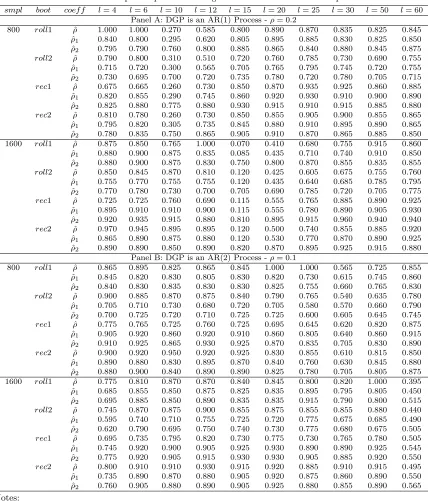
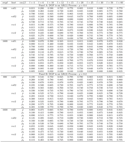
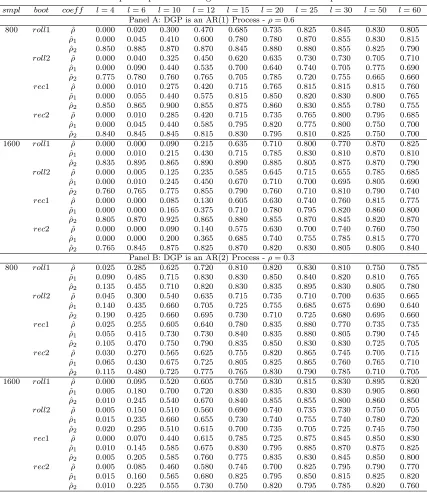
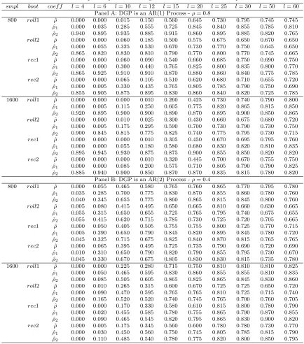
earlier observations are used more frequently than temporally subsequent observations, while in the rolling case, observations in the center of the sample are used more frequently than observa-tions either at the beginning or at the end of the sample. This introduces a location bias to the usual block bootstrap, as under standard resampling with replacement schemes, any block from the original sample has the same probability of being selected.6 _{We consider two solutions to this} problem. First, we modify the usual resampling scheme and add an adjustment term which corrects for the bootstrap location bias. Second, we retain the usual resampling scheme, but add additional adjustment terms to those needed when our modified resampling scheme is used. Additionally, we consider cases in which all parameters are jointly estimated as well as cases where the conditional mean parameters are first estimated via OLS or NLS, and the error variance is subsequently es-timated using the residuals from the conditional mean model.7 _{In order to assess the usefulness} of our bootstrap procedures, we carry out a series of Monte Carlo experiments evaluating finite sample coverage probabilities of our “PEE” bootstraps for rolling and recursive estimation schemes with analogous bootstrap methods that do not include our “adjustment” terms. Results indicate that the adjustment terms lead to improved coverage probabilities. Thus, our procedures should prove useful for constructing critical values for our predictive density accuracy tests.

The rest of the paper is organized as follows. Section 2 outlines the setup, presents the predictive density accuracy test, and states the asymptotic properties of the test statistic for both the case of recursive and rolling parameter estimation schemes. Section 3 is broken into four subsections. The first two subsections outline bootstrap procedures for mimicking the limiting distribution of parameter estimation error in rolling estimation schemes, while the third subsection summarizes the results of Corradi and Swanson (2003a) for recursive estimation schemes. Finally, the fourth subsection applies the results of the previous two subsections in order to obtain asymptotically valid critical values for the predictive density accuracy test. Section 4 contains the results of a

6_{Note that in the fixed sampling scheme, we just need to take into account the contribution of}√_R _θ

R−θ† , whose limiting distribution is properly captured by “standard” block bootstrap techniques, using for example the

results of Goncalves and White (2003). This case has been considered by Corradi and Swanson (2003b), within the

context of in sample evaluation of conditional misspecified distribution models.

7_{From a theoretical perspective, it should be noted that all of our rolling estimation scheme results are new}

to this paper. Additionally, our recursive estimation scheme results for the case where parameters are estimated

sequentially are new, while those for the joint estimation case summarize previous results reported in Corradi and

(7)

small Monte Carlo study of the bootstrap procedures developed in the paper, in particular (i) we compare the relative coverage probabilities for recursive and rolling schemes, and (ii) we evaluate the importance of the adjustment term in our bootstrap. In Section 5, an empirical example based on predicting U.S. inflation is presented. Finally, concluding remarks are gathered in Section 6. All proofs are in an appendix. Hereafter, P∗ denotes the probability law governing the resampled series, conditional on the sample,E∗andV ar∗the mean and variance operators associated withP∗, o∗_P(1) Pr−P denotes a term converging to zero inP∗−probability, conditional on the sample except

a subset of probability measure approaching zero, and finallyO∗_P(1) Pr−P denotes a term which is bounded in P∗−probability, conditional on the sample except a subset of probability measure

approaching zero.

2 Predictive Density Evaluation

Our objective is to “choose” a conditional distribution model that provides the most accurate out-of-sample approximation of the true conditional distribution, given multiple predictive densities, and allowing for misspecification under both the null and the alternative hypotheses. One strategy that yields tests of the null of correct specification that are equally as useful as those discussed above is the conditional Kolmogorov test approach of Andrews (1997), which is based on a direct compar-ison of empirical joint distributions with the product of parametric conditional and nonparametric marginal distributions. Corradi and Swanson (2003c) extend Andrews (1997) in order to allow for the in-sample comparison of multiple misspecified models. As discussed above, one of our main objectives in this paper is the extension of those results to out-of-sample predictive density eval-uation in the context of various different estimation schemes. From the perspective of prediction, we assume that the objective is to form parametric conditional distributions for a scalar random variable, yt+1, given Zt, and to select among these, where Zt = (yt, ..., yt−s1+1, Xt, ..., Xt−s2+1),

t = s, ...,T , ...' T'+s, with s = max_{s1, s2}, and T'+s = T, with T = (s+R) +P. Assume that

i= 1, ..., n different models are estimated. In order to examine rolling estimation schemes, define therolling m-estimator for the parameter vector associated with model ias:

&

θi,t,R= arg max

θi∈Θi

1 R

t

(

j=t−R+1

(8)

and

θ_i†= arg max

θi∈Θi

E(lnfi(yj, Zj−1,θi)), (2)

where fi(·|·,θi) is the conditional density associated with Fi(·|·), i = 1, ..., n, so that θi† is the

probability limit of a quasi maximum likelihood estimator (QMLE).If modeliis correctly specified, thenθ†_i =θ0.We compute a sequence aP estimators, first using observations froms+ 1 to R+s, then from tos+ 2 to R+s+ 1,and so on until we use the lastR observations, that is fromP+s to T−1. These estimators are then used to construct sequences of P 1-step ahead forecasts and associated forecast errors, for example. In the context of such rolling estimators, it is necessary to distinguish between the cases of P ≤ R and P > R, as we shall see below. The rolling and recursive estimation schemes defined above are commonly used in out of sample forecast evaluation (see e.g. West (1996), West and McCracken (1998), Clark and McCracken (2001 and 2003)). Notably exceptions are Giacomini and White (2003), who propose to use a rolling scheme with a fixed window, not increasing with the sample size, so that estimated parameters are treated as mixing variables, and Pesaran and Timmerman (2003), who, in order to take account possible structure breaks, suggest an adaptive manner for choosing the window of observations.

We also consider recursive estimation schemes, for which we define therecursive m-estimator for the parameter vector associated with modeli as:

&

θi,t = arg max

θi∈Θi

1 t

t

(

j=s

lnfi(yj, Zj−1,θi), R+s≤t≤T−1, i= 1, ..., n (3)

and θ†_i defined as in (2). Again following standard practice, this estimator is first computed using

observations froms+ 1 to R+sobservations, and then froms+ 1 toR+ 1 + 1 observations,and so on until the last estimator is constructed using T −1−s observations. As previously, these estimators are then used to construct sequences ofP 1-step ahead forecasts and associated forecast errors.

Now, define the group of conditional distribution models from which we want to make a selec-tion as F1(u_|Zt,θ†₁), ..., Fn(u|Zt,θn†),and define the true conditional distribution asF0(u|Zt,θ0) =

Pr(yt+1≤u|Zt).In the sequel, F1(·|·,θ1†) is taken as the benchmark model, and the objective is to test whether some competitor model can provide a more accurate approximation ofF0(·|·,θ0) than the benchmark.8

(9)

Following Corradi and Swanson (2003a), we begin by assuming that accuracy is measured using a distributional analog of mean square error. More precisely, the squared (approxima-tion) error associated with model i, i = 1, ..., n, is measured in terms of the average over U of

E!"Fi(u|Zt,θi†)−F0(u|Zt,θ0)

#2$

,where u _∈U, and U is a possibly unbounded set on the real line.

In particular, we say that model 1 is more accurate than model 2,if

)

U

E!"F1(u|Zt,θ1†)−F0(u|Zt,θ0)

#2

−"F2(u|Zt,θ†2)−F0(u|Zt,θ0)

#2$

φ(u)du <0,

where*_Uφ(u)du= 1 andφ(u)≥0,for allu∈U ⊂ '.For any given evaluation point, this measure defines a norm and it implies a standard goodness of fit measure.

As mentioned above, another measure of distributional accuracy available in the literature is the KLIC (see e.g. White (1982), Vuong (1989), Giacomini (2002), and Kitamura (2002)), according to which we should choose Model 1 over Model 2 if

E(logf1(Yt|Zt,θ†1)−logf2(Yt|Zt,θ†2))>0.

The KLIC is a sensible measure of accuracy, as it chooses the model which on average gives higher probability to events which have actually occurred. Also, it leads to simple likelihood ratio type tests. Interestingly, Fernandez-Villaverde and Rubio-Ramirez (2001) have shown that the best model under the KLIC is also the model with the highest posterior probability. Although our approach and the KLIC approach should perhaps be viewed as alternatives, and as such one might want to implement both tests in some contexts, it should be noted that if we are interested in measuring accuracy over a specific region, or in measuring accuracy for a given conditional confidence interval, say, this cannot be done in a straightforward manner using the KLIC, while it can easily be done using our measure. For example, if we want to evaluate the accuracy of different models for approximating the probability that the rate of inflation tomorrow, given the rate of inflation today, will be between 0.5% and 1.5%, say, we can do so quite easily using the square error criterion, but not using the KLIC.

The hypotheses of interest are:

H0 : max

k=2,...,n

)

U

E!"F1(u|Zt,θ†1)−F0(u|Zt,θ0)

#2

−"Fk(u|Zt,θ†_k)−F0(u|Zt,θ0)

#2$

φ(u)du_≤0

(4)

(10)

versus

HA: max k=2,...,n

)

U

E!"F1(u|Zt,θ†1)−F0(u|Zt,θ0)

#2

−"Fk(u|Zt,θ†k)−F0(u|Zt,θ0)

#2$

φ(u)du >0,

(5)

where φ(u) _≥ 0 and *_Uφ(u) = 1, u _∈ U _{⊂ '}, U possibly unbounded. Note that for a given

u, we compare conditional distributions in terms of their (mean square) distance from the true

distribution. We then average overU.9 The statistic is:

ZP,j = max k=2,...,n

)

U

ZP,u,j(1, k)φ(u)du, j= 1,2 (6)

where forj = 1 (rolling estimation scheme),

ZP,u,1(1, k) = 1

√

P

T₍−1

t=R

!"

1_{yt+1 ≤u}−F1(u|Zt,θ&1,t,R)

#2

−"1{yt+1 ≤u}−Fk(u|Zt,θ&k,t,R)

#2$

(7)

and for j= 2 (recursive estimation scheme),

ZP,u,2(1, k) = 1

√

P

T₍−1

t=R

!"

1{yt+1≤u}−F1(u|Zt,θ&1,t)

#2

−"1{yt+1≤u}−Fk(u|Zt,θ&k,t)

#2$ ,

(8)

9_{If interest focuses on predictive conditional confidence intervals (see e.g. Christo}_ff_{ersen (1998)), so that the}

objective is to “approximate” Pr(u≤yt+1≤u|Zt),then the null and alternative hypotheses can be stated as:

H0" : max

k=2,...,nE F1(u|Z t_,_θ†

1)−F1(u|Zt,θ†1) − F0(u|Zt,θ0)−F0(u|Zt,θ0) 2

− Fk(u|Zt,θ†k)−Fk(u|Zt,θ†k) − F0(u|Zt,θ0)−F0(u|Zt,θ0) 2

≤0.

versus

HA" : max

k=2,...,nE F1(u|Z t_,_θ†

1)−F1(u|Zt,θ1†) − F0(u|Zt,θ0)−F0(u|Zt,θ0) 2

− Fk(u|Zt,θ†k)−Fk(u|Zt,θ†k) − F0(u|Zt,θ0)−F0(u|Zt,θ0) 2

>0.

Analogously, if interest focuses on testing the null of equal accuracy of only two predictive conditional distribution

models, sayF1 andFk,Diebold-Mariano (1995) type test, we can simply state the hypotheses as:

H0"":

U

E F1(u|Zt,θ1†)−F0(u|Zt,θ0) 2

− Fk(u|Zt,θ†k)−F0(u|Zt,θ0) 2

φ(u)du= 0

versus

HA"": U

E F1(u|Zt,θ†1)−F0(u|Zt,θ0) 2

− Fk(u|Zt,θk†)−F0(u|Zt,θ0) 2

(11)

whereθ&i,t,R and θ&i,t are defined as in (1) and in (3).

In Corradi and Swanson (2003b), we show how the hypotheses above can be restated as

H0: max

k=2,...,n

)

U

+

µ2₁(u)₋µ2_k(u),φ(u)du_≤0

versus

HA: max k=2,...,n

)

U

+

µ2₁(u)−µ2_k(u),φ(u)du >0,

where µ2

i(u) =E

!"

1{yt≤u}−Fi(u|Zt,θ†i)

#2$

.In the sequel, we require the following

assump-tions.

Assumption A1: (yt, Xt), withyt scalar and Xt an Rζ−valued (0<ζ <∞) vector, is a strictly

stationary and absolutely regularβ₋mixing process with size₋4(4 +ψ)/ψ,ψ>0.

Assumption A2: (i)θ_i†is uniquely identified (i.e. E(lnfi(yt, Zt−1,θi))< E(lnfi(yt, Zt−1,θ†i)) for

anyθi*=θ_i†); (ii) lnfi is twice continuously differentiable on the interior of Θi, fori= 1, ..., n, and

for Θi a compact subset of R#(i); (iii) the elements of ∇θilnfi and ∇

2

θilnfi are p−dominated on

Θi, with p > 2(2 +ψ), where ψ is the same positive constant as defined in Assumption A1; and

(iii) E+_−∇2

θilnfi(θi)

,

is positive definite uniformly on Θi.10

Assumption A3: T =R+P,and as T _{→ ∞}, P/R_→π,with 0<π<_∞.

Assumption A4: (i)Fi(u|Zt,θi) is continuously differentiable on the interior ofΘiand∇θiFi(u|Zt,θ

†

i)

is 2r-dominated on Θi,uniformly in u, r >2, i= 1, ..., n;11 and (ii) let vkk(u) =plimT→∞ V ar

!

1 √

T

%T t=s

!!"

1_{yt+1 ≤u}−F1(u|Zt,θ1†)

#2

−µ2₁(u)

$

−!"1{yt+1≤u}−Fk(u|Zt,θ†_k)

#2

−µ2_k(u)

$$$

,

k= 2, ..., n,define analogous covariance terms, vj,k(u), j, k = 2, ..., n, and assume that [vj,k(u)] is

positive semi-definite, uniformly inu.

Assumptions A1 and A2 are standard memory, moment, smoothness and identifiability condi-tions. A1 requires (yt, Xt) to be strictly stationary and absolutely regular. The memory condition

is stronger thanα₋mixing, but weaker than (uniform)φ₋mixing. Assumption A3 requires thatR andP grow at the same rate. Of course, ifRgrows faster thanP, thenΨR,P,i andΘR,P,i, i= 1,2,3

(as defined below) vanish in probability, and there is no need to capture the contribution of param-eter estimation error when constructing bootstrap critical values for predictive accuracy tests such

10_{We say that}

∇θilnfi(yt, Zt−

1_,_θ

i) is 2r−dominated on Θi if its j−th element, j = 1, ...,#(i), is such that

∇θilnfi(yt, Z t−1_,_θ

i)_j≤Dt,andE(|Dt|2r)<∞.For more details on domination conditions, see Gallant and White (1988, pp. 33).

11_{We require that for}_j_{= 1, ..., p}

i, E ∇θFi(u|Zt,θi†

j≤Dt(u),with suptsupu∈$E(Dt(u)

2r₎_<

(12)

as those discussed in the sequel. Assumptions A4(i) states standard smoothness and domination conditions imposed on the conditional distributions of the models, and assumption A4(ii) states that at least one of the competing models,F2(_·|·,θ†₁), ..., Fn(·|·,θn†),has to be nonnested with (and

non nesting) the benchmark.

Proposition 1: Let Assumptions A1-A4 hold. Then,

max

k=2,...,n

)

U

"

ZP,u,j(1, k)−

√

P+µ2₁(u)−µ_k2(u),#φU(u)du→d max k=2,...,n

)

U

Z1,k,j(u)φU(u)du,

whereZ1,k,j(u) is a zero mean Gaussian process with covarianceCk,j(u, u'), j = 1 corresponding to

the rolling andj= 2 to the recursive estimation scheme, equal to:

E



 (∞

j=−∞

!"

1{y_s₊₁_≤u_}₋F₁(u_|Zs,θ†₁)#2₋µ2₁(u)$ !"1_{y_s₊_j₊₁_≤u'_}₋F₁(u'_|Zs+j,θ₁†)#2₋µ2₁(u')

$



+E



 (∞

j=−∞

!"

1{y_s₊₁_≤u_}₋F_k(u_|Zs,θ_k†)#2₋µ2_k(u)$ !"1_{y_s₊_j₊₁_≤u'_}₋F_k(u'_|Zs+j,θ†_k)#2₋µ2_k(u')

$



−2E 

 (∞

j=−∞

!"

1_{y_s₊₁_≤u_}₋F₁(u_|Zs,θ†₁)#2₋µ2₁(u)$ !"1_{y_s₊_j₊₁_≤u'_}₋F_k(u'_|Zs+j,θ_k†)#2₋µ2_k(u')

$



+4Πjm_θ†

1(u)

'_A(_θ† 1)E



 (∞

j=−∞

∇θ1lnf1(ys+1|Zs,θ1†)∇θ1lnf1(ys+j+1|Z

s+j_,_θ† 1)'



A(θ†₁)m_θ†

1(u

'₎

+4Πjm_θ†

k(u)

'_A(_θ†

k)E



 (∞

j=−∞

∇θklnfk(ys+1|Zs,θk†)∇θklnfk(ys+j+1|Z s+j_,_θ†

k)'



A(θ†_k)m_θ†

k(u

'₎

−4Πjm_θ†

1(u,)

'_A(_θ† 1)E



 (∞

j=−∞

∇θ1lnf1(ys+1|Zs,θ1†)∇θklnfk(ys+j+1|Z s+j_,_θ†

k)'



A(θ†_k)m_θ†

k(u

'₎

−4CΠjm_θ†

1(u)

'_A(_θ† 1)E



 (∞

j=−∞

∇θ1lnf1(ys+1|Z

s

,θ†₁)!"1{y_s₊_j₊₁≤u}−F₁(u|Zs+j,θ₁†)#2−µ2₁(u)

$



+4CΠjm_θ†

1(u)

'_A(_θ† 1)E



 (∞

j=−∞

∇θ1lnf1(ys+1|Z

s

,θ†₁)!"1{y_s₊_j₊₁≤u}−F_k(u|Zs+j,θ_k†)#2−µ2_k(u)

$

(13)

−4CΠjm_θ†

k(u)

'_A(_θ†

k)E



 (∞

j=−∞

∇θklnfk(ys+1|Z

s

,θ†_k)'!"1{y_s₊_j₊₁≤u}−F_k(u|Zs+j,θ_k†)#2−µ2_k(u)

$



+4CΠjm_θ†

k(u)

'_A(_θ†

k)E



 (∞

j=−∞

∇θklnfk(ys+1|Z

s_,_θ†

k)'

!"

1{y_s₊_j₊₁_≤u_}₋F₁(u_|Zs+j,θ†₁)#2₋µ2₁(u)

$



(9)

withm_θ†

i(u)

'₌_E"_∇

θiFi(u|Zt,θ

†

i)'

"

1{yt+1≤u}−Fi(u|Zt,θ_i†)

##

and

A(θ_i†) =A†_i ="E"_−∇2

θilnfi(yt+1|Z t_,_θ†

i)

##−1

,and for j= 1 andP _≤R, Π1 ="π₋π₃2#, CΠ1=

π

2,and forP > R,Π1=

+

1−31π

,

andCΠ1=+1−21π

,

,finally forj= 2,Π2 = 2+1₋π−1_{ln(1 +}_π₎, and CΠ2 = 0.5Π2.

From this proposition, we see that when all competing models provide an approximation to the true conditional distribution that is as (mean square) accurate as that provided by the bench-mark (i.e. when *_U+µ2₁(u)−µ2_k(u),φ(u)du = 0,∀k), then the limiting distribution is a zero

mean Gaussian process with a covariance kernel which is not nuisance parameters free. Ad-ditionally, when all competitor models are worse than the benchmark, the statistic diverges to minus infinity at rate√P . Finally, when only some competitor models are worse than the bench-mark, the limiting distribution provides a conservative test, as ZP will always be smaller than

maxk=2,...,n*_U

"

ZP,u(1, k)−

√

P+µ2

1(u)−µ2k(u)

,#

φ(u)du, asymptotically. Of course, when HA

holds, the statistic diverges to plus infinity at rate√P .

3 Bootstrap Critical Values

In this section we begin by outlining bootstrap methods for mimicking the limiting distribution of _√1

P

%T−1

t=R+s

" &

θi,t,R−θ†

#

and _√1

P

%T−1

t=R+s

" &

θi,t−θ†

#

where θ&i,t,R and θ&i,t are the rolling and

recursive estimators as defined in (1) and (3). For fixed sampling schemes, the properties of the block bootstrap form−estimators and/or GMM estimators with dependent observations have been

(14)

overidentified GMM estimators for general mixing processes. A recent contribution which is useful in our context is that of Goncalves and White (2003), who show that form₋estimators, the limiting distribution of√T(θ&∗_i,T ₋θ&i,T) provides a valid first order approximation to that of

√

T(θ&i,T −θ†i)

for heterogeneous and near epoch dependent series, where θ&∗_i,T is a resampled estimator, and T denotes the length of the entire sample. Based on the results mentioned above, one might expect

1 √

P

%T−1

t=R

" &

θ_t,R∗ −θ&t,R

#

to have the same limiting distribution as_√1

P

%T−1

t=R

" &

θt,R−θ†

#

and similarly for the recursive case. However, in the rolling case, observations in the middle of the sample are used more frequently than observation at either the beginning or the end of the sample, while in the recursive case, earlier observations are used more frequently than temporally subsequent observations. This introduces a location bias to the usual block bootstrap, as under standard resampling with replacement, any block from the original sample has the same probability of being selected. Also, the bias term varies across samples and can be either positive or negative, depending on the specific sample. In both the rolling and recursive scheme, we circumvent the problem of bootstrap location bias by first slightly modifying the resampling scheme, and then by adding a proper correction term that offsets the bootstrap bias.

3.1 A Split Sample Block Bootstrap for PEE: Rolling Estimation Scheme

In the rolling estimation scheme, we need to distinguish between the case in which P _≤ R and

P > R. For the time being assume P _≤ R, we then explain how to modify the resampling

pro-cedure for the case of P > R. Let Wt = (yt, Zt−1), we first draw b1 overlapping blocks of length l1, b1l1 = P from observations s+ 1, ..., P +s, then we draw b2 overlapping blocks of length l2,

b2l2 = R +s−P from observations P +s+ 1, ..., R+s, and finally b3 overlapping blocks of lengthl3, b3l3 = (T +s)−(R+s)−1 from the last P observations. The first P pseudo observa-tions,W_s∗₊₁, W_s∗₊₂, ..., W_s∗₊_l₋₁, ..., W_P∗₊_s,are equal toW_I1

1, WI11+1, ..., WI11+l1−1, ..., WI_b1 1+l1−1

,where

I_i1, i = 1, ..., b1 are independent uniform random draws on the interval s+ 1, ..., P +s−l1 + 1, the following ((R+s)−(P +s)) observations W_P∗₊_s₊₁, W_P∗₊_s₊₂, ..., W_P∗₊_s₊_l, ..., W_R∗₊_s, are equal to W_I2

1, WI12+1, ..., WI12+l2−1, ..., WI_b2₂+l2−1, where I

2

i, i = 1, ..., b2 are independent uniform random draws from data indexed byP+s+1, P+s+2, ..., R+s₋l2−1,and finally the lastP observations

W_R∗₊_s₊₁, W_R∗₊_s₊₂, ..., W_R∗₊_s₊_l₃, ..., W_R∗₊_s₊_P₋₁, are equal to W_I3

1, WI13+1, ..., WI31+l3−1, ..., WIb3₃+l3−1,

whereI_i3, i= 1, ..., b3 are independent uniform random draws from data indexed byR+s+ 1, R+

(15)

t =s, ..., R+s, R+s+ 1, ..., R+s+P, consists of b = b1+b2+b3 asymptotically independent,

but non identically distributed blocks of lengthl1, l2 andl3 respectively.More precisely, each block from R+s+ 1, ..., R+s+P₋1 may overlap with any block from sayP +s+ 1, ..., R+sfor at mosts observations, where sis finite. The case of P > Rcan be treated in an analogous way, by noting that in this case we first drawb1 overlapping blocks of lengthl1, b1l1=R from observations

s+ 1, ..., R+s,then we drawb2overlapping blocks of lengthl2, b2l2 = (P+s)−(R+s) from obser-vationsR+s+1, ..., P+s,and finallyb3 overlapping blocks of lengthl3, b3l3= (T+s)−(P+s)−1 from the last R observations. Now, define the rolling bootstrap estimator as,

&

θ∗_i,t,R= arg max

θi∈Θi

1 R

t

(

j=t−R+1

lnfi(y∗j, Z∗,j−1,θi), R+s≤t≤T−1, i= 1, ..., n. (10)

Further, forP ≤R,define12,

Ψ∗(i)

R,P,1

= √1

P

T−1

(

t=R+s

" &

θ_i,t,R∗ −θ&i,t,R

#

+

1 −1

T

(

t=s

∇2θilnfi(yt, Z t−1_,_θ_&

i,T)

2−1

×  _√1

P R

P₍+s

j=s+1 (j₋s)



_∇_θ_ilnfi(yj, Zj−1,θ&i,T)−

1 P

P₍+s

j=s+1

∇θilnfi(yj, Z j−1_,_θ_&

i,T)

 

+√1

P R

T₍−1

j=R+s+1

(P +s−(j−R)) 

1 P

T₍−1

j=R+s+1

i,T)

   

(11)

12_{Note that in the expression below the average score terms involve using all}_T _{observations in constructing}_θ

i,T,

but only P observations when forming the average, such as in the terms _P1 P_j₌+_ss₊₁∇θilnfi(yj, Z j−1_,_θ

i,T) and

1

P T−1

j=R+s+1∇θilnfi(yj, Z j−1_,_θ

i,T). This is done to ensure the terms are not identically zero. Also note that the

precise sample period used in these terms is not crucial; it is only crucial that the terms are not identically zero.

This is the reason why, here and elsewhere, we sometimes take the sum over the firstP observations, sometimes over

the lastP obervations, etc. Of course, experimentation may ultimately suggest that certain versions of these terms

(16)

and for P > R,define,

Ψ∗(i)

R,P,2

= √1

P

T−1

(

t=R+s

" &

θ_i,t,R∗ ₋θ&i,t,R

# + 1 −1 T T (

t=s

∇2θilnfi(yt, Z t−1_,_θ_&

i,T)

2−1

×  _√1

P R

R₍+s

j=s+1 (j−s)



1 R

R₍+s

j=s+1

i,T)

 

+√1

P R

T₍−1

j=P+s+1

(R+s−(j−P)) 

1 R

T₍−1

j=P+s+1

i,T)     (12)

Proposition 2: Let A1-A3 hold.

(i) Assume that asP _{→ ∞}andl1 → ∞, l1/P1/4→0,and asR→ ∞andl3 → ∞, l3/P1/4→0, and finally as R₋P _{→ ∞} and l2 → ∞, l2/(R−P)1/4 → 0.Then, as P → ∞ and R → ∞,for

P _≤R,

P

1

ω: sup v∈("(i)

7 7 7 7 7PR,P∗

"

Ψ∗(i)

R,P,1 ≤v

# −P 1 1 √ P

T₍−1

t=R+s

" &

θi,t,R−θ†_i

#

≤v

277₇ 7 7>ε

2 →0.

(ii) Assume that as R → ∞ and l1 → ∞, that l1/R1/4 → 0, and as P → ∞ and l3 → ∞,

l3/R1/4 →0,and finally asP−R→ ∞and l2 → ∞, l2/(P −R)1/4 _→_0._{Then, as}_P _and _R_{→ ∞}_, forP > R,

P

1

ω: sup v∈("(i)

7 7 7 7 7PR,P∗

"

Ψ∗(i)

R,P,2 ≤v

# −P 1 1 √ P

T₍−1

t=R+s

" &

θi,t,R−θ†i

# ≤v2777₇

7>ε 2

→0,

whereP_R,P∗ denotes the probability law of the resampled series, conditional on the (entire) sample. Broadly speaking, Proposition 2 states that for P ≤R, Ψ∗_R,P,(i)₁ and for P > R, Ψ∗_R,P,(i)₂ has the same limiting distribution as _√1

P

%T−1

t=R+s

" &

θi,t,R−θi†

#

,conditional on sample, and for all samples except a set with probability measure approaching zero. Note that given A3, bothR and P grow with the sample size at the same rate asT.As can be clearly seen in the proof of the proposition, if

(17)

all observations in that range carry the same weight (i.e. are used the same number of times), and therefore the standard block bootstrap, when “applied” to the observations in that range, works properly.

Though a detailed proof of Proposition 2 is given in the appendix, it is worthwhile to give an intuitive explanation of why there is an adjustment term inΨ∗(i)

R,P,1 (and inΨ∗ (i)

R,P,2) as one might ex-pect that _√1

P

%T−1

t=R

" &

θ∗_i,t,R−θ&i,t,R

#

has the same limiting distribution as _√1

P

%T−1

t=R

" &

θi,t,R−θ†i,R

#

. For notational simplicity in the current discussion, let hi,t = ∇θilnfi(yt, Z

t−1_,_θ†

i) and h∗i,t =

∇θilnfi(y∗t, Z∗ ,t−1_,_θ†

i). Via a mean value expansion around θ†, using arguments similar to those

used in Lemma 4.1 of West and McCracken (1998), for the case ofP ≤R we have,

1

√

P

T₍−1

t=R+s

" &

θi,t,R−θ†i

#

= A†_i√1

P R

 

P₍+s

j=s+1

(j−s)hi,j+P R+s

(

j=P+s+1 hi,j+

T−1

(

j=R+s+1

(P +s−(j−R))hi,j



+oP(1)

(13)

where it should be recalled thatA†_i ="E"_−∇2_θ_ilnfi(yt, Zt−1,θ†i)

##₋1 .Also,

1

√

P

T−1

(

t=R+s

" &

θ_i,t,R∗ ₋θ&i,t,R

#

= A†_i_√1 P R

 

P₍+s

j=s+1

(j−s)(h∗i,j−hi,j) +P R₍+s

j=P+s+1 (h∗

i,j−hi,j) + T−1

(

j=R+s+1

(P +s₋(j₋R))(h∗_i,j₋hi,j)

 

+o∗

P(1), Pr−P (14)

Now, up to a term of order O_P∗ "l/√P#,

E∗

 √1

P R

P₍+s

j=s+1

(j−s)h∗i,j



= √1

P R

P₍+s

j=s+1

(j−s)1

P

P+s

(

j=s+1

hi,j *= √1

P R

P₍+s

j=s+1

(j−s)hi,j,

and similarly,

E∗

 _√1

P R

R+s

(

j=P+s+1

(P+s−(j+R))h∗i,j



 =

1

√

P R

T₍−1

j=R+s+1

(P +s₋(j₋R))1 P

T₍−1

j=R+s+1

hi,j *=

1

√

P R

T₍−1

j=R+s+1

(18)

Therefore, the expectation of the RHS in (14), computed under the bootstrap law, P_R,P∗ , is not zero, so that we cannot expect _√1

P

%T−1

t=R+s

" &

θ∗_i,t,R₋θ&i,t,R

#

to converge inP_R,P∗ ₋distribution to a zero mean normal. Now, rewrite (13) as,

1

√

P

T₍−1

t=R+s

" &

θ_i,t∗ −θ&i,t

#

= A†_i

 _√1

P R

P

(

j=s+1

(j−s)+h∗_i,j−hi,P

,

+

√

P R

R

(

j=P+1

+

h∗_i,R₊_j−hi,R−P

,

+√1

P R

T₍−1

j=R+s+1

(P+s−(j−R))(h∗i,j−hi,T−R)

 

−A†_i

 _√1

P R

P

(

j=s+1

(j−s)+hi,j−hi,P,+√1

P R

T₍−1

j=R+s+1

(P+s−(j−R))(hi,j−hi,T−R)

 

+o∗

P(1), Pr−P, (15)

where hP, hR−P, and hT−R are the sample means constructed observations from s+ 1 to P +

s, observations between P +s and R+s and from the last P observations. As shown in the proof of the proposition, the first term on the RHS of (15) mimics the limiting distribution of

1 √

P

%T−1

t=R+s

" &

θi,t,R−θ∗i

#

, conditional on sample. On the other hand, the second term on the

RHS is O(1), conditional on sample, and for all samples except a set with probability measure approaching zero. Therefore, the second term in (15) can be interpreted as a location bias term of the standard block bootstrap. Such bias can be either positive or negative across different samples. Also, the difference between the second term on the RHS of (12) and the second term on the RHS of (15) vanishes asymptotically. Therefore, the adjustment term completely offsets the second term on the RHS of (15), as R andP go to infinity.

So far we have considered the case in which all parameters are jointly estimated. However, it is quite customary to first estimate conditional mean parameters via OLS or NLS and subsequently estimate the error variance using residuals. Along these lines, let θi = (βi,σ2), where βi is 'pi−1

valued andσ2 is a scalar. Additionally, let lnfi(yj, Zj−1,βi) =−(yj−gi(Zj−1,βi))2,

&

βi,t,R= arg min

βi∈Bi

1 R

t

(

j=t−R+1

(yj −g(Zj−1,βi))2 =, R+s≤t≤T−1, i= 1, ..., n

wheregis twice differentiable and 2r₋dominated onB,andσ_&2

i,t,R= R1

%t

(19)

The bootstrap analogs are

&

β_i,t,R∗ = arg min

βi∈Bi

1 R

t

(

j=t−R+1 (y∗

j −gi(Z∗,j−1,βi))2 =, R+s≤t≤T−1, i= 1, ..., n

and &σ_i,t,R2,∗ = _R1 %t_j₌_t₋_R₊₁(y∗_j ₋gi(Z∗,j−1,β&i,t,R∗ ))2.

Furthermore, lethi,j = 2+j∇βigi(Z j−1_,_β†

i),where+j = (yj−g(Zj−1,βi†)),andh∗i,j= 2+∗j∇βigi(Z∗ ,j−1_,_β†

i),

fort₋R < j _≤t,where+_j∗ = (y∗_j₋g(Z∗,j−1,β&i,t,R)),and finally let&hi,j = 2&+j∇βigi(Z j−1_,_β_&

i,T),with

&

βi,T be the estimator based on the full sample, and &+j = (yj −g(Zj−1,β&i,T)).ForP ≤R,define:

Φ∗(i)

R,P,1 = 1

√

P

T−1

(

t=R+s

1 &

β_i,t,R∗ ₋β&i,t,R

&

σ2∗

i,t,R−σ&i,t,R2

2

+

1

−_T1 %Tt=s∇2βigi(Z t−1_,_&_θ

i,T) 0

0 1

2−1

 

1 √

P R

"%P+s

j=s+1(j−s)

" &

hi,j−&hi,P

#

+%T−1

j=R+s+1(P+s−(j−R))(&hi,j−&hi,R−P)

#

1 √

P R

"%P+s

j=s+1(j−s)

" &

+2_i,j₋&+2_i,P#+%T_j₌−_R1₊_s₊₁(P +s₋(j₋R))(_&+_i,j2 ₋&+2_i,T₋_R)#

 

and for P > Rdefine:

Φ∗(i)

R,P,2 = 1

√

P

T−1

(

t=R+s

1 &

β_i,t,R∗ ₋β&i,t,R

&

σ2∗

i,t,R−σ&i,t,R2

2

+

1 −T1

%T

t=s∇2βigi(Z t−1_,_&_θ

i,T) 0

0 1

2−1

 

1 √

P R

"%R+s

j=s+1(j−s)

" &

hi,j−&hi,R

#

+%T−1

j=P+s+1(R+s−(j−P))(&hi,j−&hi,T−R)

#

1 √

P R

"%R+s

j=s+1(j−s)

"

&+2_i,j₋&+2_i,R#+%T_j₌−_P1₊_s₊₁(R+s₋(j₋P))(_&+_i,j2 ₋&+2_i,T₋_R)#

 ,

where &hi,P, &hi,R−P, h&i,T−R are defined as hi,P, hi,R−P, hi,T−R but with θ†i replaced by θ&i,T, and

&+2_i,P =P−1%_tP₌+_ss₊₁_&+2_i,t,and&+2_i,R =R−1%_tR₌+_ss₊₁_&+2_i,t.

Proposition 3: Let A1-A3 hold.

(i) Assume that asP → ∞andl1 → ∞, l1/P1/4 →0,and asR→ ∞andl3 → ∞, l3/R1/4→0, and finally asR−P → ∞ and l2→ ∞, l2/(R−P)1/4→0.Then, as P and R→ ∞,forP ≤R,

P

1

ω : sup v∈("(i)

7 7 7 7 7PR,P∗

"

Φ∗(i)

R,P,1≤v

# −P 1 1 √ P

T₍−1

t=R+s

" &

θi,t,R−θi†

# ≤v2777₇

7>ε 2

→0.

(ii) Assume that asR_{→ ∞}andl1→ ∞, l1/R1/4→0,and asP → ∞andl3 → ∞, l3/P1/4→0, and finally asP ₋R_{→ ∞} and l2→ ∞, l2/(P −R)1/4→0.Then, as P and R→ ∞,forP > R,

P

1

ω : sup v∈("(i)

7 7 7 7 7PR,P∗

"

Φ∗(i)

R,P,2≤v

# −P 1 1 √ P

T₍−1

t=R+s

" &

θi,t,R−θi†

#

≤v

277₇ 7 7>ε

2 →0,

(20)

3.2 A Full Sample Block Bootstrap for PEE: Rolling Estimation Scheme

Suppose we instead resampleP+Robservations from the entire sample. Let letWt= (yt, Zt−1),and

drawboverlapping blocks of lengthl,wherebl=T−s.The resampled observations,W_s∗∗, W_s∗∗₊₁, ..., W_s∗∗₊_l₋₁, ..., W_T∗∗, are equal toWI1, WI1+1, ..., WI1+l−1, ..., WIb+l−1,whereIi, i= 1, ..., bare independent uniform

ran-dom draws on the interval s, ..., T −l+ 1.Letθ&∗∗_i,t,R be defined as in (1), but usingW_t∗∗ instead of W_t∗.Also, leth∗∗_i,t =_∇θiqi(yt∗∗, Z∗∗,t−1,θ†i).Now, from (14), we have

1

√

P

T−1

(

t=R+s

" &

θ_i,t,R∗∗ −θ&i,t,R

#

= A†_i√1

P R

 

P₍+s

j=s+1

(j−s)(h∗i,j−hi,j) +P R₍+s

j=P+s+1 (h∗

i,j−hi,j) + T−1

(

j=R+s+1

(P +s−(j−R))(h∗i,j−hi,j)

 

+o∗

P(1), Pr−P (16)

Now, up to a term of order O_P∗ "l/√P#,

E∗

 _√1

P R

P₍+s

j=s+1

(j−s)h∗i,j



= √1

P R

P₍+s

j=s+1

(j−s)1

T

(

j=s+1 hi,j *=

1

√

P R

P₍+s

j=s+1

(j−s)hi,j,

E∗   √ P R

P₍+s

j=s+1 h∗_i,j



= P3/2 T R

T

(

j=s+1

hi,j *= √1

P R

P₍+s

j=s+1

(j−s)hi,j,

and similarly,

E∗

 _√1

P R

T₍−1

j=R+s+1

(P+s−(j+R))h∗i,j



 =

1

√

P R

T₍−1

j=R+s+1

(P +s₋(j₋R))1 T

T−1

(

j=s+1

hi,j *= √1

P R

T₍−1

j=R+s+1

(P +s₋(j₋R))h_i,j,

Hereafter, lethi,T = _T1 %Tj=s+1hi,j.Now,

1

√

P

T−1

(

t=R+s

" &

θ_i,t,R∗∗ ₋θ&i,t,R

#

= A†_i_√1 P R

 

P₍+s

j=s+1

(j−s)(h∗i,j−hi,T) +P R₍+s

j=P+s+1 (h∗

i,j−hi,T) + T₍−1

j=R+s+1

(P+s₋(j₋R))(h∗_i,j₋hi,T)

 

−A†_i√1

P R

 

P₍+s

j=s+1

(j−s)(hi,j−hi,T) +P R₍+s

j=P+s+1

(hi,j−hi,T) + T₍−1

j=R+s+1

(P+s₋(j₋R))(hi,j−hi,T)

 

+o∗

(21)

Note that the first line on the RHS of (17) has the same limiting distribution as_√1

P

%T−1

t=R+s

" &

θi,t,R−θi†

#

, conditional on the sample and for all sample but a set of probability measure approaching zero. On the other hand, the last line on the RHS of (17) is a location bias term, which is either positive or negative across different samples. For convenience, defineA&i,T =

" −T1

%T

t=s∇2θilnfi(yt, Z t−1_,_θ_&

i,P)

#−1 ,

&

hi,t =∇θilnfi(yt, Z t−1_,_θ_&

i,P) and &hi = _T1 %Tt=s+1∇θilnfi(yt, Z t−1_,_θ_&

i,P).Consider,

Ψ(i)∗∗

R,P =

1

√

P

T₍−1

t=R

" &

θ_i,t∗∗₋θ&i,t

#

+

+A&i.T

1

√

P R(

P₍+s

j=s+1

(j₋s)(&hi,j−&hi,T) +P R₍+s

j=P+s+1

(&hi,j−h&i,T) +

+

T−1

(

j=R+s+1

(P +s₋(j₋R))(&hi,j−&hi,T)) (18)

Now, Ψ(i)∗∗

R,P − √1_P

%T−1

t=R

" &

θ_i,t∗∗−θ&i,t

#

offsets the location bias term, and thus Ψ(i)∗∗

R,P has the same

limiting distribution as _√1

P

%T−1

t=R

" &

θi,t−θ_i∗

#

,conditional on sample. It follows immediately that Ψ(i)∗

R,P only contains a correction term for the first and the last P

observations, while Ψ(i)∗∗

R,P contains an extra correction term, also for the observations between P

and R. In this sense, one may preferΨ_R,P(i)∗ toΨ(_R,Pii)∗∗. However, a comparison of the two statistics is left to future research, as the Monte Carlo experiments reported in Section 4 focus on the finite sample behavior of Ψ(i)∗

R,P, although our empirical findings suggest there may be little to choose

between split and full bootstrap sampling approaches (see Section 5).

3.3 A Split Sample Block Bootstrap for PEE: Recursive Estimation Scheme

This bootstrap procedure is discussed in detail in Corradi and Swanson (2003a). Here, we recap their results for the split sample version of the block bootstrap. Results for the full sample version of the block bootstrap are analogous to those given in the previous subsection for the case of rolling estimation schemes.

Form bootstrap samples by first resampling from observationss+1, ..., R+s,and then concate-nating onto this an additionalP observations resampled from theP remaining sample observations. More specifically, let b1l1+b2l2 =T, with b1l1 =R and b2l2 =P.Also, let Wt = (yt, Zt−1).First,