GPU Based Photon Mapping for Approximate Real Time Indirect Diffuse Illumination

(1)

Master Thesis

GPU-Based Photon Mapping for Approximate

Real-Time Indirect Diffuse Illumination

Author:

Dani¨

el

Jimenez Kwast

Supervisors:

Dr. Job

Zwiers

Dr. Mannes

Poel

(2)

Abstract

(3)

Introduction

In the domain of three-dimensional computer graphics, global illumination refers to a group of algorithms that take into account light that is emitted directly from light sources (direct illumination) as well as light that arrives at a surface point via other surfaces in the scene (indirect illumination). It is an important element of realistic computer based image synthesis, because it models physical phenomena that we all observe in daily life. Since nearly all surfaces reflect light, each surface therefore generates indirect illumination for nearly all other surfaces. This interdependence between surfaces is what makes the computation of global illumination so expensive.

Many algorithms have been developed that are able to approximate realistic light transport closely, but these methods often take minutes or hours to render a single image and thus are not suitable for real-time applications (for compar-ison, a fair upper bound on acceptable frame times for real-time applications is 331

3 milliseconds, which would result in 30 frames per second). In recent years,

developments in both hardware and software have made dynamic global illu-mination more feasible for real-time applications. The existing algorithms that can compute global illumination at real-time frame rates make coarse approxi-mations in order to achieve this. Because of this, there is currently a substantial gap in terms of visual quality between the classic global illumination algorithms that are used in off-line rendering and the algorithms that operate in real-time. The current challenge for researchers in the area of real-time global illumination is to further improve the ratio between quality and computational costs.

(6)

of this research, we only include it because our indirect illumination algorithm reuses some of the information that is generated for the direct illumination, and because it allows us to better compare our results with the work of others. The main objective of this research is to investigate the feasibility of a fully GPU-based photon mapping approach for indirect diffuse illumination in real-time applications. To achieve this objective, a rendering system has been designed and implemented that is capable of computing the aforementioned components. Our evaluation of this system concludes that even in its unoptimised form it is capable of rendering real-time indirect diffuse illumination for simple scenes. Moreover, in its current form its performance already seems competitive with other dynamic global illumination systems available on the commercial mar-ket.

1.1 Outline

While the table of contents should already provide the reader with a fair idea of how this document is structured, we provide some additional information on the contents of the main chapters below.

• Chapter 2 (Background) lays a theoretical basis in radiometry and briefly discusses how light transport can be modeled. This chapter also intro-duces the key terms and notations that are used for radiometric quantities throughout the document.

• Chapter 3 (Related Work) discusses some of the related work published in the real-time global illumination field. This chapter will also motivate our choice for a photon mapping approach and clarify how our system differs from similar systems.

• Chapter 4 (Methodology) provides information on the methods that are

used in order to complete the research objectives.

• Chapter 5 (Design and Implementation) details the design and

implemen-tation of our GPU-based photon mapping prototype.

• Chapter 6 (Evaluation) sets out the methodology and results of the per-formance evaluation of our prototype system.

• Chapter 7 (Discussion) discusses the results reported in chapter 6.

• Chapter 8 (Conclusion) concludes the thesis and functions as a summary

(7)

Chapter 2

Background

This chapter is intended to serve as an introduction to radiometry and light

transport for readers who have little or no background in these areas. We

introduce the problems that are addressed in this research as well as notations and terms that are used throughout the document. Finally, we also briefly discuss how some of the more well-established algorithms tackle light transport simulation.

2.1 Radiometry

Radiometry deals with the measurement of electromagnetic radiation, which includes visible light and consists of a flow of photons. It provides a set of tools that can be used to describe light propagation and reflection. This section will provide a very brief introduction into the field of radiometry and will serve as a foundation for the rest of the study.

(8)

2.1.1 Basic Radiometric Quantities

Radiant flux (sometimes also calledradiant power, and is denoted as Φ) is equal to the total amount of energy passing through a surface over a period of time. Radiant flux is measured in watts, which is defined as joules per second. The radiant flux of a light source could be measured by summating the energy of all emitted photons in a second.

Irradiance (denoted asE) is the density ofincoming radiant flux with respect to an area. The irradiance for a surface with areaAis expressed as

E= dΦ

dA. (2.1)

The notion of measuring radiant flux over a surface area can also be extended to outgoing radiant flux. This quantity is calledradiant exitance and is often denoted asM.

Intensity (denoted as I) describes the directional distribution of energy. Its definition includes the concept of asolid angle. A solid angle can perhaps most easily be visualised as the extension of an angle to a three-dimensional sphere. Solid angles are measured in steradians. An entire sphere subtends a solid angle of 4πand a hemisphere subtends a solid angle of 2π. Intensity can be defined as the density of radiant flux per solid angleω

I= dΦ

dω. (2.2)

Radiance(denoted asL) combines the ideas of the previously defined quantities and is defined as the radiant flux density with respect to both area and solid angle

L= d

2_Φ

dAprojdω

, (2.3)

wheredAprojrepresents the projection ofdAonto a plane perpendicular to the

solid angleω(i.e. dAproj=dA|cosθ|). We can think of radiance as a measure

of energy along a single ray.

2.2 Rendering Equation and Light Transport

The rendering equation describes the distribution of radiance in a scene under the assumption that the light has reached a state of equilibrium. The equation was first seen in Kajiya’s study, which also introduced the path tracing algorithm [12]. The rendering equation yields the total outgoing radiance at a point on a surface in terms of its emission, the distribution of incident radiance arriving at the given point, and the Bidirectional Scattering Distribution Function (BSDF)

(9)

describes how light is scattered from a surface. More precisely, it describes the ratio of incident radiance that is scattered from a given direction toward another specified direction (hence, it is called bidirectional).

We present the rendering equation below and will briefly describe each of its terms. Keep in mind that different forms have been used for this equation. This is only one of many. Luckily, the general idea and structure remains the same. We write the equation in the form

Lo(x,ωo) =Le(x,ωo)

+

∫

S2

f(x,ωi,ωo)Li(x,ωi) cosθidωi,

(2.4)

whereLo(x,ωo) is the radiance leaving the surface pointxalong directionωo.

The first term on the right hand side (i.e. Le(x,ωo)) is the radiance emitted

from pointxalong directionωo. At a high level, we can view the second term

as the radiance scattered at point xin the direction ofωo. This second term

consists of an integral over the sphere of possible incoming directions (S2_{). For}

each of these incoming directions, a product of three factors is calculated. The first of these terms, f(x,ωi,ωo), is the BSDF which we have briefly touched

upon. Li(x,ωi) denotes the radiance that is incident along directionωi. The

final term is a weakening factor, which attenuates the incoming radiance at pointxbased on the angle between the incoming direction ωi and the surface

normaln(this angle is denoted asθi, the attenuation term is simply the cosine

ofθi). Now that we have clarified the notation used for the rendering equation,

we can provide a clearer definition of the BSDF. As mentioned before, the BSDF describes the ratio of incident radiance that is scattered at pointxfrom a given directionωi toward another specified directionωo. Formally, this ratio can be

described as

f(x,ωi,ωo) =

dLo(x,ωo)

Li(x,ωi) cosθidωi

. (2.5)

Note that the rendering equation is recursive; the radiance function appears on both sides of the equation. This means that in order to evaluate the outgoing radiance at some pointx, we require the incident radiance atxfrom all possible directions. Yet, the radiance incident on pointxis equal to the outgoing radi-ance of all other surfaces in the direction ofx. Essentially, this means that the incident radiance at a certain point can potentially be affected by the geometry and material properties of any object in the scene.

Now, we introduce the reflectance equation, which is different from the ren-dering equation in the sense that it only concerns photon reflections (i.e. the transmittance of energy through objects is ignored). We do not show it here because the difference can simply be expressed by replacing the BSDF with a Bidirectional Reflectance Distribution Function (BRDF). In this study, BRDFs are denoted byfr(x,ωi,ωo), where the subscript signifies that it only accounts

(10)

BRDFs respectively. The change from BSDF to BRDF also means that the do-main changes from a sphere of incoming directions to a hemisphere of directions around surface normaln(this is denoted asH2(n) instead ofS2). The integral in the reflectance equation can be split up into several components as shown by Jensen in [10]:

Lo,r(x,ωo) =

∫

H2₍_n₎

fr(x,ωi,ωo)Li,l(x,ωi) cosθidωi

+

∫

H2₍_n₎

fr,s(x,ωi,ωo)

(

Li,c(x,ωi) +Li,d(x,ωi)

)

cosθidωi

+

∫

H2₍_n₎

fr,d(x,ωi,ωo)Li,c(x,ωi) cosθidωi

+

∫

H2₍_n₎

fr,d(x,ωi,ωo)Li,d(x,ωi) cosθidωi.

(2.6)

We do not delve into the details of equation 2.6, as it is only included to show that there are different components of light transport simulation and that our research only focuses on certain parts. Each of the integrals in equation 2.6 represent these different components; they describe direct illumination, indirect specular and glossy reflections, caustics, and indirect diffuse illumination re-spectively. Our research focuses only on indirect diffuse illumination. Although we also implement direct illumination for aforementioned reasons, our system will not consider indirect specular reflections or caustics.

Analytically solving equations 2.4 or 2.6 is impossible. However, the integrals can be evaluated numerically. There are two main approaches to the problem. The first is a group of methods known as Monte Carlo integration, which is widely used in ray tracing algorithms. The second group contains methods that are based on the finite element method (e.g. radiosity). Since the latter is not relevant to this research, our analysis only discusses the first group.

(11)

In distribution ray tracing [4] we trace multiple rays from each surface point to sample direct lighting from light sources, as well as the contribution of light reflecting between surfaces along with other desired effects. This process of tracing rays is recursive, meaning that if a ray is traced from one surface point to another, multiple rays are generated and traced again from the second surface point. This means that the number of rays will increase dramatically in just a few reflection bounces. In order to cope with the increasing number of rays as reflection level depth increases, the number of rays can be reduced after a few initial levels as these rays are unlikely to have large effect sizes anyway (both due to their diminishing intensity caused by energy absorption, and the already high number of rays).

Path tracing – an algorithm first introduced in Kajiya’s rendering equation paper [12] – is a variation of distribution ray tracing. The core concept is that instead of tracing rays and generating multiple rays at each surface intersection, a sample can be computed by evaluating the contribution of a single path along which light may travel, starting from a pixel and ending at a light source (with an arbitrary number of reflections in between). The result is a flattened search space which turns the tree-like search space from distribution ray tracing into a single path. This removes the explosiveness in terms of the number of rays and reduces the computational costs of a single sample. However, a much larger number of samples is needed per pixel and ensuring a good distribution of reflection rays is considerably more difficult.

(12)

Chapter 3

Related Work

A number of varied global illumination algorithms have been examined for this research. An approach to real-time global illumination that is not covered in the following sections is GPU-based path tracing. The Brigade renderer [2] showcases results from such an approach. While these results are impressive, and path tracing seems very attractive with an eye on the more distant future, we think that reducing variance to acceptable levels within real-time constraints is currently not yet possible without very powerful hardware.

In this chapter we briefly go over some of the research that is most relevant to this project. The area of real-time indirect and global illumination is still one that is actively being researched and there is a vast body of work already published. We have restricted our selection to publications that have gained traction and have seen adaptations of their methods implemented in some of the current game engines (video games are currently the largest application domain of real-time global illumination). We also briefly cover Image Space Photon Mapping, which is the publication that has inspired the work that is documented in this thesis.

3.1 Reflective Shadow Maps

(13)

computational costs.

RSM depends on the assumption that light sources have a single centre of pro-jection. It is this assumption that allows the indirect lighting to be computed using the rasterisation pipeline, but this also means that area light sources can-not be supported. RSM accounts for one indirect light bounce and does can-not handle self-shadowing. However, the algorithm can be extended to handle self shadowing by treating the VPLs as shadow casting lights. But, evaluating a full shadow map for each VPL is much too expensive. Imperfect Shadow Maps can be used instead to greatly reduce costs [21]. Another route would be to simulate self shadowing by using an ambient occlusion technique.

3.2 Light Propagation Volumes

Light Propagation Volumes (LPV) [13][14] is an algorithm that uses 3D grids and spherical harmonics to represent the spatial and angular distribution of indirect light in a scene. RSMs are used to generate a set of VPLs that are projected onto spherical harmonic coefficients, which are in turn injected into the LPV. The distribution of indirect light is propagated through the grid in a cell by cell manner, and is later sampled to approximate indirect illumination.

This is a proven technique that has been used for indirect diffuse illumination in many commercial games. However, the 3D grids that are used are a rather coarse approximation, which introduces accuracy issues (e.g. light may appear to leak through geometry). The algorithm accounts for one indirect light bounce, but can possibly be extended to handle multiple bounces. Ambient occlusion is integrated into the algorithm, and the LPV can also be used to compute volumetric lighting.

One way to attempt to deal with the mentioned accuracy issues is to use nested 3D grids (commonly referred to as Cascaded LPVs). Doing so allows an increase in resolution for nearby objects without increasing the resolution for objects that are farther away. Indirect illumination may also appear to be smeared out due to the light propagation scheme not accurately modelling diagonal light propagation. Finally, the spherical harmonics representation and propagation scheme does not handle glossy surfaces properly. However, the algorithm could be extended to better handle glossy surfaces by manually marching through the LPV along the reflection direction and correcting for the smearing caused by the propagation scheme.

3.3 Voxel Cone Tracing

(14)

by tracing cones in a fashion that is similar to final gathering. The algorithm supports indirect diffuse and specular lighting. Similar to Light Propagation Volumes, Voxel Cone Tracing suffers from light leaking due to the coarse ap-proximation of the scene geometry. The authors that initially proposed the algorithm have reported that it performs better than Light Propagation Vol-umes, both in terms of quality and performance [6].

Voxel Cone Tracing natively supports single bounce indirect diffuse and specular illumination. While it could theoretically support multiple light bounces by voxelising the scene numerous times, it seems unlikely that this adaptation will be used in real-time applications. The algorithm’s complexity and high video memory consumption (roughly 1024 MB for the Sponza Atrium scene) appear to be its most limiting factors.

3.4 Image Space Photon Mapping

Image Space Photon Mapping (ISPM) [17][16] is very similar to traditional photon mapping, but uses the assumptions of point lights and a pinhole camera to execute parts of the photon mapping algorithm in the rasterisation pipeline of GPUs. It supports diffuse and specular lighting, but is not well suited to handle refractive surfaces.

The photon mapping algorithm is a good candidate for the computation of indirect illumination. The algorithm introduces bias by reusing previously com-puted results for multiple exitant radiance computations. This bias, however, also reduces computational time and high frequency noise, the latter being com-mon in other unbiased Monte Carlo methods. Photon mapping converges to a correct solution as the computational budget increases, while being able to de-grade gracefully by trading off variance for blurring in situations where the computational budget is restricted.

ISPM’s basis thus lies in a consistent light transport model that is able to handle an arbitrary number of light bounces and arbitrary BSDFs. However, since ISPM is based on shadow mapping and deferred shading, it also inherits their limiting assumptions. It only supports a pinhole camera model, and more importantly, only point light sources. Another limitation is that, while photons can be traced through translucent and refractive surfaces, the radiance cannot be properly estimated for multiple points per pixel without prohibitively expensive depth peeling.

3.5 Contribution

(15)

(16)

Chapter 4

Methodology

As stated earlier, the main objective of this research is to investigate the feasi-bility of a fully GPU-based photon mapping approach for the computation of indirect diffuse illumination in real-time applications. This chapter describes the methods that are used to complete that objective.

In the first part of this research, we design and implement a prototype system that uses GPU-based photon mapping to compute indirect illumination. The design and implementation of this system is covered in chapter 5. The second part of this research entails the feasibility investigation of the prototype system. This is done by measuring how the system performs, both in terms of visual quality and computational speed, under varying circumstances. In addition, we perform a brief comparative study between our implementation and other methods currently available in a number of game engines.

4.1 Performance Assessment

For applications whose images are intended to be viewed by humans, the best approach for quantifying visual image quality is likely via subjective evaluation. However, a perceptual user study is something that lies outside of the scope of this project. Instead, we make use of quantitative measures that can – to varying degrees of success – predict perceived image quality. The computation of these metrics requires a reference image, which we compute using an offline renderer that is configured to produce high quality images. One of the metrics that we use is the mean squared error (MSE), which can be defined as

M SE= 1

mn

m−1

∑

i=0

n−1

∑

j=0

(

I(i, j)−K(i, j))2

(17)

whereI is anm×nmonochrome image that is used as a reference, andKis its approximation. Since we are dealing with colour images, we compute the MSE for each of the three colour channels and compute the average value. Alongside the raw MSE values, we also report normalised values which are computed by dividing the results of equation 4.1 by the range of values exhibited by the reference image:

N RM SE= M SE

Imax−Imin

. (4.2)

In addition to the MSE metrics, we also use structural similarity as a measure of image quality. This is an approach to image quality assessment proposed by Wang et al. and is reported to better predict perceived image quality [23]. Their research provides details on how a structural similarity index (SSIM) can be computed, which can also be averaged over the image space to produce a mean structural similarity index (MSSIM). In the evaluation of our prototype system, we report measured MSSIM values alongside the MSE metrics. In some cases we also provide images that show the spatial distribution of structural similarity by directly visualising the SSIM.

Now that we have clarified how image quality is assessed, we can turn to per-formance assessment in terms of computational speed. This is something that is relatively straightforward and does not warrant much clarification; we simply measure the time necessary to render a single frame over a sample set of a thou-sand frames and report the mean and standard deviation of the given sample set. These time measurements only include the rendering of direct illumination (which includes a render queue), the emission and tracing of photons, and the rendering of indirect illumination. Matters such as handling user input, updat-ing mesh transformations, swappupdat-ing the front and back buffers, or matters such as window handling are thusnot included.

4.2 Platform

(18)

4.3 Shading Model

Since our system only deals with reflections, we can use a BRDF instead of a BSDF. The focus of this research is not on BRDF models, but we do include the one that is used in this research here for completeness. The photon mapping parts of our system only model diffuse reflections, for which we use a simple constant Lambertian BRDF

fr,d=

c

π, (4.3)

wherec is the surface albedo. For specular reflections we use a BRDF similar to one that is used in Unreal 4 according to [15]. The general form is the one used in the GGX microfacet model, proposed by Walter et al. [22]

fr,s(ωi,ωo) =

F(ωo,h)D(h)G(ωi,ωo,h)

4(n·ωi)(n·ωo)

, (4.4)

wherehis the halfway vector betweenωi andωo, which is formally defined as

h= ωi+ωo |ωi+ωo|

. (4.5)

In equation 4.4, F is the Fresnel term that describes how light is reflected from each microfacet,Gis the geometrical attenuation factor that accounts for

the shadowing and masking of microfacets, and D is the normal distribution

function that represents the fraction of facets that are oriented inh. Each of these functions is further defined below.

F(ωo,h) =F0+ (1−F0)(1−cosθ)5 (4.6)

Here, F0 is the specular reflectance at normal incidence, and θ is the angle of

incidence (angle betweenωoandh). The normal distribution function that we

use is defined as

D(h) = α

2

π((n·h)2₍_α2₋_{1) + 1)}2, (4.7)

whereαis simply the surface roughness parameter squared (roughness∈[0,1]). Finally, the geometric attenuation factor is defined as

k= (roughness + 1)

2

8

G1(v) =

n·v

(n·v)(1−k) +k G(ωi,ωo,h) =G1(ωi)G1(ωo).

(19)

Chapter 5

Design and

Implementation

This chapter describes the design and implementation of our prototype system. First, we provide an overview of the rendering system as a whole, and afterwards we delve more deeply into its individual components. Since the focus of this research is on indirect diffuse illumination, that is the component on which we provide the most details.

5.1 Rendering Overview

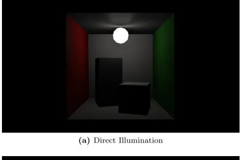
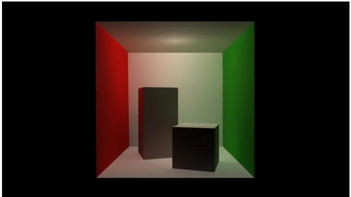
The hybrid rendering system that was developed during this research calcu-lates direct illumination and indirect diffuse illumination separately. In order to compute the radiance at a given point due to direct illumination, we only need to consider the material parameters of its surface and the properties of the light sources that illuminate it (if shadows are taken into account, things become more complicated; our research ignores direct shadows). In contrast, if we want to compute the radiance at a point due to indirect illumination, we need to consider the entire scene (or at least large parts of it) so that we can account for light bouncing around and interacting with multiple surfaces. It is because of this difference that the computation of direct illumination is much less costly than that of indirect illumination. Figure 5.1 shows direct (diffuse and specular) and indirect (diffuse) illumination visualised separately, as well as a final composited render in which both can be observed.

(20)

(a)Direct Illumination

(b)Indirect Diffuse Illumination

[image:20.612.182.430.131.295.2]

(c)Composite Image

(21)

each light pass. It does so by rendering the scene geometry once; but instead of directly rendering it to a shaded output image, it renders certain information to a special purpose buffer so that it can be accessed in later screen-space lighting passes. This buffer is called a geometry-buffer (often abbreviated as G-Buffer) and typically consists of multiple textures. The contents of the G-Buffer, as well as its layout, varies between applications and lighting models.

Deferred shading allows us to render simple bounding geometry for light sources (the intent here is to have the geometry bound the surfaces to be shaded,not

just the light source), which means that the scene geometry does not have to be re-rasterised for each light pass. It is of particular importance to our applica-tion that having a G-Buffer also allows us to easily fetch geometry and material properties of surfaces during the final shading step of our photon mapping im-plementation.

Our system’s rendering process can be outlined as follows:

1. Render the scene accounting only for direct illumination

(a) Render scene geometry to G-Buffer

(b) Scatter light geometry for each light source and accumulate shading results in an output texture

2. Fill photon map with indirect photons

(a) Start photon paths from light sources

(b) Trace paths throughout the scene. Create photons at the closest intersections and store them in the photon map (exclude the first bounce, since we are only interested in indirect illumination during this stage)

3. Assign photons from the photon map to 2D screen-space tiles based on their position

4. Compute indirect illumination for each pixel in the output image by sam-pling nearby photons from the tile in which the pixel is located

5. Composite direct and indirect illumination into a final image

(22)

5.2 Direct Illumination

As mentioned in the previous section, deferred rendering is used to compute the direct lighting in the scene. In this section, we provide a slightly more detailed description of how our deferred renderer implementation is designed.

In order to be able to compute shading due to direct illumination, our deferred renderer first starts a geometry pass. In this pass, information that is required to perform shading is written to the geometry buffer. In subsequent per-light passes, fragment threads are only invoked for pixels that are affected by their respective light source. These threads can access the geometry properties for that given pixel from the G-Buffer.

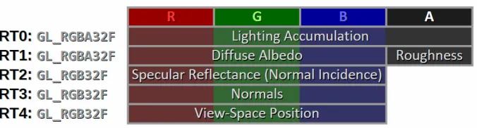
The goal of the geometry pass is to store any information needed to shade a given pixel in the G-Buffer. The contents of the G-Buffer will vary between applications. The layout that is used in our system is visualised in figure 5.2. Storing this information is similar to how conventional forward rendering is done, with the exception that instead of the shader program performing shading calculations and writing to a single output buffer, it directly writes the relevant information to the different render targets of the G-Buffer.

[image:22.612.138.476.479.570.2]

In order to perform shading, the rendering system performs two passes per light source: a stencil pass, and a light pass. The interplay between stencil and light passes ensure that fragment threads are only invoked for fragments that are subtended by geometry within the bounding volume of the light source. The actual shading is performed in the light passes, which write their results into the accumulation part of the G-Buffer (additive blending is used during the light passes for cases where a surface is lit by multiple light sources).

(23)

1 // Derive l from representative point

2 vec3 R=normalize(reflect(-V, N));

3

4 vec3 centerToR =dot(L, R)*R- L;

5 vec3 representativePoint=L+centerToR *

6 clamp(LightRadius /length(centerToR), 0.0f,1.0f);

7

8 vec3 l=normalize(representativePoint);

Listing 5.1: Representative Point Method

1 float a=roughness*roughness;

2 float aa=clamp(a +LightRadius /(2 *distance), 0.0f, 1.0f);

3 float sphereNormalization=pow(a/aa,2);

Listing 5.2: Representative Point Normalisation

5.2.1 Area Lights

In order to achieve real-time area lighting for direct illumination, we have adopted the representative point method proposed by Karis [15]. Although this approach could be used for multiple types of area lights (i.e. spheres, disks and rectangles), our system only supports sphere lights. The main idea behind the representative point method is that the contribution of an area light is ap-proximated by treating all of its emitted light as if it were coming from a single representative point. The result of this approach is that the lighting pipeline hardly differs from conventional point light computation. The only thing that changes is the way in which the direction vector towards the light source is cal-culated, along with an additional normalisation term to ensure that energy is conserved.

So how do we choose this representative point? One way to do this is to choose a point that is likely to have a large contribution to the lighting. A reasonable approximation is to choose a point on the light source that has the smallest angle to the reflection ray. Listing 5.1 shows how this can be computed in GLSL code.

By using this representative point approach, we are effectively widening the specular distribution by the sphere’s subtended angle [15]. If we want to main-tain energy conservation, then the light’s intensity needs to be normalised for this widening. Karis suggests the normalisation term shown in listing 5.2 for the GGX specular BRDF [15].

5.3 Indirect Illumination

(24)

deeper into the individual parts of the process.

The first part of the process is to trace paths throughout the scene and to deposit indirect photons in the photon map. We use the NVIDIA Optix framework [19] to perform ray tracing operations on the GPU. The Optix framework is essentially a flexible ray tracing engine that is built on top of CUDA and as such can be of excellent use to projects that require rapid prototyping of ray tracing applications. However, the flexibility of this framework does come at a cost. Parker et al. have reported seeing a performance penalty of around 30% when comparing Optix to a manually optimized ray tracer [19].

The way in which we compute the radiance estimate is heavily based on the work done by Mara et al. [16]. In their research, a number of different methods for performing the photon density estimation have been compared in terms of quality and performance. We use the method that seemed most promising out of the ones examined, which is a 2D-tiled approach. After the photon tracing stage is complete, the photons in the photon map are assigned to 2D screen tiles. We do this by constructing a frustum for each of the tiles, which allows us to perform intersection test between a photon’s influence sphere and a tile’s frustum. Using this method, we can query for nearby photons in a manner that is easily parrallelisable and translates well to GPUs. Indirect shading is then a matter of iterating over the photons that illuminate a pixel and accumulating their contributions.

Before we delve deeper into how the photon tracing and radiance estimation phases are executed, we will first go over how pseudo random numbers – which are used to sample points on light sources as well as directions in the photon scattering process – are computed on the GPU.

5.3.1 Random Number Generation

Generating samples from a probability density function is something that lies at the basis of all methods that take a Monte Carlo approach. We use the Tiny Encryption Algorithm (TEA) [25] for GPU based random number generation. The study by Zafar et al. shows that the TEA can be used as a random number generator that satisfies all requirements of a good random number generator [26]. In addition, the algorithm allows for a trade off in terms of speed and quality by specifying the number of times it should iterate.

(25)

1 template<optix::uint N>

2 optix::uint2 __device__ TEA(optix::uint v0, optix::uint v1)

3 {

4 optix::uint sum = 0u;

5 for(uint i= 0; i<N; ++i)

6 {

7 sum += 0x9E3779B9;

8 v0 += ((v1 << 4)+ 0xA341316C)^(v1+sum) ^((v1 >> 5)+ 0xC8013EA4);

9 v1 += ((v0 << 4)+ 0xAD90777D)^(v0+sum) ^((v0 >> 5)+ 0x7E95761E);

10 }

11

12 return optix::make_uint2(v0, v1);

13 }

Listing 5.3: CUDA implementation of TEA for pseudo random number generation.

1 optix::float2 __device__ Rnd(optix::uint2&prev)

2 {

3 using namespace optix;

4

5 uint2 newSeed =TEA<8>(prev.x, prev.y);

6 prev =newSeed;

7

8 float2 xi =make_float2(newSeed.x& 0x00FFFFFF, newSeed.y & 0x00FFFFFF);

9 return xi /static_cast<float>(0x01000000);

10 }

Listing 5.4: Random number generator based on TEA.

5.3.2 Photon Tracing

As mentioned before, we use the NVIDIA Optix framework to perform ray tracing on the GPU. The first step to our photon tracing sequence is to emit a number of photons from the light sources in the scene. The photon emission phase is computed in an Optix ray generation program, which serves as an entry point for the Optix ray tracing pipeline.

5.3.2.1 Photon Emission

The photon emission kernel is responsible for initialising a payload data struc-ture that is used throughout the path that a ray follows. This payload is acces-sible and modifiable in following invocations of ray intersection programs. In our case, this data structure is composed of radiant power, a seed for random number generation, and the depth of the current ray in its path (see listing 5.5). Initialising this structure is the first action that is performed by the photon emission program. The radiant power is initialised with the light source’s in-tensity divided by a factor of the number of paths that will be generated. The seed value is initialised by calling theTEAfunction (shown in listing 5.3) with the current kernel invocation’s launch index as its seed. Finally, the depth value is set to zero.

(26)

1 struct RPMH_ALIGN(32) PhotonTracingPRD

2 {

3 optix::float4 power;

4 optix::uint2 seed;

5 optix::uint depth;

6 optix::uint padding;

7 };

Listing 5.5: Definition of the payload structure used during the ray tracing process.

origin for the first ray in its path. Since we are dealing with spherical area lights, we need to be able to generate points on the surface of a sphere. In addition, these points should ideally be spaced out uniformly over the surface of the sphere. The Halton and Hammersley sequences are both low discrepancy sequences that can be used in situations like this [20]. We have opted for the Hammersley sequence since we always know how many samples need to be generated. The two-dimensional Hammersley sequence is based on the simpler one-dimensional van der Corput sequence, which is in turn given by the radical inverse function in base 2. This radical inverse function can be thought of as mirroring the binary representation of its input around the decimal point. The floating point implementation of the radical inverse function, along with example tables and images to make it clearer how this function works can be found in the book by Pharr and Humphreys [20]. See listing 5.6 for an implementation of the radical inverse function in base 2 that uses bitwise operators.

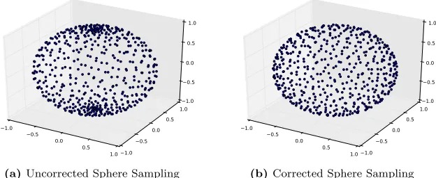
Now that we have described how the low discrepancy number sequences are computed, we can move on to how they are used to sample points on the surface of a sphere light. Since the numbers computed from the Hammersley sequence are two-dimensional, it seems natural to interpret these as spherical coordinates. However, doing so will cause the points to clump up near the poles of the sphere and not have a uniform distribution (this is visualised in figure 5.3a). Instead,

1 float __device__RadicalInverseUint32(optix::uint bits)

2 {

3 bits =(bits << 16u)|(bits>> 16u);

4 bits =((bits & 0x55555555u)<< 1u)|((bits & 0xAAAAAAAAu)>> 1u);

5 bits =((bits & 0x33333333u)<< 2u)|((bits & 0xCCCCCCCCu)>> 2u);

6 bits =((bits & 0x0F0F0F0Fu)<< 4u)|((bits & 0xF0F0F0F0u)>> 4u);

7 bits =((bits & 0x00FF00FFu)<< 8u)|((bits & 0xFF00FF00u)>> 8u);

8 return ((bits >> 8)& 0xFFFFFF)/float(1 << 24);

9 }

10

11 optix::float2 __device__ Hammersley(optix::uint i, optix::uint N)

12 {

13 return optix::make_float2(float(i)/float(N), RadicalInverseUint32(i));

14 }

(27)

−1.0 −0.5 0.0 0.5 1.0 −1.0 −0.5 0.0 0.5 1.0 −1.0 −0.5 0.0 0.5 1.0

(a)Uncorrected Sphere Sampling

−1.0 −0.5 0.0 0.5 1.0 −1.0 −0.5 0.0 0.5 1.0 −1.0 −0.5 0.0 0.5 1.0

[image:27.612.154.466.147.275.2]

(b)Corrected Sphere Sampling

Figure 5.3: Images showing the difference in direct interpretation of samples as spherical coordinates (left) and the application of the correction defined in equation 5.1 (right).

we use the following correction

θ= 2πξ1

φ= cos−1(2ξ2−1),

(5.1)

which gives spherical coordinates representing points that do have a uniform distribution over the unit sphere (shown in figure 5.3b)[24]. We then use the following, which yields the Cartesian coordinates of points on the unit sphere.

u= cosφ

x=√1−u2_cos_θ

y=√1−u2_sin_θ

z=u

(5.2)

Since not all spherical light sources have the same dimensions as the unit sphere, we scale the Cartesian coordinates with the light source’s radius. Adding the light source position to the scaled sample results in the origin of the first ray that corresponds to the sample.

(28)

hemisphere [20]. Computing points uniformly on the unit disk can be done as such:

r=√ξ1

θ= 2πξ2.

(5.3)

These coordinates can then be converted to Cartesian coordinates and be pro-jected onto the unit hemisphere by computing

x=rcosθ y=rsinθ z=√1−ξ1.

(5.4)

Once the payload structure has been initialised and the ray’s origin and direction vectors have been computed, we are ready to continue this ray’s tracing process by invoking thertTrace function. The entire photon emission kernel is shown in listing 5.7.

1 #include <optix_world.h>

2

3 #include "PhotonTracingTypes.h"

4 #include "sampling_utils.h"

5

7

8 rtDeclareVariable(uint, launchIndex, rtLaunchIndex, );

9 rtDeclareVariable(rtObject, topObject, , );

10

11 rtDeclareVariable(float, sceneEpsilon, , );

12 rtDeclareVariable(uint, numPaths, , );

13

14 rtDeclareVariable(float3, lightPosition, , );

15 rtDeclareVariable(float3, lightIntensity, , );

16 rtDeclareVariable(float, lightRadius, , );

17 18

19 RT_PROGRAMvoid PhotonEmission()

20 {

21 PhotonTracingPRD prd;

22 prd.power =make_float4(lightIntensity /float(0.01f * numPaths),1.0f);

23 prd.seed =TEA<16>(launchIndex, launchIndex* 1664525u);

24 prd.depth = 0;

25

26 float2 xi =Hammersley(launchIndex, numPaths);

27 float3 sphereSample= lightRadius*UniformSampleUnitSphere(xi);

28 float3 rayOrigin =lightPosition +sphereSample;

29 float3 rayDirection= CosineSampleHemisphere(normalize(sphereSample), Rnd(prd.seed));

30

31 Ray ray =make_Ray(rayOrigin, rayDirection, 0, sceneEpsilon, RT_DEFAULT_MAX);

32 rtTrace(topObject, ray, prd);

33 }

(29)

5.3.2.2 Photon Scattering

Optix supports three different types of programs that can be invoked based on how the ray intersects the scene. These are the closest hit, any hit, and miss programs. In order to implement photon scattering, we do not need the any hit or miss programs and as such only register a closest hit program that contains our photon scatting behaviour. This is thus a program that is invoked whenever the ray tracing system has found the closest surface with which the ray intersects.

Since we want photons to describe light that is incident on a surface, they need to be created and deposited in the photon map before they reflect off of the surface. At this stage, the photon map is simply an array of structures that describe the photon’s position, incoming power, and incident direction (see definition of

OptixPhotonin listing 5.8). In order to keep the size of this photon structure

at 32 bytes, we’ve chosen to encode the direction vector into two float values here, and later decode the direction vector when the photon structures need to be read. The encoding/decoding scheme we use is the Octahedral Normal Vector (ONV) method as described by Meyer et al. and Cigolle et al. [18][3] (it is called oct instead of ONV in the work by Cigolle et al.). We show the implementation of the encoding function in listing 5.9 (the decoding function is shown in listing 5.16 on page 35).

Since we are dealing with a large number of threads running in parallel, we need a system in place that guarantees each thread is able to safely deposit photons into the photon buffer. To achieve this we use a shared counter that is atomically incremented whenever a thread wishes to deposit a photon. This

1 struct RPMH_ALIGN(32) OptixPhoton

2 {

3 optix::float3 position;

4 optix::float3 power;

5 optix::float2 direction;

6 };

Listing 5.8: Definition of photon during the photon tracing process.

1 float2 __device__ SignNotZero(constfloat2&v)

2 {

3 return make_float2((v.x >= 0.0f)? +1.0f : -1.0f, (v.y >= 0.0f)? +1.0f : -1.0f);

4 }

5

6 float2 __device__ ONVEncode(constfloat3& v)

7 {

8 float2 p =make_float2(v) *(1.0f / (abs(v.x) +abs(v.y) +abs(v.z)));

9 return (v.z <= 0.0f)?((1.0f - make_float2(abs(p.y), abs(p.x))) *SignNotZero(p)) :p;

10 }

(30)

counter’s old value is then used as an index for the photon buffer. When a photon has been deposited in the photon buffer – and the maximum path depth has not yet been reached – the kernel generates new random numbers, selects an outgoing direction using importance sampling, attenuates the photon power and finally updates the payload structure. After this, the ray tracing process can continue along its path, possibly resulting in additional program invocations and eventually resulting in the photon buffer being filled with indirect photons. The entirety of the photon scattering program is shown in listing 5.10.

5.3.3 Radiance Estimate

The objective of the radiance estimate step is to approximate the outgoing radiance that is directed towards the camera from a given surface. The method applied in this research is a 2D-tiled approach based on the work of Mara et al. [16]. We summarise the process here briefly and provide more details in the following sections.

The screen is first divided into a number of two dimensional tiles whose bounds are used to construct frustra. These frustra are in turn used to assign photons to certain tiles based on whether the photons and tile frustra intersect. During the indirect shading of a given pixel, nearby photons can be sampled by iterating over the photons that are stored in the tile encompassing that pixel. Using the set of nearby photons, we can approximate the indirect diffuse component of the reflectance equation (shown in equation 2.6 on page 8). This process will be described in more detail later on; first, we delve into how photons are assigned to the specific tiles.

5.3.3.1 Photon Counting and Tile Insertion

For this part of the algorithm, the objective is to create a data structure that allows us to sample photons that are spatially near to (areas of) surfaces in the scene that are represented by pixels in the G-Buffer. The use case is that while a given pixel is being shaded, we want to be able to iterate over a relatively small subset of nearby photons. The research by Mara et al. [16] compares several methods that do this in real-time, both in terms of visual quality and performance. Based on the results of their research, we have chosen to adopt a tiled approach. This method divides the viewport into a number of 2D-tiles. The bounds of these tiles are used to create frustra that are used to assign photons to the corresponding tile based on whether their influence sphere intersects the tile’s frustum.

(31)

1 #include <optix_world.h>

2

3 #include "PhotonTracingTypes.h"

4 #include "sampling_utils.h"

5

7

8 rtBuffer<OptixPhoton> outputBuffer;

9 rtBuffer<uint> photonCountBuffer;

10

11 rtDeclareVariable(rtObject, topObject, , );

12 rtDeclareVariable(float, sceneEpsilon, , );

13 rtDeclareVariable(uint, maxPathDepth, , );

14 rtDeclareVariable(uint, maxNumPhotons, , );

15

16 rtDeclareVariable(float3, Kd, , );

17 rtDeclareVariable(float, lambertianProbability, , );

18

19 rtDeclareVariable(Ray, ray, rtCurrentRay, );

20 rtDeclareVariable(float, t_hit, rtIntersectionDistance, );

21 rtDeclareVariable(PhotonTracingPRD, prd, rtPayload, );

22

23 rtDeclareVariable(float3, shadingNormal, attribute shadingNormal, );

24 rtDeclareVariable(float3, geometricNormal, attribute geometricNormal, );

25

26 RT_PROGRAMvoid ClosestHit()

27 {

28 float3 hitPosition =ray.origin+t_hit *ray.direction;

29

30 // We are only interested in storing indirect photons

31 if(prd.depth > 0)

32 {

33 uint photonIndex =atomicAdd(&photonCountBuffer[0],1);

34

35 // Break if output buffer is full

36 if(photonIndex>=maxNumPhotons) return;

37

38 // Deposit photon into output buffer

39 OptixPhoton photon;

40 photon.position =hitPosition;

41 photon.power =make_float3(prd.power);

42 photon.direction =ONVEncode(ray.direction);

43 outputBuffer[photonIndex] =photon;

44

45 // Break if maximum path depth has been reached

46 if(prd.depth>=maxPathDepth) return;

47 }

48

49 float3 omega_i =ray.direction;

50 float3 shadingNormalWS =

51 normalize(rtTransformNormal(RT_OBJECT_TO_WORLD, shadingNormal));

52 float3 geometricNormalWS =

53 normalize(rtTransformNormal(RT_OBJECT_TO_WORLD, geometricNormal));

54 float3 N =faceforward(shadingNormalWS, -omega_i, geometricNormalWS);

55

56 float2 xi =Rnd(prd.seed);

57 float3 omega_o =CosineSampleHemisphere(N, xi);

58 float3 color =make_float3(prd.power)* Kd/M_PIf /lambertianProbability;

59 prd.power =make_float4(color, 1.0f);

60

61 prd.depth++;

62

63 Ray newRay= optix::make_Ray(hitPosition, omega_o, 0, sceneEpsilon, RT_DEFAULT_MAX);

64 rtTrace(topObject, newRay, prd);

65 }

(32)

currently copied from GPU memory to main memory and back to GPU memory since we are switching from a CUDA buffer to an OpenGL buffer). The second buffer contains indices to the photons in the photon buffer. The tiled structure is introduced by the third buffer, which we call the tile metadata buffer. This buffer contains elements that each represent a tile and describe where the photon indices that belong to this tile can be found (this is achieved by keeping track of the number of photons that intersect this tile as well as an offset into the photon index buffer). See listing 5.11 for the GLSL declaration of these buffers.

To avoid having to over-allocate the photon index buffer, we have split the tiling process into two phases. These two phases are very similar to one another; they construct frusta based on tile bounds and perform intersection tests between these and the photon’s influence spheres. The first phase, however, only counts the number of photons that intersect a tile’s frustum and stores this information in the tile metadata buffer. After all kernels have completed the photon counting process, we iterate over the elements in the tile metadata buffer on the CPU, setting the index offsets to their correct values by keeping count of the total number of indices in all preceding tiles. At this point the photon index buffer is allocated so that it can be populated during the tile insertion pass.

As mentioned previously, the photon counting and tile insertion kernels are very similar to one another. Thus, we will only go through the implementation of the tile insertion pass. Listing 5.12 partially shows the code that is used as the tile insertion kernel. Both the photon counting and tile insertion passes

1 struct Photon

2 {

3 vec4 position;

4 vec4 power;

5 };

6

7 struct TileMetadata

8 {

9 uint offset;

10 uint numPhotons;

11 };

12

13 layout (binding = 0, std430) buffer photonBuffer

14 {

15 Photon photons[];

16 };

17

18 layout (binding = 1, std430) buffer photonIndexBuffer

19 {

20 uint photonIndices[];

21 };

22

23 layout (binding = 2, std430) buffer tileMetadataBuffer

24 {

25 TileMetadata tileMetadata[];

26 };

(33)

1 #version 430

2 #define USE_HIGH_RES_TILES

3 include(Commons.c.glsl)

4

5 layout (binding = 0)uniform sampler2D depthStencil;

6

7 uniform uvec2 gBufferDimensions;

8 uniform mat4 projectionMatrixInv;

9 uniform mat4 viewMatrix;

10 uniform uint numPhotons;

11

12 shared uint localIndexCounter;

13 shared uint localZMin;

14 shared uint localZMax;

15

16 include(PhotonTilingUtils.c.glsl)

17

18 void main()

19 {

20 uint localIndex =gl_LocalInvocationIndex;

21 uint tileIndex =gl_WorkGroupID.x+gl_WorkGroupID.y *gl_NumWorkGroups.x;

22

23 // Initialize shared variables

24 if(localIndex == 0)

25 {

26 localIndexCounter = 0;

27 localZMin = 0xffffffff;

28 localZMax = 0;

29 } 30 31 barrier(); 32 ComputeLocalDepthBounds(); 33 34 barrier();

35 float zMin= uintBitsToFloat(localZMin);

36 float zMax= uintBitsToFloat(localZMax);

37 uint offset =tileMetadata[tileIndex].offset;

38

39 vec4 frustumEqn[4];

40 CreateTileFrustumEqn(frustumEqn);

41 for(uint i= localIndex; i<numPhotons; i += NUM_THREADS_PER_TILE)

42 {

43 Photon photon =photons[i];

44 vec4 photonPos =viewMatrix*vec4(photon.position.xyz, 1.0f);

45

46 if(photonPos.z+zMin <photonInfluenceRadius&&

47 -photonPos.z -zMax <photonInfluenceRadius)

48 {

49 if((SignedDistanceFromPlane(photonPos, frustumEqn[0]) <photonInfluenceRadius) &&

50 (SignedDistanceFromPlane(photonPos, frustumEqn[1]) <photonInfluenceRadius) &&

51 (SignedDistanceFromPlane(photonPos, frustumEqn[2]) <photonInfluenceRadius) &&

52 (SignedDistanceFromPlane(photonPos, frustumEqn[3]) <photonInfluenceRadius))

53 {

54 uint idx =atomicAdd(localIndexCounter,1);

55 photonIndices[offset+idx] =i;

56 }

57 }

58 }

59 }

(34)

are started by calling glDispatchCompute with the number of tiles in the x and y directions as the number of work groups in the respective directions.

We use a tile size of 8×8, which means that each work group consists of

64 threads. Threads within a work group can communicate with each other through shared variables, which for the most part behave as global variables for all kernel invocation within the same work group. However, we do have to manually initialise these shared variables and synchronise the threads so that shared variable visibility is ensured. We synchronise the threads and ensure shared variable visibility by calling thebarrier()function at certain locations (see lines 31 and 34). This function forces synchronisation between all kernel invocations in the work group, meaning that execution within the work group will not proceed until all other invocations have reached the barrier. Once the barrier function exits, all shared variables will be visible to the other invocations of the work group. The shared variables themselves are declared at lines 12 to 14 and are initialised by a single designated kernel invocation within the work group at lines 24 to 29.

Before we construct the frustra we first determine the minimum and maximum depth value that is present in the G-Buffer within the bounds of the tile. Each kernel invocation can correspond to a single pixel from the G-Buffer. This means that all we have to do is read the depth value for the given thread from the G-Buffer and perform atomic minimum and maximum operations on the shared variables that keep track of the lowest and highest depth values. This is done

in theComputeLocalDepthBounds() function, of which the implementation is

shown in listing 5.13. Note that the localZMinand localZMaxvariables are

unsigned integers despite our depth values being stored as floats. This is due to the fact that the atomic operations that can be used on shared variables

only support signed and unsigned integers. Thus, we reinterpret the depth

value as an unsigned integer before applying the atomic operations (see line 8 in listing 5.13) and again reinterpret the unsigned integer as a float after we have found the minimum and maximum values (see lines 35-36 in listing 5.12). The

uintBitsToFloatand floatBitsToUintfunctions preserve the floating-point

bit-level representation.

1 void ComputeLocalDepthBounds()

2 {

3 vec2 texCoord =vec2(gl_GlobalInvocationID.xy + 0.5f)/ vec2(gBufferDimensions);

4 float z=texture(depthStencil, texCoord).r;

5

6 if(z != 0.0f)

7 {

8 uint linearZ =floatBitsToUint(LinearizeDepth(z));

9 atomicMin(localZMin, linearZ);

10 atomicMax(localZMax, linearZ);

11 }

12 }

(35)

The final part of the tile insertion kernel is to construct frustra based on the tile bounds, and to perform intersection tests between them and the photon influence spheres. Each kernel invocation creates plane equations for the four sides of the frustum by calling theCreateTileFrustumEqn()function (see list-ing 5.14 for the implementation details). The construction of the frustum plane equations, as well as the methods we use for photon-tile intersection tests, are based on the light culling methods shown in the work by Harada et al. in [9] (at the time of writing AMD has also published code samples that show additional examples of how this can be done).

We divide the photons over the kernel invocations by using a for-loop that starts

1 vec4 CreatePlaneEquation(vec4v1, vec4v2)

2 {

3 return vec4(normalize(cross(v1.xyz, v2.xyz)), 0.0f);

4 }

5

6 floatSignedDistanceFromPlane(vec4 p, vec4 planeEqn)

7 {

8 return dot(planeEqn.xyz, p.xyz);

9 }

10

11 void CreateTileFrustumEqn(out vec4 frustumEqn[4])

12 {

13 uvec2 correctedWindowDimensions =gl_WorkGroupSize.xy*gl_NumWorkGroups.xy;

14 vec2 corrDim=vec2(correctedWindowDimensions);

15

16 uvec2 pMin=gl_WorkGroupSize.xy*gl_WorkGroupID.xy;

17 uvec2 pMax=gl_WorkGroupSize.xy*(gl_WorkGroupID.xy + 1);

18

19 vec4 frustum[4];

20 frustum[0]=ProjectionToView(vec4(

21 pMin.x /corrDim.x * 2.0f- 1.0f,

22 pMin.y /corrDim.y * 2.0f- 1.0f,

23 1.0f, 1.0f));

24

26 pMax.x /corrDim.x * 2.0f- 1.0f,

27 pMin.y /corrDim.y * 2.0f- 1.0f,

28 1.0f, 1.0f));

29

31 pMax.x /corrDim.x * 2.0f- 1.0f,

32 pMax.y /corrDim.y * 2.0f- 1.0f,

33 1.0f, 1.0f));

34

36 pMin.x /corrDim.x * 2.0f- 1.0f,

37 pMax.y /corrDim.y * 2.0f- 1.0f,

38 1.0f, 1.0f));

39

40 for(uint i= 0; i< 4;++i)

41 {

42 frustumEqn[i] =CreatePlaneEquation(frustum[i], frustum[(i + 1)% 4]);

43 }

44 }

(36)

on the local thread index (this is the index of a thread within the work group) and is incremented by the number of threads per tile (see line 41 in listing 5.12). Each photon’s position is then transformed into view space and a series of tests are performed to determine if the photon’s influence sphere intersects the frustum (lines 43-57 in listing 5.12). If a photon’s influence sphere is found

to be intersecting the frustum, we increment the shared localIndexCounter

variable and insert the photon’s index into the photon index buffer (lines 54-55 in listing 5.12).

After the photon counting and tile insertion passes have finished executing, the photon map (which now consists of the photon buffer, the photon index buffer and the tile metadata buffer) will be filled with the necessary information needed to perform the indirect shading pass.

5.3.3.2 Shading Indirect Illumination

Computing the outgoing radiance at a visible surface in the scene is now rela-tively straightforward. For a given pixel we can now determine what the corre-sponding tile is, sample the nearby photons by iterating over the relevant parts of the photon map, and finally perform shading for the given pixel. Seeing as the number of photons that will be used will generally be relatively low, it is important that the radiance estimate is filtered so that edges of the photon influence spheres do not become discernible. There are of course multiple ways in which this can be done, but we have chosen to use a simple cone filter as described by Jensen [11]. This filter assigns a weight,wp, to photons based on

the distance between the photon and the surface area that is being shaded. The photon weights are computed as

wp= 1−

dp

kr, (5.5)

wheredpis the distance between the photon and the surface area being shaded,

kis a filter constant that characterises the filter, andris the maximum distance allowed between the photon and the surface area. The normalisation term for this filter is 1− 2

3k, which means that the radiance can be approximated by

computing

Lr(x,wo)≈

∑N

p=0fr(x,wi,wo)Φp(x,wi)wp

(1− 2 3k)πr2

. (5.6)

(37)

1 vec3 RadianceEstimate(uint tileIndex,vec3 albedo, vec3N, vec3 positionVS)

2 {

3 TileMetadata tile =tileMetadata[tileIndex];

4 uint indexOffset =tile.offset;

5 uint numPhotonsInTile =tile.numPhotons;

6

7 vec3 accumulation=vec3(0.0f);

8 for(unsigned inti= 0; i<numPhotonsInTile; ++i)

9 {

10 Photon photon =photons[photonIndices[indexOffset +i]];

11 vec3 photonPosition =photon.position.xyz;

12 vec3 photonPower =photon.power.xyz;

13 vec3 photonDirection =ONVDecode(vec2(photon.position.w, photon.power.w));

14

15 vec3 photonPositionVS =(viewMatrix* vec4(photonPosition,1.0f)).xyz;

16 float dist =distance(photonPositionVS, positionVS);

17 if(dist>photonInfluenceRadius) continue;

18

19 vec3 L= -normalize(rotationMatrix *photonDirection);

20 float NdotL=clamp(dot(N, L), 0.0f, 1.0f);

21 float photonWeight= 1 -(dist /photonInfluenceRadius);

22 accumulation +=photonPower *photonWeight* albedo/ PI*NdotL;

23 }

24

25 accumulation /=(1.f- 2.f/ 3.f)*PI *photonInfluenceRadius* photonInfluenceRadius;

26 return accumulation;

27 }

Listing 5.15: GLSL implementation of the radiance estimation function.

1 vec2 SignNotZero(vec2v)

2 {

3 return vec2((v.x >= 0.0f) ? +1.0f: -1.0f, (v.y>= 0.0f) ? +1.0f : -1.0f);

4 }

5

6 vec3 ONVDecode(vec2e)

7 {

8 vec3 v=vec3(e.xy,1.0f-abs(e.x) -abs(e.y));

9 if(v.z < 0.0f) v.xy= (1.0f-abs(v.yx))*SignNotZero(v.xy);

10 return normalize(v);

11 }

Listing 5.16: GLSL implementation of functions that decode two floats to avec3

using the ONV method.

Additionally, we show the implementation of theONVDecodefunction in listing 5.16. This function decodes two float values to a three-component float vector. To see how the photon direction is encoded see listing 5.9 on page 27.

5.3.4 Further Approximations

(38)

during the final pass that combines the direct and indirect illumination. Using linear interpolation will for the most part provide good results that are nearly identical to the radiance estimate at full resolution. However, the results will deviate greatly around geometry edges which will in turn appear blurry. To combat this, we use a simple edge detection scheme and recompute the radiance estimate around these edges. This edge detection scheme is based on finding differences in normals and positions of visible surface areas. To do this we write these normals and positions to low resolution textures in addition to the estimated radiance. During the final pass that combines direct and indirect illumination, we sample the normals and positions from both the low resolution textures and the G-Buffer (full resolution). The normals are compared using a dot product, whereas the positions are checked using a distance function. If the normals and positions are similar enough, we sample the indirect illumination from the low resolution texture using linear interpolation. If either the normals or positions differ too much we recompute the radiance estimate.

We show the implementation of the pass that renders to a low resolution texture array in listing 5.17. The implementation is relatively simple; we read the necessary information from the G-Buffer (lines 26-28), perform the radiance estimate using the function that was shown in listing 5.15 (line 30), and finally store the estimated radiance, normal and position in the low resolution texture array (lines 32-34).

The final pass is shown in listing 5.18. This kernel reads the normals and

positions from both the G-Buffer and the low resolution texture array (lines 28-31), evaluates whether the precomputed radiance estimate can be used (lines 33 and 36) and responds accordingly (lines 38-39, and line 43). After the indirect illumination has been computed, we read the direct illumination from the G-Buffer, combine it with the indirect illumination and finally write the output back to the light accumulation part of the G-Buffer, which will be displayed at the end of the frame.

(39)

1 #version 430

2

4

5 layout (binding = 2)uniform sampler2D RT1; // Kd + Ns

6 layout (binding = 3)uniform sampler2D RT2; // Ks + Ni

7 layout (binding = 4)uniform sampler2D RT3; // Normals

8 layout (binding = 5)uniform sampler2D RT4; // Position

9

10 layout (binding = 6)uniformwriteonly image2DArray LowResTextureArray;

11

13 uniform mat3 rotationMatrix;

14 uniform uvec2 indirectTextureDimensions;

15

16 const float PI = 3.14159265f;

17

18 include(RadianceEstimate.c.glsl)

19

20 void main()

21 {

23 ivec2 imageCoord=ivec2(gl_GlobalInvocationID.xy);

24 vec2 texCoord =vec2(imageCoord + 0.5f) /vec2(indirectTextureDimensions);

25

26 vec3 albedo =texture(RT1, texCoord).rgb;

27 vec3 N=texture(RT3, texCoord).xyz;

28 vec3 positionVS=texture(RT4, texCoord).xyz;

29

30 vec3 indirectLighting =RadianceEstimate(tileIndex, albedo, N, positionVS);

31

32 imageStore(LowResTextureArray, ivec3(imageCoord, 0), vec4(indirectLighting, 1.0f));

33 imageStore(LowResTextureArray, ivec3(imageCoord, 1), vec4(N,1.0f));

34 imageStore(LowResTextureArray, ivec3(imageCoord, 2), vec4(positionVS,1.0f));

35 }

(40)

1 #version 430

2

3 #define USE_HIGH_RES_TILES

5

6 layout (binding = 1, rgba32f)uniformimage2D RT0;

7

8 layout (binding = 2)uniform sampler2D RT1; // Kd + Ns

9 layout (binding = 3)uniform sampler2D RT2; // Ks + Ni

10 layout (binding = 4)uniform sampler2D RT3; // Normals

11 layout (binding = 5)uniform sampler2D RT4; // Position

12 layout (binding = 6)uniformsampler2DArray LowResTextureArray;

13

15 uniform mat3 rotationMatrix;

16 uniform uvec2 gBufferDimensions;

17

18 const float PI = 3.14159265f;

19

20 include(RadianceEstimate.c.glsl)

21

22 void main()

23 {

25 ivec2 imageCoord=ivec2(gl_GlobalInvocationID.xy);

26 vec2 texCoord =vec2(imageCoord + 0.5f) /vec2(gBufferDimensions);

27

28 vec3 N=texture(RT3, texCoord).xyz;

29 vec3 positionVS=texture(RT4, texCoord).xyz;

30 vec3 lowResNormal=texture(LowResTextureArray, vec3(texCoord,1)).xyz;

31 vec3 lowResPositionVS =texture(LowResTextureArray,vec3(texCoord,2)).xyz;

32

33 float positionDiff=distance(positionVS, lowResPositionVS);

34

35 vec4 indirect =vec4(0.0f,0.0f, 0.0f, 1.0f);

36 if(dot(N, lowResNormal) < 0.99f|| positionDiff> 0.01f)

37 {

38 vec3 albedo =texture(RT1, texCoord).rgb;

39 indirect.xyz =RadianceEstimate(tileIndex, albedo, N, positionVS);

40 }

41 else

42 {

43 indirect = texture(LowResTextureArray,vec3(texCoord, 0));

44 }

45

46 vec4 direct =imageLoad(RT0, imageCoord);

47 imageStore(RT0, imageCoord, direct +indirect);

48 }

(41)

Chapter 6

Evaluation

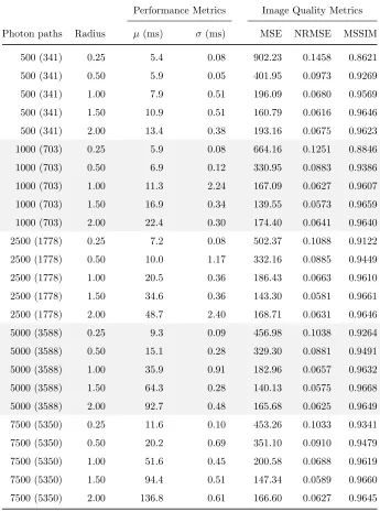
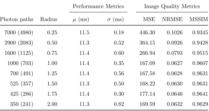
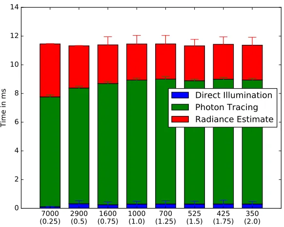
The evaluation of our prototype system is performed in three parts. During this evaluation, we use a number of objective measures to assess the performance of our system in terms of visual quality and computational speed (these metrics have already been discussed in chapter 4). The first two parts of the evaluation focus on our system in isolation. First, we measure how our system performs during the rendering of a simple scene while certain system parameters are varied. Thereafter, we test how computational costs change as scene complexity is varied. In the third and final part, we perform a brief comparative study between our prototype implementation and other systems currently available in game engines.

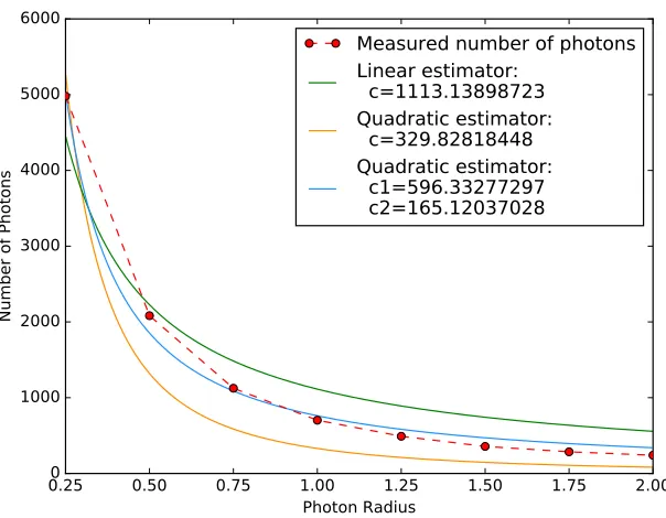
6.1 Parameter Scaling

The rendering parameters that are most impactful on the performance of our system are the total number of photons, and the photon influence radius. The number of photons that are stored in the photon map are indirectly specified via the total number of photon paths that are initiated. We make this distinction because, if a photon path never intersects any scene geometry, it will not result in any stored photons. Since we only compute single-bounce indirect illumination, the number of stored photons will always be lower than the number of initiated photon paths. Whenever we report the number of photon paths, we also report the actual number of stored photons in brackets for completeness.

GPU Based Photon Mapping for Approximate Real Time Indirect Diffuse Illumination

Master Thesis