An agent based compositional framework for supply chain simulation

A Thesis Submitted for the Degree of PhD at the University of Warwick

http://go.warwick.ac.uk/wrap/36393

This thesis is made available online and is protected by original copyright. Please scroll down to view the document itself.

Framework for Supply Chain Simulation

Raghu Arunachalam

Submitted for the degree of Doctor of Philosophy

VERs

-WAJQICK

University of Warwick Department of Engineering

LIST OF FIGURES . 1

LISTOF TABLES ...ii

ACKNOWLEDGMENTS ...iii

DECLARATION ...iv

ABSTRACT ... V ABBREVIATIONS ...vi

1. INTRODUCTION ...1

1.1 Objectives ...6

1.2 Methodology ...6

1.3 Chapter plan ...7

2. A REVIEW OF DISCRETE EVENT SIMULATION AND SUPPLY CHAINMODELLING ...9

2.1 The need for models...9

2.2 World views ...12

2.2.1 Event based approaches...12

2.2.2 Activity based approaches...14

2.4 Overview of developments in discrete event simulation ...21

2.4.1 Programming approaches...21

2.4.2 Non programming approaches...23

2.5 Supply chain modelling ... 25

2.6 Supply chain dynamics ...32

2.7 The role of DES in supply chain modelling ... 35

2.8 Requirements for DES of supply chains ...39

2.9 Web based and distributed modelling ...43

2.10 Conclusion ...46

3. LARGE SCALE MODELLING - A REVIEW ...48

3.1 Modularity and the world views ... 50

3.2 Object oriented simulation ...60

3.3 DEVS and hierarchical modelling ...62

3.3.1 Large scale modelling decomposition and synthesis... 65

3.3.2 Variable structure modelling and DEVS...67

3.4 Coupling schemes ...71

3.5 High level architecture ...73

4.1 The problem ...78

4 .1.1 The structure of asynchronous PDES...79

4 .1.2 Causality errors...80

4.2 PDES algorithms ...82

4.2.1 Conservative approach...82

4.2.1.1 The Chandi and Misraapproach...82

4.2.1.2 Synchronous approach and conservative time windows...86

4.2.2 Optimistic approach...88

4.2.2.1 Rollback control and antimessages...89

4.2.2.2 Global virtual time...91

4.2.2.3 Variations of time warp...93

4.3 Conservative versus optimistic techniques - a critique ...94

4.4 PDES based simulation languages ...96

4.5 PDES of manufacturing systems - a review ...97

4.6 Conclusion ...101

5. A FRAMEWORK FOR COMPOSITE MODELLING ...103

5.1 Design rationale ...103

5.2 Functional view of the architecture ...110

5.3 Composite modelling framework - Process view ...114

5.3.1 Model Taxonomy...114

5.3.2 Model selection...118

5.3.3 Agents and model synthesis...120

5.3.4 Composite model building...124

5.3.5 Simulation of the composite model...132

5.3.5.1 Model encapsulation and model_agents... 133

5.3.5.2 Distributed computer infrastructure...135

5.3.5.3 Simulation super executive...136

5.3.5.4 Local simulation executive...138

5.3.5.5 PDES controller...139

5.4 Conclusion ...140

6. PDES CONTROLLER FOR HERMIS ...141

6.1 The conservative approach ...143

6.2 Optimistic approach ...147

6.3 PDES paradigm ...150

6.3.1 Modified LP architecture...152

6.3.2 PDES algorithm...153

7. CONCLUSION ...170

7.1 Summary of work ...170

7.2 Conclusions ...173

7.3 Contribution ...175

7.4 Suggestions for future work...176

REFERENCES ...178

APPENDICES ...191

Figure 2.1 Forms of supply chain network [Scwarz 811...26

Figure 2.2 Demand amplification in a supply chain [Hulian 87]...32

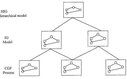
Figure 3.1 Relationship between CFG, IG and HIG... 54

Figure 3.2 Coupling two models using the Entity-Coimection view... 56

Figure 3.3 An example of a simplified PaInt model [Davis 96]... 57

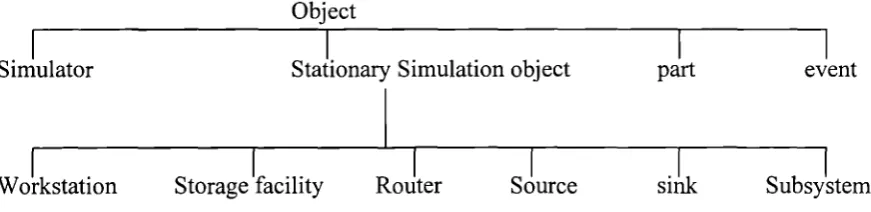
Figure 3.4 ' The class Hierarchy of simulation objects in SmartSim...62

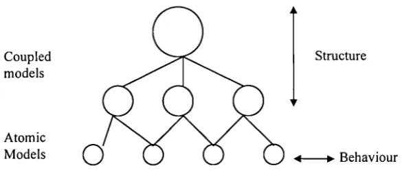
Figure 3.5 Separation of description of behaviour and structure in DEVS models...68

Figure3.6 Simulation of federates in HLA...76

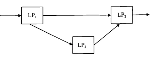
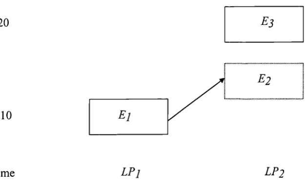
Figure4.1 An example of an LP framework...80

Figure4.2 Causal relationships...81

Figure4.3 An example of deadlock...84

Figure 5.1 Levels of composition (modified from [Davis 96 _1)...104

Figure 5.2 An example of a supply chain of a personal computer manufacturer...108

Figure 5.3 A functional view of the composite modelling framework...110

Figure 5.4 Class hierarchies: a) PC manufacturer, b) Computer monitor Manufacturer...116

Figure 5.5 Transfer-Entity heirarchy of a customer order placed with a PC Manufacturer...118

Figure 5.6 synthesis_agent architecture...122

c. CPU manufacturer...131

Figure 5.10 Architecture of simulation mechanism...135

Figure 6.1 Cyclic relationship in supply chain models... 145

Figure6.2 Modified LP architecture...153

LIST OF TABLES

Table 4.2 Comparison of conservative versus optimistic schemes...96

During the course of my study I have been fortunate to have had the support of many.

Foremost I owe my sincerest gratitude to my supervisor Mr. Rajat Roy for having been a

constant source of guidance and inspiration. I would like to thank the members of the

simulation team for always being helpful and a joy to be amongst.

I am grateful to the Warwick Manufacturing Group and the Department of Engineering

for making my study possible by supporting me financially.

I declare that the work presented in this thesis, unless otherwise acknowledged, is my

own and has not been previously submitted for any academic degree.

To survive in an ever increasing global and competitive marketplace, organisations are forging strategic alliances to gain a competitive advantage over their rivals. Consequently, it is now recognised that it is not sufficient to look at organisations in isolation, but view them in the wider context of the supply chain. In order to design arid manage supply chains it is necessary to understand and predict the behaviour of such systems.

The ability to perform detailed studies of dynamic behaviour has made discrete event simulation (DES) an invaluable tool in the design and analysis of manufacturing systems. DES has been used to model individual stages of a supply chain, but rarely has it been applied comprehensively across the entire chain. The multi-faceted nature of supply chains makes the creation of a single model that represents all aspects of the chain difficult. A compositional framework, termed HerMIS (Heterogeneous Model Integration and Simulation), is proposed that allows pieces of a supply chain to not only be studied in isolation, but in the context of the other parts as well.

Three requirements are identified for the development of HerMIS. These are: (1) to support a compositional approach so as to allow multi-facetted modelling, (2) to function in a distributed environment where models and information about them are distributed at different locations amongst various organisations, and (3) to provide an execution mechanism that allows the composite model to be simulated efficiently.

A class based taxonomy of component models and their interaction is conceived that forms the basis of a representation scheme for composite modelling. An agent based paradigm that employs a collection of synthesis_agents and model_agents is devised to support the distributed operation of the framework. The synthesis_agents function as sources of knowledge for synthesising composite models and are used in conjunction with an interactive blackboard based system to guide the user in creating composite models. Each of the model_agents incorporate a discrete event model of a supply chain component, arid supports the distributed simulation of the composite model.

AS Activity Scanning approach (Discussed in Chapter 2 page 14)

CFG Control Flow Graph ( Discussed in Chapter 3 Page 52)

CCP Component Configuration Packet (Discussed in Chapter 5 Page 137)

DEDM Discrete Event Dynamic Modelling (Discussed in Chapter 2 Page 12)

DES Discrete Event Simulation (Discussed in Chapter 2)

DEVS Discrete Event simulation Specification (Discussed in Chapter 3 Page 62)

ES Event scheduling approach (Discussed in Chapter2 Page 12)

GISS Generalised Interactive based Simulation System (Discussed in Chapter 3

Page 59)

GPPL GUI GVT HerMIS HCFG HIG HLA IG LP MI 00 OOS PAInt PDES

General Purpose Programming Language (Discussed in Chapter 2 Page 21)

Graphical User Interface

Global Virtual Time (Discussed in Chapter 4 Page 91)

Heterogeneous Model integration and Simulation (Discussed in Chapter 5)

Hierarchical Control Flow Graph (Discussed in Chapter 3 Page 52)

Hierarchical Interconnection Graph (Discussed in Chapter 3 Page 52)

High Level Architecture (Discussed in Chapter 3 Page 73)

Interconnection Graph (Discussed in Chapter 3 Page 52)

Logical Process (Discussed in Chapter 4 Page 79)

Model Interaction (Discussed in Chapter 5 Page 114)

Object Oriented

Object Oriented Simulation (Discussed in Chapter 3 Page 60)

Process Activity Interaction (Discussed in Chapter 3 Page 57)

PP Physical Process (Discussed in Chapter 4 Page 79 )

SES System Entity Structure (Discussed in Chapter 3 Page

₆₅₎

CHAPTER 1

Introduction

In an increasingly global and competitive market place, the notion of supply chain and its

management has been the focus of many researchers and practitioners alike. In a fast

changing environment organisations are focusing on their core competencies and forging

strategic alliances that share knowledge and resources to gain a competitive advantage

and retain flexibility over their competitors.

A number of terms such as extended enterprise, virtual enterprises [Bleecker 94] and

symbiotic networks [Alter 93] have been used to describe these integrated enterprises. In

order to get the benefit of such integrated enterprises it is clearly not enough to optimise

one part of the supply chain but to look at it as a whole. In addition to understanding the

components of the system, it is important to understand the relationship between the

various components and the behaviour that consequently emerges.

The developments in network technologies such as the internet and the use of EDT has

enabled the creation of inter-organisational systems that support these emerging close

relationships between organisations. However, the primary focus has been on

implementing transaction systems, such as order, invoice, and payment systems [Turner

a need for integrated decision support systems that help to plan and predict the

performance of the system.

Discrete event simulation (DES) has been used as a tool to analyse the performance of

existing and proposed manufacturing systems for a number of years now. It has been

used to support decision making at various levels from strategic analysis of a proposed

plant to aiding day to day operations, for instance, in a scheduling system. The ability to

create detailed models that closely conform in structure, dynamic and stochastic

behaviour, to the manufacturing system being modelled, has made DES an attractive

technique for what - if analysis. However, DES has largely been restricted to modelling

individual pieces, such as a single production facility of a supply chain and is seldom

employed to model the entire supply chain [Geller 95]. Even in cases where an attempt

has been made to model the supply chain more comprehensively, the modelling effort

can often be described as 'modelling in the small', a term coined by Zeigler [Zeigler 84].

Often a model is created with the purpose of aiding a given decision objective. For

instance, the objective may be to study the potential capacity of a proposed plant. Once

this objective is met the model is viewed as having served its purpose and is often

discarded. Even in the case of a DES model developed in the context of a scheduling

system, where a model is used over a long period of time, it is still generally confined to

this application. If for instance the scheduling problem is to be studied at a supply chain

level instead of at a local level, then typically, a new model is created from scratch rather

to eighty percent of simulation models developed in the automobile industry fall into this

category of 'modelling in the small'.

The nature of supply chain management is such that a multiplicity of objectives needs to

be addressed. DeKok and Bertrand [DeKok 95] use the notion of a hypothetical supply

chain manager and production manager to illustrate the division in responsibility and

consequently the objectives in controlling the supply chain. The supply chain manager is

concerned with objectives at a global (supply chain wide) level. This may include

performance measures, such as lead-times of individual production facilities in the

supply chain or inventory levels between production facilities etc. His aim is to improve

the overall performance of the supply chain. On the other hand, the production manager

is concerned with objectives at a more local level. His objectives are to take into

consideration local constraints such as limited capacity andlor limited inventory storage

etc. and still meet his obligation to his customers. In addition, within a particular entity

of the supply chain, decision-making objectives may vary based on the management

level of the decision-maker. For instance at a corporate level the objectives may deal

with capacity, production rate etc, while at a shop floor level one may be concerned with

sequencing and scheduling on an hour by hour basis. This existence of a multiplicity of

objectives in the management and control of a system needs to be addressed in the

development of a modelling methodology that supports decision making. Zeigler

Two general approaches are used in the design of manufacturing systems: aggregate

refinement and decomposition [Heim 94]. Aggregate refinement attempts to model a

system using a single model that incorporates details of all aspects of the systems. Such

models allow a more holistic view of the system in consideration. However, when

dealing with large systems one is restricted to building models that are fairly coarse (not

detailed, rough cut), since attempting to increase the detail of representation of the

system can result in large and unwieldy models that are hard to maintain and verify. The

decomposition approach, on the other hand, is based on the 'divide and conquer'

strategy. Instead of modelling all aspects of the system in a single model, the system is

partitioned into a number of independent components each of which are modelled

separately. The decomposition approach simplifies building models of complex systems.

However, treating the system as being composed of independent units prevents a more

'holistic' analysis. Creating models by decomposition allows one to perform detailed

analysis of parts of a system in a manageable fashion, but ignores potentially vital

interactions between the components of a system.

Both the approaches viz, aggregation refinement and modelling by decomposition are

useful but not sufficient. In the context of supply chain modelling, an aggregation

refinement approach may be used to create a coarse model of the supply chain, whereas

the decomposition approach may be used to model individual manufacturing facilities at

a more detailed level. However, quite often there is a need for a model that is detailed but

still takes into account the broader context in which it operates. In addition, creating new

models from scratch for every objective is wasteful. Instead, a compositional approach

simulated either in isolation or together, may be more appropriate. In this way

knowledge embedded in previously constructed models can be reused and new models

tailored from existing ones.

A multifaceted modelling methodology needs to support modelling at two levels, viz.

model building and composite model building. At the model building level the

methodology needs to be based on sound modelling and software principles. This would

allow for good design, enable easy model development, documentation, reuse etc. In

addition, models need to be based on a modular design that incorporates a well defined

interface so as to allow the inclusion of the model in a model composite and thus support

multifaceted modelling. At the composite model building level the methodology needs to

support an integrated framework that allows the management of the models that

represent the various facets of the system. The framework needs to provide a means of

storing, classifying and retrieving models, and a mechanism for synthesising composite

models from them. Once created, the composite model needs to be simulated to satisfy

the objectives of the modelling exercise. Thus, the framework needs to include a means

of simulating the integrated model.

A number of modelling formalisms, worldviews, frameworks, and tools currently exist.

However, no single formalismltool satisfies all users [Goble 91] [Hooper 86]. Due to a

combination of conceptual ease, cost, skill etc., modellers select appropriate formalisms!

tools to build their models. This thesis deals with developing a framework that supports

multifaceted modelling at the composite model building level by coupling together

1.1 Objectives

The primary objective of this thesis is to develop a multifaceted discrete event modelling

framework, based on a compositional approach, for the modelling of supply chains. In

order to achieve this the following objectives also need to be met.

1. Analyse and identify the fundamental concepts and components required for the

framework.

2. Review literature to evaluate how the required concepts and components have been

applied.

3. Develop concepts, structures, and relationships of a framework that can be used to

aid multifaceted modelling of supply chains.

4. Develop a mechanism to simulate the composite model created by the framework.

1.2 Methodology

We employ a 'Phenomenological, descriptive-Interpretive' approach [Galliers 87] in the

design of the modelling framework.

The field of study is reviewed in breadth to identify the various techniques applied to

synthesising the various approaches to arrive at a novel approach that satisfies the

objective of the research.

1.3 Chapter plan

The thesis is composed of seven chapters. Chapter 2 begins by reviewing the area of

discrete event simulation. This is followed by a review of the type of supply chain

models found in the literature. Finally, a set of broad requirements for the modelling

framework is identified.

Chapter 3 and Chapter 4 review concepts found in the literature that are relevant to the

requirements identified in the previous chapter. Chapter 3 reports how a number of

researchers have tackled issues relating to composite modelling. Modularity, coupling

schemes and the DEVS methodology [Zeigler 84] are some of the items described in this

chapter. Chapter 4 reviews the area of parallel discrete event simulation (PDES). A

number of algorithms are critically reviewed in this chapter.

Chapter 5 and Chapter 6 describe a compositional modelling framework for the

modelling of supply chains. Chapter 5 presents aspects relating to the building of a

composite model. In Chapter 6 the development of a mechanism for simulating the

composite model is described. A novel PDES algorithm is presented in this regard and a

Chapter 7 provides a summary of the work reported in the thesis and conclusions are

CHAPTER 2

A review of discrete event simulation and supply chain

modelling

This chapter begins by presenting a review of discrete event simulation in general and its

application in modelling manufacturing systems in particular. The objective here is to

introduce basic concepts and terminology and provide an overview of simulation

tecimiques currently used. This is followed by a review of various attempts in the

literature to model supply chains.

2.1 The need for models

The unceasing quest for knowledge and the desire to control one's destiny has been a

fundamental characteristic of mankind throughout their history. The ability to create

models of the world around us and use these has been an important part of this

endeavour. Rosenbiuth and Wiener [Rosenbiuth 45] substantiate the importance of model

building by saying:

"No substantial part of the universe is so simple that it can be grasped and controlled

consideration by a model of similar but simpler structure. Models are thus a central

necessity of scientfI c procedure."

A number of definitions of models exist in the literature. Minsky [Minsky 86] defines

models quite simply as: "any structure that a person can use to simulate or anticipate the

behaviour of something else". He considers models, in particular 'mental models', as

embodiment of knowledge. For the discussion here a definition of models provided by

Pidd [Pidd 94] for use in the context of management systems is used.

"A model is an external and explicit representation of part of reality as seen by the

people who wish to use that model to understand, to change, to manage and to control

that part of reality."

Models can take a multitude of forms. For instance, models could be mental models ( as

described by Minsky earlier) or physical models (scale models) as in the case of aircraft

wind tunnel models or mathematical models such as a differential equation that models

the behaviour of a chemical reaction or logical models where the behaviour of a system

is described by a set of logical rules. Typically, these rules are encoded on a computer

and simulated. Naylor et al. define simulation as: "a numerical technique for conducting

experiments on a digital computer, which involves certain types of mathematical and

Computer simulation models can be classified in several ways [Rubinstein 98]:

1. Static versus Dynamic Models: Static models are those that do not evolve over time.

In contrast, dynamic models represent the behaviour of systems over time.

2. Deterministic versus Stochastic Models: Models that incorporate at least a single

random variable in the representation of the model are termed stochastic models,

while models that incorporate non random (deterministic) variables exclusively in

their representation are termed deterministic models.

3. Continuous versus Discrete Models: Models can also be classified in the way the

notion of time is handled. In continuous models the state of the model changes

continuously with respect to time. Continuous models generally employ a system of

differential or difference equations to express a model of a particular system.

Examples of continuous models include models of air flow on aircraft wings, models

of chemical reactions and system dynamics models etc. Simulation of these models

are performed by solving the differential equations either on an analogue computer or

digital computer. On the other hand, discrete models update their state

instantaneously at a finite number of discrete points in time. The maimer in which the

state is transformed is expressed using a logical state transition function as opposed

to mathematical equations. Simulation is performed by employing discrete event

simulation software on a digital computer. Discrete event models are usually used in

This thesis deals only with discrete, dynamic and stochastic simulation models. Such

models have collectively been termed as discrete event dynamic models (DEDM) or

discrete event simulation (DES) in the literature. Unless otherwise mentioned,

subsequent references to models mean DEDM.

2.2 World views

Early work in the area of DES concentrated on ways of conceptualising the problem in a

manner so as to enable it to be encoded as a set of computer routines. The static structure

was described as a set of entities with its associated attributes, which provided a data

processing environment in which the dynamic behaviour was simulated [Kiviat 69]. The

dynamic structure involved structuring the behaviour such that one can identify when the

next event will occur and what routine to execute at that point [Tocher 65]. Three basic

ways of structuring the problem into computer routines evolved from the early work in

modelling - namely, event based, activity scanning and process interaction [Kiviat 69].

These were termed world views as they allowed the structuring of a model based on

different perspectives of the system.

2.2.1 Event based approaches

Event based approaches [ Markowitz 63] [Fishman 73] were the most commonly used

approach in the early days of simulation. This was partly due to the popularity of

the RAND co-Operation. However, later versions of SIMSCRIPT have emphasised the

process interaction view, and this has been one of the reasons for the decline in recent

years of event based approaches[Pidd 88]. Other reasons for the lack of popularity of the

event based approach are discussed later in this section.

An event based approach consists of a set of event routines that capture the changes of

state that occur at different points in time in the flow of the simulation. The routines

describe the consequences of the occurrence of an event. The consequences are

represented as event notices, which identify the time at which these events occur, and are

scheduled on to the event list. An event based control program provides a list, termed the

event list, into which event routines schedule event notices. This has prompted the use of

the term event scheduling (ES) for describing this approach. The simulation control

program maintains the list in increasing order of time of event notices. Simulation occurs

by selecting the next event in the event list and executing the relevant event routine.

A major drawback cited by a number of researchers [Pidd 88] [Laski 65] is the inherent

difficulty in developing event routines. In the case of simple models where limited

interaction occurs between entities this may not be a problem, but developing event

routines for more complicated models can be difficult and error prone. This is because

the effect of all the consequences of executing an event need to be taken into

consideration in developing the event routines. Further, this also inhibits modification

and incremental building of models. A small change in the model may involve the

The flip side of increased complexity of model development is that event based

approaches, in general, are more efficient than the other world view approaches in terms

of runtime.

2.2.2 Activity based approaches

One approach to simplifying the model development process in relation to the event

based approach, is to take the complexity out of the model building and transfer it to the

simulation executive. Thus, rather than have the modeller determining all the

consequences of the occurrence of an event, the modeller simply describes the conditions

upon which events occur and the simulation executive can be used to determine when

these conditions are satisfied and schedule events. Activity based approaches [Buxton

62] [Tocher 65] are based on this philosophy.

An activity routine consists of a test head, that describes a set of conditions that need to

be true so as to schedule the start of the activity, and a number of action statements. The

action statement expresses the change of state accompanied by the start of the activity

and the time at which the activity will complete, i.e. end event. The advantage of

including a set of conditions in the activity is that unlike in the event based approaches

the consequences of the execution of an event need not be explicitly mentioned. Instead,

The conditions in the test head of an activity are based on the status of entities or the

simulation time or both. If all the necessary entities required for the activity to

commence are available, the action statements in the activity are executed and the entities

are made unavailable to other activities. Each of the entities are associated with a time

cell which informs when in the future the entity will again become available.

The simulation executive scans the time cells of the entities and determines when the

next entity is going to become free, indicating the next event time. This entity is then

made available. The test heads of the activities are then scanned to see if this change in

status of entities triggers any of the activities. Activities that have been triggered then

execute their action statements. This process is then repeated. The need to scan the

entities and activities repeatedly, in order to progress the simulation, has led to the name

activity scanning (AS) by some researchers.

A key feature of the activity scanning approach is that the activities are represented as

compact self-contained units. Conditions and actions that are only relevant to the activity

are included in its description, thus enabling greater clarity and model extensibility. The

downside is that as the consequences of executing events are not determined beforehand,

as is the case in the ES approach, repeated scanning of entities and activities are required

to progress the simulation time, resulting in significant overhead in runtime of the

In practice, due to the poor run time performance of AS models this approach is rarely

used in its original form. The three phase approach, a hybrid, that combines some of the

runtime benefits of the ES approach while improving on the representational ease of AS

has to a large degree superseded the AS approach.

2.2.3 Three phase approach

The three phase was first described by Tocher [Tocher 63] in the context of modelling a

steel mill. Tocher argues that in most real world systems two types of events exist, viz.

conditional events and bound events. Conditional events are triggered when a certain

condition is true. On the other hand, bound events are those that follow the completion of

another event. Distinguishing between the two types of events allows for creating a

hybrid approach. Bound events can be scheduled directly as in the ES approach, while

Conditional events can utilise a scanning procedure, akin to the AS view.

The separation of bound and conditional events also allow for a more modular

representation of activities. In the AS approach (original) the description of the activities

were fragmented as the start and end events are described in different activity routines.

The three phase approach allows for a more complete definition of an activity, where an

activity describes a period of time during which one or more entities are engaged in some

aspect of behaviour of the real world system. An activity is described by a conditional

event and one or more bound events. The conditional event describes the conditions for

Simulation occurs in three phases- 'A' phase, which advances the time to the next

scheduled event, 'B' phase that executes all scheduled events at that time, 'C' phase

scans the conditional events and executes them. Thus, this approach has been termed the

three phase approach or the ABC approach.

2.2.4 Process based approaches

The various world views conceptualise the modelling problem in different ways. The ES

approach considers all the events that occur in a system and models them as individual

event routines, which describe all the consequences of executing them. On the other

hand, the AS approach breaks down the behaviour of the system into a number of unique

activities and describes their behaviour. In a sense, both these approaches describe the

consequences of the occurrence of an event on the entities in the simulation. In the event

based approach, all the consequences of executing an event are located in that event

routine, while in the case of the AS approach only the consequences on the entities that

are involved in the activity are included.

Process based approaches, as the name suggests, conceptualises a system as consisting of

a number of processes each describing the behaviour of an entity or class of entities

throughout its life cycle.

The system can be modelled by either representing the life cycle of temporary entities

as is possible in SIMULA. The former is termed as a transaction based process view and

the latter a server based process view.

As a process has to include the passage of time in its description, there needs to be a

method of synchronising the various process routines. This is accomplished by

deactivating and reactivating the execution of the process. A process may be deactivated

for a fixed period of time or until some condition is met. The former is referred to as an

unconditional delay and the latter as a conditional delay {Pidd 88]. In the case of an

unconditional delay the reactivation of the process can be scheduled in an event list.

Conditional delays, however, require that after the execution of every event the process

be checked for reactivation.

Interaction between processes are commonly described using some intermediate object

[Franta 79] [Birtwistle 79], Mutual exclusion and producer - consumer synchronisation

are two such approaches. In mutual exclusion, synchronisation is achieved by acquiring

and releasing a common resource. This is used to model a resource in a transaction

based process view. Producer - Consumer synchronisation is used in a server based view

where temporary entities are exchanged via a common buffer.

The simulation executive of a process based approach is responsible, at each point in the

simulation, in moving the entity as far as possible through its process cycle. A popular

approach in accomplishing this is to use two lists - a future event list and a current event

and are scheduled to activate at some fixed time in the future. This list is used to

determine the time of next event. The current event list contains two types of entities.

Entities that are waiting to be reactivated based on some condition, i.e. entities that are

conditionally delayed, and unconditionally delayed entities that are to reactivate at the

current simulation time. The simulation progresses in three stages as follows:

1. Future event scan: This involves finding the unconditional entities that are to be

reactivated next. The simulation clock is then updated to this value.

2. Move entities: The entities in the future event list that are to be reactivated at the

current simulation time are moved to the current event list.

3. Current event scan: The entities in the current event list are scanned repeatedly with a

view to move the entities through their processes. An entity that is permitted to

reactivate will move through its process until the termination of the process or a

further delay. The entities are then rescheduled in the future event list (unconditional

delay) or the current event list (conditional delay). The scan is performed repeatedly

until none of the entities in the current event list can move further through their

process. The executive then goes back to step 1 and the simulation continues.

The P1 view has the benefit of being the more natural way of representation compared to

the other world views {Pidd 88]. This has to do with the similarity between the way a

modeller, in particular a novice, conceives a model and the manner in which the routines

system by breaking it down into a number of entities and then understanding the

behaviour of each of them in turn.

2.3 World views and problem description

Behaviour of production systems are commonly expressed in one of two ways: from the

perspective of the machines or from the perspective of the uxaterial that t1 ow tiwwh the.

system. Tocher [Tocher 65] categorised a number of simulation packages available at

that time based on the perceptive of their model description, i.e. machine based or

material based. He suggests that both perspectives could be used for modelling

manufacturing systems; however, one or the other would be more suitable depending on

the nature of the manufacturing system.

In the case of a mass production system, where there is low variability in the type and

characteristics of the materials that flow through the system and considerable

complexity in the structure and behaviour of the machines, a machine based view may

be more appropriate. Conversely, he states that in systems with high material variability

in conjunction with a simple machine behaviour and layout, modelling using a material

based focus may be more suitable.

The three world views described in the previous section may be used to conceptualise

models in either perspective. However, in practice one perspective may be more natural

commonly associated with machine based representation while process based systems

are more natural with a material based focus.

2.4 Overview of developments in discrete event simulation

Discrete event simulation software in one form or another has existed over a period of

forty years and to varying degrees has paralleled the development of computer

technology. Simulation software today in general belongs to one of the two categories:

programmable approaches and non-programmable approaches. Although, a few

simulation packages exhibit characteristics of either category; an example of this is

SIMPLE ++ [Aesop 94]. SIMPLE ++ is basically a simulation programming

environment but it also includes templates of common domain objects that can be

customised and integrated with a GUI to create models.

2.4.1 Programming approaches

Early attempts at building simulation models were restricted exclusively to being built

using general purpose programming languages (GPPL). As simulation models are a type

of software, using a GPPL provides the most direct route to model development.

However, the process can be quite arduous, particularly for large models. Programs that

represent simulation models can be thought of as consisting of three levels of routines

-level 1 which provides routines for the executive that manages the scheduling of the

events and progressing the simulation clock, level 2 contains routines that specify the

as statistical distributions, random number generators etc. As only the level two routines

vary from model to model, reusing the level one and level three routines can reduce the

development time of models.

Some of the early simulation software was based around this idea. Routines that reappear

in every simulation such as the level one and level three routines were provided as

libraries in a GPPL. Models were coded in a GPPL and appropriate routines from the

libraries were then incorporated to create the simulation model. An early example of a

simulation library was SIMON [Hills 65], the initial version of which was based on

ALGOL and Jater adapted to FORTRAN. More recently, SEE WHY [Fiddy 81] offered a

library of FORTRAN routines that supported an event scheduling approach and included

visual interactive support.

A disadvantage of the flexibility offered by a GPPL is that it provides a more general

syntax, the use of which may not be natural to the modelling task. Simulation

programming languages (SPL) provide a more problem specific syntax. The syntax is

designed to bear a closer resemblance to the way in which the modelling problem is

conceptualised, thus simplifying the process of translating the model into computer code.

In addition, SPLs typically include a hidden executive that handles the sequencing and

scheduling of events. The modeller, thus, focuses his attention on describing the

The combination of a hidden executive and modelling view implicit in the syntax may

result in a simpler, in relation to GPPL, albeit less flexible tool for model building. A

number of SPLs have been developed over the years. Some of the popular languages are

SIMULA [Birtwistle 79], the SIMSCRIIPT family [Markowitz 63], and more recently

MODSIM [CACI 93].

2.4.2 Non programming approaches

Developing models in either a GPPL or a SPL requires one to be skilled in programming.

Some of the early non programming approaches to developing simulations were based on

the idea of what has been termed 'Block Structured Languages' by Pidd [Pidd 95]. These

were developed with an aim to allow non-programmers, typically experts in the domain

system, to be able to create models. Block structured languages provide a diagrammatic

representation scheme akin to flowcharts. A set of symbols or blocks is provided from

which a flow diagram that represents the system is constructed on paper. Each of the

blocks in the diagram is associated with a set of attributes which custornises how the

block behaves in the model. The modeller then translates the diagram into a sequence of

commands and attributes, each representing a block. GPSS (General Purpose Simulation

System) [Greenberg 72] and HOCUS [Hills 71] were two of the earliest modelling

systems and SIMAN [Pegden 90] is a more recent addition to this category of modelling

software. GPSS and SIMAN use block diagrams to represent a transaction oriented

process view, while HOCUS employs activity cycle diagrams to describe an activity

The provision of blocks and their associated attributes avoids the need for programming

and therefore simplifies model building. The benefit however come with the cost of

decreased flexibility. For instance, the origins of GPSS lie in the modelling of

telecommunication networks. Consequently, modelling systems that are not similar in

nature will be harder to represent. GPSS, due to its transaction based process view, has

some inherent limitations. For example, systems that involve limited interaction between

transactions are easier to model, however if complicated interactions occur between

transactions, then modelling using GPSS may not be appropriate [Pidd 94] [Gordon 79].

Block structured systems were designed in the era of non-interactive and text based

computing. With the advent of interactive GUI based computing, a number of simulation

packages have appeared that use these features to aid the description of models. Law and

Kelton [Law 91] use the term simulators while Pidd [Pidd 95] terms them as 'visual

interactive modelling systems' (VIMS). A simulator provides a set of pre-built objects

that correspond closely to the objects in a real life system of a particular domain. Icons

are used to represent these objects and a GUI is used to customise and integrate these

objects to create a simulation model. The presence of pre-defined objects makes it

simpler for modellers to conceptualise and create models, but affects the modelling

flexibility. As long as the system to be modelled bears a close resemblance to the

structure of the simulator, model building can be greatly simplified. Examples of

simulators are WITNESS [ISTEL 96] and Arena [SMC 93] which is based on SIMAN.

Indeed, SIMAN, a block structured system, now comes as part of ARENA, a VIMS

2.5 Supply chain modelling

In this section modelling techniques found in the literature to model supply chains are

reviewed. The review is not exhaustive or detailed but the objective here is to provide a

flavour of the various attempts at modelling supply chains and bring out some of the

issues involved in using the various techniques.

A supply chain is the network of organisations that are involved, through upstream and

downstream linkages, in the different processes and activities that produce value in the

form of products and services in the hands of the utiate stoer Z3.

Typically, supply chains consist of three stages: procurement, production and distribution

[Thomas 96]. Each of these stages may in turn involve a number of facilities that may

cross organisational and geographical borders. Models of supply chains (Figure [2.11)

have used a network structure of nodes and links to describe the various activities

involved in the supply chain, where the nodes represent production or stocking facilities

and the links between nodes describe the flow of information and material between the

various facilities of the supply chain. The procurement stage of the supply chain consists

of a network of stocking facilities that control and store the ordering of raw materials or

intermediate products required by the production facilities. The production facilities

consume the material provided by the procurement stage and transform it into the final

product. The transformation process involves the flow of material through a sequence of

processing facilities linked by intermediate stocking points. Finally, the distribution stage

facilities to the final customer. The stocking nodes consist of various levels of

warehouses and the final retail outlet where the customer demand is satisfied.

Although the various stages of a supply chain may be organisationally or geographically

separated, decisions made at each stage have an effect on other stages. For example, lot

sizes at the production stage through their effect on material procurement patterns affect

the stocking policy at the procurement stage. Similarly, lead-times of products affect the

stocking policy at the distribution stage of the supply chain. The aim of supply chain

modelling is to study these interactions between the various stages of the supply chain in

order to better control and manage the performance of the supply chain in its entirety.

raw material intermediate final product distribution warehouses customers vendors product plants plants centres

supply

\7

_LI

_\7

_LI

(b) Serial structure

supply

supply ,,, pmand

supply

(c) Assembly structure

inventory

production facility

demand

demand

demand

(d) Arborescent structure

Figure 2.1 Forms of supply chain network [Schwarz 81]

The supply chain network illustrated in Figure [2.1 a] is a general representation and in

practice is quite complicated to use in developing models. A number of attempts in the

literature have instead focussed on simplifying the supply chain network. Schwarz

1. Serial structure: The network (Figure [2. ib]) is made of nodes such that every node,

apart from the first and last one, connects to only one other predecessor and successor

node. The simplicity of such networks attracted their use in a number of early

models. Supply chains in practice are rarely structured in such a manner and

consequently their value is limited.

2. Assembly structure: Here the network (Figure [2.lc]) is composed such that each

node has exactly one successor node, but can potentially have a number of

predecessor nodes. These networks typically represent assembly operations where a

number of parts/subassemblies feed into a production node where they are assembled

into a single subassembly/product.

3. Arborescent structure: These networks (Figure [2.ld]) are usually useful in

structuring the distribution stage of the supply chain. Each node is restricted to

exactly one predecessor node, but can be connected to a number of successor nodes.

Supply chain models have been classified in the literature by many authors [Thomas 96]

[Vidal 97] [Ballou 92] based on the level at which they aid the decision making process.

Operational models have been developed to aid short-term decision making, typically

involving a time horizon in days or even hours. Operational supply chain models deal

with issues such as selection of production batch sizes, choice of transportation mode etc.

Strategic models, on the other hand, have a longer time horizon, typically in months or

years. They deal with issues such as opening and closing of facilities (both plant and

distribution centres), selection of location for the production of a new product,

Much of the past effort in modelling supply chains has not considered the supply chain in

its entirety, thus avoiding the ensuing complexity. Instead, researchers have tended to

focus only on parts of the supply chain. Thomas and Griffin [Thomas 96] classify

operational models that take into account only part of the supply chain into three

categories: buyer-vendor, production-distribution, and inventory-distribution models.

Buyer-vendor models deal with the buying and selling of raw material and/or

intermediate components (subassemblies) between the various stages of the supply

chains. Traditionally, inventory models have ignored vendor issues and focussed instead

on determining the optimal order quantities for the purchaser. Thomas and Griffin

[Thomas 96] point out that focussing solely on the purchaser ignores two potential

opportunities. Firstly, it may be possible to reduce costs without changing the ordering

policy by investing in newer material handling systems or data handling technology,

such as electronic data interchange (EDT). Secondly, the firms can jointly determine an

order quantity that is optimal to the buyer and the vendor. Determining an optimal

quantity for the buyer and vendor is the aim of many of the models presented in the

literature. Monahan [Monahan 84] considers the case of a single product single buyer

-single vendor structure. Assuming that vendors purchase in a lot for lot fashion,

Monahan develops an expression that determines the factor 'K' by which the optimal

Lee and Rosenblatt [Lee 86] extend the work of Monahan by allowing the vendor to

purchase in any quantity rather than lot for lot and requiring a minimum profit margin.

They present an algorithm that finds the optimal order quantity increase factor 'K' and

the optimal order quantity for the vendor. They show that the optimal order quantity for

the vendor is an integral multiple of the optimal order quantity of the buyer.

Other authors have looked at alternatives to the single buyer - single vendor structure.

Kohli and Park [Kohli 94] consider a single vendor - group of buyers scenario. They

investigate the case of a homogeneous group of buyers that buy from a single vendor.

They exploit the reduction of transaction costs attained by joint ordering. They derive

expressions for optimal joint ordering quantities. Lau and Lau [Lau 94] investigate single

buyer - multiple vendor structures where the buyer has a choice between a low cost, high

lead-time supplier and a high cost, low-lead time supplier. They obtain expressions

assuming deterministic demand and stochastic lead-time of a known distribution, for a

total cost function that is dependent on the optimal order quantity, the optimal reorder

point and the ratio of the orders placed with each of the suppliers.

Production-distribution models link aspects of production with those of distribution

planning. They look at the relationship between production batch sizes and distribution

batch sizes, impact of selecting various transportation options etc. Although one can find

a number of examples of production planning models or distribution planning models in

the literature, models that consider the two jointly are rare. Part of the difficulty in

planning or distribution planning) of the supply chain are quite difficult to model

individually [Thomas 96]. Consequently, the models are complicated to formulate or a

number of simplifications need to be made to make the model more tractable. Examples

of the latter are Production-distribution models developed by Benjamin [Benjamin 90]

and Haq et al. [Haq 91]. Both these models assume linear transport costs and thus have

limited applicability in practice.

Much of the early effort in supply chain co-ordination was in the area of modelling

inventory-distribution systems. Clark and Scarf [Clark 60] pioneered some of the earliest

work in this area. They consider a serial inventory system with stochastic customer

demand. Penalty costs are used to enable co-ordination between the inventories. The

penalty cost charged on an inventory is the total cost of the succeeding inventory, which

is incurred due to the failure of the inventory under consideration to deliver the ordered

quantity.

Finally, Cohen and Lee [Cohen 88] present an ambitious attempt to include all parts of

the supply chain in a single model. They describe a model that consists of four analytical

sub-models, viz. (1) Material control, (2) production control, (3) finished goods

stockpile, and (4) distribution network control. Each of these are tractable stochastic

models and can be solved to optimise relevant operating policies for each of the

sub-models. However, optimising performance measures for the entire chain requires a

heuristic procedure due to the intractable nature of the computations involved. Although

160%

160%

140%

120%

100%

80%

0

60% 0

40%

20%

0%

0 1 2 3 4 5 6 7

application in practice, the fact that the various aspects of a supply chain were integrated

in a single model makes this a good starting point for future models [Slats 95]

2.6 Supply chain dynamics

A frequently cited example that epitomises supply chain dynamics is given by Houlihan

[Houlihan 87]. He describes a supply chain comprising five stages that are connected to

one another serially as shown in Figure [2.2].

Information flow Goods flow

company A uornpany ti Lompany L Lompany U company t

Time

If for instance, a small variation in customer demand occurs at stage A then this variation

in demand is propagated to the subsequent stages. However, due to the inevitable time

delays in transmission and the various control policies at each of the stages, the responses

tend to exaggerate at each subsequent stage. Thus, what was a small variation in demand

of a few percent at stage A results in a much larger variation at stage E as illustrated in

Figure [2.2]. This phenomenon of demand amplification has been coined by Burbridge

[Burbridge 84] as the law of industrial dynamics. He states, "If demand for products is

transmitted along a series of inventories using stock control ordering, then the demand

variation will increase with each transfer".

This phenomenon was first studied by Forrester [Forrester 61] and presented in his book

Industrial dynamics. Forrester applied the concepts and techniques of control theory to

study the dynamic behaviour of industrial systems. He presents the case of a

production-distribution system that consists of four stages namely, a factory, a warehouse, a

distributor inventory and a retailer inventory. The flow of information and material

between the various stages of the supply chain are modelled. Unlike a DES model, the

behaviour of individual entities and interactions between them are not expressed in a

descriptive fashion. Instead, the rates of flow of information and goods between the

various stages and the manner in which they vary with time are expressed using first

order difference equations. The model is described as a feedback system where decisions

to change system parameters such as production rate are based on current state and the

previous state. An important issue in control theory is the study of the stability of

changes in input. Forester uses these techniques to study the dynamic behaviour of the

above mentioned production distribution system. He uses a system of 72 first order

difference equations that describe the relationship between the stock levels, production

rates, rate of orders placed by customers etc. The production-distribution system is

simulated by solving the system of difference equations at each point in time to

determine the values of the various system variables.

Forrester uses the model of the production-distribution system to demonstrate the

amplification of demand as it propagates through the stages of the supply chain, due to

an initial small change in customer demand at the retailer. He studies the effects of

various production, distribution, and storage policies on demand amplification. He

considers three ways of reducing demand amplification:

1. By reducing delays in the system so as to allow a quicker response to any changes in

demand. For example, by decreasing production time and delays in order processing

etc.

2. By limiting the number of stages in the supply chain. Forrester reports improvement

in system stability by eliminating the distribution stage in his production-distribution

model.

3. By changing inventory policy. He reported an improvement by reducing the re-order

More recently Towill and his colleagues at the University of Wales at Cardiff have

contributed to the area of supply chain dynamics. Towill [Towill 93] discusses how the

systems dynamics methodology can be extended by incorporating ideas of servo theory.

Towill [Towill 91] illustrates that significant reduction in demand amplification can be

achieved by integrating various decision making mechanisms in the supply chain. This

allows the better use of information available rather then acting only on distorted

orders/information received from the previous echelon in the supply chain.

The phenomenon of demand amplification and fluctuation in stock levels has also been

exhibited by using other modelling teclmiques. Southhall et al [Southall 88] describe the

use of a discrete event model to study this phenomenon. In addition to studying stepwise

responses as in the case of the Forrester model, they incorporate the existence of

uncertainty such as random fluctuation of customer demand and also in production

lead-times and study their effects on supply chain dynamics. Lee et al [Lee 97] study the

effects of systems dynamics within the framework of classical inventory theory. They

prove the existence of demand distortion and its amplification as it propagates upstream

in a supply chain. They use the term 'bull whip effect' to describe this.

2.7 The role of DES in supply chain modelling

A large proportion of the supply chain modelling effort, as is evident from the review in

the previous section, has focussed on developing analytical models of supply chains.

Models have been based on mathematical formulations of queuing theory, multiple

limited in the level of detail they incorporate. For example, questions such as what are

the effects of a machine breakdown are often important in the design and management of

the supply chain. This requires not only studying the steady state behaviour of the system

but also investigating the dynamic behaviour of the system at a very detailed level. Most

analytical models, systems dynamics models being an exception, evaluate behaviour

under steady state conditions and ignore transient affects. In addition, researchers as

opposed to practitioners are often tempted by the potential elegance and simplicity

offered by closed form solutions. However, in practice problems in supply chains tend to

be complicated and finding simple closed form solutions are far from trivial. A number

of authors have questioned the applicability of analytical models in practice [Slats 95]

[Askin 93]. Slats et al [Slats 95] cite that a large proportion of analytical models fall prey

to the need to make a number of unrealistic assumptions in order to reduce the

complexity and make the computation tractable. In addition, discrete event simulation

provides a valuable tool for constructing models that include random behaviour of a large

number and wide variety of components [Askin 93]. Consequently a few researchers

have looked at applying discrete event simulation to the modelling of supply chains.

Geller et al [Geller 95] describe the use of DES in the modelling of the IRIDIUM supply

chain. The IRIDIUM project co-ordinated by Motorola consists of a number of partners

in the telecommunications and space industry. The objective of the project is to provide a

digital, satellite-based, cellular, personal communications network. The project involves

the development and launch of a number of satellites in a short time frame. Geller et a!

minimise costs and meet the aggressive launch targets. Discrete event models of the

different stages of the supply chain were built by the individual partners using a common

tool. WITNESS, a visual interactive simulation tool, was chosen for this purpose.

Depending upon the requirements of the study, models of varying levels of detail were

developed, from detailed representations to black box representations that use a simple

time delay to characterise a stage. The models of the various stages of the supply chain

were implemented as WITNESS sub-models. These were then integrated to create a

model of the supply chain.

The supply chain models then were used in two studies to predict shared resource

requirements and the alignment of production and delivery schedules. Although a

traditional simulation tool and a simple mechanism for model integration was used, the

authors attribute a substantial saving in time and cost to the supply chain modelling

study.

VanDuin et al [VanDuin 92] describe the development of TASTE, an acronym for The

Advanced Simulation Tool for logistic Engineering, a simulation tool for the modelling

of supply chains. It consists of a library of pre-defined logistic components that can be

configured to represent a supply chain using a graphical user interface. The components

of TASTE have been designed so as to enable them to be used in a wide variety of

supply chains. Configurable components such as distribution centres, production units,

transport mechanisms etc are provided as part of the library. Slats et al [Slats 95] report

provides a tool for modelling a supply chain at a high level (low detail). Individual

supply chain components are not modelled in great detail. For instance, production units

are not linked to detailed models that represent the manufacturing facility.

Slats Ct a! [Slats 95] incorporate TASTE as a part of DPSS, a distributed planning

support system. DPSS is based on the idea of logistic laboratories. The creation of

logistic laboratories is motivated by the need to support analysis of the performance of

entire logistic chains from several perspectives and levels of decision making viz.

strategic, tactical, and operational. Slats et al [Slats 95] advocate the use of an

experimental environment, termed logistic laboratory that consists of a set of logistic

models and sub-models based on optimisation, heuristics, and simulation, from which

models reflecting various perspectives of the supply chain can be created. DPSS consists

of four types of models, three of which are based on optimisation and the fourth is a DES

model for which TASTE is used.

Roy and Meikie [Roy 95] describe the role of DES in finite capacity scheduling. They

state that the role of DES based scheduling is limited, in particular in the case of large

and complex enterprises, to the shop/cell level, due to a lack of an integrating framework

that incorporates models of the various stages. The authors envision a DES tool that

includes knowledge of the structure of the enterprise so as to extend the DES scheduling

framework to include the supply chain and thus provide more accurate schedules. A

model of an enterprise can then be created that includes links to the various cell/shop

coarse model may be sufficient at the enterprise level, while a more detailed model can

be used at a local level.

2.8 Requirements for DES of supply chains

One approach to modelling the supply chain could be to use a traditional 'flat' simulation

framework. Although such a framework is suitable and has been used successfully for

modelling single manufacturing cells or single flow lines in detail, extending it to a

supply chain level or even a factory level would not be practical. Popplewell and Yu

[Popplewell 94] mention that the human effort in building such a model would be

enormous and it would result in the use of excessive computer memory and slow run

times to be of any use. In addition, the model would fail to reflect the structure of the

supply chain, thus not aiding the understanding of its behaviour. An alternative is to

couple a number of models that represent the various components of the supply chain to

create a more comprehensive model of the supply chain. The coupling of models could

occur in a top down fashion where the supply chain is decomposed into its constituent

parts and coupled together, or it can take place in a bottom-up manner where existing

models are coupled to synthesise a composite model that represents the supply chain.

The facilities that constitute the supply chain are often dispersed geographically.

Consequently, the models that represent the various stages of the supply chain may be

created and maintained by different people and stored in various locations. The supply

composite models are created by integrating such distributed component models. The

advent of the World-Wide-Web and developments in networking technologies has

enabled organisations to integrate a number of operations such as order processing etc.

Adopting these concepts and technologies to the area of modelling methodology is an

important requirement for modelling supply chains. Web based simulation is a new and

fast growing area that looks at how the internet and web based technology can influence

modelling methodology. In the context of developing a supply chain modelling

framework the support for distributed modelling provided by web based simulation is of

interest.

Once a composite model is created, the modelling framework requires a mechanism to

execute (simulate) the model. In the case of individual models, a simulation executive

manages the execution of events in a time ordered fashion. Events are scheduled on to an

event list and the simulation is progressed by executing the event with the earliest

scheduled time. The simulation of composite models is more complicated as events in

one component model may affect events in another component. Thus, there needs to be a

means of sequencing and scheduling the events generated by the various components in a

composite model. One approach is to extend the event list mechanism to include not only

local events but events generated across the entire composite model. All the models in a

composite could employ a common global event list on to which events would be

scheduled. A super-executive would determine the next set of events to be executed and

inform the associated component models to execute them. Such an approach has its