Volatility Prediction: A Study with Structural Breaks

(1)

http://www.scirp.org/journal/tel ISSN Online: 2162-2086

ISSN Print: 2162-2078

DOI: 10.4236/tel.2018.86080 Apr. 23, 2018 1218 Theoretical Economics Letters

Volatility Prediction: A Study with Structural

Breaks

Dilip Kumar

Indian Institute of Management Kashipur, Kashipur, India

Abstract

We incorporate the impact of structural breaks in the unbiased unconditional volatility as proposed by Kumar and Maheswaran [1] with a conditional au-toregressive range (CARR) model. The findings of the proposed framework are compared with the findings based on the volatility forecasts of the GARCH model with and without structural breaks in volatility. Our findings based on the analysis on S&P 500, FTSE 100, SZSE Composite and FBMKLCI indices indicate that the proposed framework effectively captures the dynam-ics of conditional volatility and provides better out-of-sample forecasts rela-tive to GARCH models with and without structural breaks in volatility.

Keywords

CARR Model, AddRS Estimator, Volatility Forecast Evaluation, GARCH Family of Models

1. Introduction

The volatility of assets plays a very important role in investment decisions mak-ing, portfolio implementation and management, option pricing and risk mea-surement. There are various ways to estimate the daily unconditional volatility. Based on the kind of data available, different proxies for the daily volatility are available in the literature. The demeaned squared return and absolute return are the popular proxies of volatility based on daily closing prices of the tradable as-sets. However, these estimates of daily volatility are noisy in nature [2]. Realized volatility is another popular unconditional volatility estimator and is estimated by taking the sum of squares of the high-frequency returns. However, the high-frequency data are expensive to obtain and are influenced by market mi-crostructure issues. There exist many volatility estimators based on the opening, high, low and closing prices. The highly efficient and unbiased properties of How to cite this paper: Kumar, D. (2018)

Volatility Prediction: A Study with Struc-tural Breaks. Theoretical Economics Let-ters, 8, 1218-1231.

https://doi.org/10.4236/tel.2018.86080

Received: January 6, 2018 Accepted: April 20, 2018 Published: April 23, 2018

http://creativecommons.org/licenses/by/4.0/

(2)

DOI: 10.4236/tel.2018.86080 1219 Theoretical Economics Letters

these volatility estimators in comparison to the squared returns and absolute re-turns make them an attractive alternative to estimate the daily volatility of the market. These include the volatility estimators proposed by Parkinson [3], Gar-man and Klass [4], Rogers and Satchell [5], Yang and Zhang [6] and Kumar and Maheswaran [1]. The opening, high, low and closing prices contain more infor-mation than the closing prices alone and are available for most of the traded as-sets and indices.

In this paper, we use AddRS with CARR to conditionally model the AddRS volatility estimator. We also incorporate the adjustment for the presence of structural breaks in the model using exogenous dummy variables representing different regimes. These infrequent regime shifts in volatility may be due to ma-jor domestic as well as global financial, macroeconomic and political events [7] [8][9][10]. Such structural breaks in volatility can affect the intensity and the direction of flow of the information between markets [11]. There exist various approaches to incorporate the impact of structural breaks in volatility for model-ling and generating forecasts of the daily volatility. The evidence of long memory in the market is also influenced by the presence of structural breaks in the series [12].

In this study, we use the framework as proposed by Inclan and Tiao [13] (he-reafter referred as IT-ICSS) to detect the presence of structural breaks in the unconditional volatility (AddRS estimator). Next, we incorporate the impact of structural breaks in the AddRS estimator in the CARR model and analyze the in-fluence of such structural breaks in volatility on volatility persistence. We use CARR-B to represent the CARR model with structural breaks in volatility, CARR to represent the plain vanilla CARR model, GARCH-B to represent the GARCH model with volatility breaks and GARCH to represent the plain vanilla GARCH model. The study does not compare the performance of the model in forecasting volatility with other models from the GARCH family. Further study can be undertaken to compare the results with the results from the other models from the GARCH family.

The remainder of this paper is organized as follows: Section 2 presents the brief literature review. Section 3 presents the methodology used in this study. Section 4 describes the data and discusses the preliminary analysis. Section 5 re-ports the empirical results. Section 6 describes the conclusion with a summary of main findings.

2. Brief Literature Review

(3)

volatility based on opening, high, low and closing prices and finds that the CARR model generate better forecasts of volatility than the return based volatil-ity models, that is, the models from the GARCH family. Brandt and Jones [15] propose another model to capture the dynamics in extreme value volatility esti-mator (range based volatility) based on the Exponential Generalized Autoregres-sive Conditional Heteroskedasticity (EGARCH) model. The findings indicate that the proposed models effectively generate better forecasts of volatility than the return based volatility models. They find that the range based conditional volatility models can better forecast the volatility over longer horizon upto 1 year in comparison to the similar forecast by GARCH based forecasts. Li and Hong [17] propose the range-based autoregressive volatility model and their findings are also in line with that of Chou [14] and Brandt and Jones [15] that range based conditional volatility exhibit good performance in forecasting future vola-tility. Kumar [16] analyze the volatility forecasting performance of the CARR model based on the Rogers and Satchell [5] (RS) estimator in presence of struc-tural breaks and find that the RS estimator based CARR model generates more accurate forecasts of volatility than the return based volatility models. In this paper, we propose the use of CARR model in modeling the unbiased AddRS vo-latility estimator and in generating more accurate forecasts of realized vovo-latility.

3. Methodology

3.1. Inclan and Tiao’s (1994) (IT-ICSS) Algorithm

Suppose εt is a zero mean series with unconditional variance σ2_{. Suppose the} va-riance for each regime is given by 2

j

τ , where j=0,1,,NT and NT is the total

number of sudden changes in volatility in T observations, and

1 2

1< <k k <<kNT <T are the change points.

2 2

0 for 1 1

t t

σ =τ < <κ _(1a)

2 2

1 for 1 2

t t

σ =τ κ < <κ _(1b)

2 2 _for

t NT NT t T

σ =τ κ < < (1c)

In order to estimate the presence of sudden changes in variance and the time point of each variance shift, we use a cumulative sum of squares procedure. The cumulative sum of the squared observations from the start of the series to the kth point in time is given as:

2

1

k

k t

t

C ε

=

∑

where k=1,,T. The Dk (IT) statistics is given as:

0

, 1, , with 0

k

k T

T

C k

D k T D D

C T

 

=_ _− = = =

   (2)

where CT is the sum of squared residuals from the whole sample period.

(4)

statis-DOI: 10.4236/tel.2018.86080 1221 Theoretical Economics Letters

tic oscillates around zero and when plotted against k. On the other hand, if there are sudden changes in the variance of the series, then the Dk statistics values drift either above or below zero. The 95th percentile critical value for the asymptotic distribution of max_k

(

T 2

)

D_k is ±1.358. If max_k

(

T 2

)

D_k violates the

confidence band then a sudden change in variance is identified.

3.2. The AddRS Unbiased Volatility Estimator

Kumar and Maheswaran [1] derive a reflection principle for a random walk and proposed the unbiased AddRS volatility estimator. Suppose Ot, Ht, Lt and Ct are the opening, high, low and closing prices of an asset on day t. Define:

log t t

t H b

O

 

=  

 

log t t

t L c

O

 

= _ _

 

log t t

t C x

O

 

= _ _

 

Let ut =2bt−xt and vt =2ct−xt. Hence, the bias corrected extreme value

estimators are given by:

(

2 2

)

2 { 0 or }

1

2 t t t bt x bt t

Add ux= u −x +x ⋅1 ₌ ₌

and

(

2 2

)

2 { 0 or }

1

2 t t t ct xt ct

Add vx= v −x +x ⋅1 ₌ ₌

Therefore, the unbiased AddRS estimator, as proposed by Kumar and Ma-heswaran [1], is given as:

[

]

1 AddRS

2 Add ux Add vx

= + ₍₃₎

3.3. Conditional Autoregressive Range (CARR) Model

Chou (2005) proposed the CARR model to study the dynamic nature of the range. Here, we propose the use of AddRS estimator in place of range in CARR model because it is unbiased regardless of the drift parameter. The specification of the standard CARR(p, q) model for the AddRS estimator is given as:

( )

1

AddRSt =λ εt t, εt|It− ~ exp 1,.

1 1

AddRS

q p

t i t i i t j

i j

λ ω α ₋ β λ₋

= =

= +

_∑

+

_∑

₍₄₎

(5)

3.4. Combined Model of Sudden Changes with CARR Model

The CARR(p, q) model with volatility regimes based on the AddRS estimator can be expressed as follows:

( )

1

AddRS_t =λ ε_t _t, ε_t|I_t₋ ~ exp 1,.

1 1

AddRS

q p

t n n i t i i t j

i j

d D d D

λ ω α ₋ β λ₋

= =

= + + +_ +

∑

+

∑

₍₅₎

where D1,,Dn are the dummy variables taking the value of 1 from each point

of sudden change in the unconditional variance onwards and 0 elsewhere.

4. Data and Preliminary Results

4.1. Dataset

We use weekly opening, high, low and closing prices of Standard & Poor 500 (S&P 500), FTSE 100, SZSE Composite (hereafter, SZSEC) and FBMKLCI which include two developed and two emerging markets. All the data have been ob-tained from the Bloomberg database. The period of study is from April 1996 to June 2017.

4.2. Descriptive Statistics

Table 1 reports the descriptive statistics of the AddRS estimator and the return series for the given market indices. The Chinese market appears to be highly vo-latile than other markets based on the highest value of the average AddRS esti-mator followed by the UK, the US and Malaysian market. However, the volatility of volatility is the highest for the Malaysian market (based on standard deviation of the AddRS estimator) followed by the Chinese market and the developed markets. All the AddRS series exhibit significant positive skewness and excess kurtosis. However, except for Malaysian market, all other markets returns exhi-bit significant negative skewness and excess kurtosis. The significant values of the Ljung Box statistic up to 20 lags indicate the presence of significant autocor-relation up to 20 lags in all AddRS and return series. Moreover, the significant value of the ARCH(10) statistic indicates the presence of significant heterosce-dasticity in all the AddRS and return series.

5. Empirical Results

5.1. Detection of Structural Breaks in the AddRS Estimator and

Squared Return

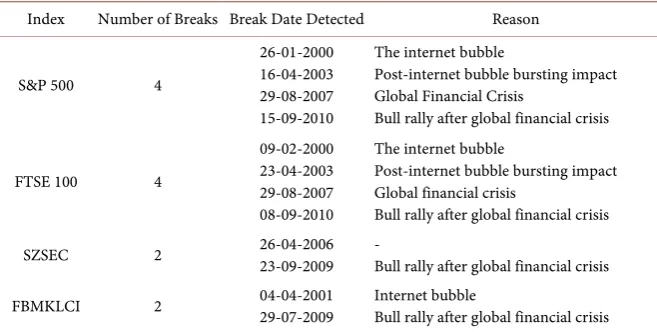
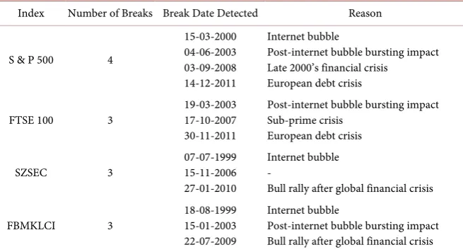
First, we identify the presence of volatility regimes in the AddRS estimator and the squared return using IT-ICSS approach. Table 2 and Table 3 report the breaks identified in the AddRS estimator and squared return respectively.

5.2. Estimation of the CARR Model Based on the AddRS and

GARCH Model Based on Returns

(6)

[image:6.595.208.540.89.267.2]

DOI: 10.4236/tel.2018.86080 1223 Theoretical Economics Letters Table 1. Descriptive statistics of the AddRS estimator (RS) and returns (rt).

AddRS Return

S&P 500 FTSE 100 SZSEC FBMKLCI S&P 500 FTSE 100 SZSEC FBMKLCI

Mean 1.270 1.444 1.755 1.132 0.119 0.063 0.156 0.039

Median 0.552 0.659 0.764 0.296 0.274 0.214 0.242 0.101

Min 0.008 0.014 0.000 0.001 −20.828 −15.297 −25.937 −13.720

Max 45.713 59.976 31.891 54.265 10.182 13.588 17.675 28.109

Stdev 2.634 3.016 3.039 3.308 2.363 2.390 3.704 2.938

Skewness 8.703# 9.901# 4.709# 9.100# −0.956# −0.441# −0.601# 1.269#

Kurtosis 116.428# 154.646# 33.133# 112.604# 10.627# 7.064# 8.109# 21.055#

JB stat 607965.2# 1079767.2# 46014.6# 569893.7# 2851.670# 797.433# 1270.789# 15332.112#

Q(20) 1149.728# 856.365# 596.870# 1280.295# 55.247# 42.985# 43.736# 83.904#

ARCH(10) 350.873# 138.080# 39.573# 245.005# 99.229# 121.457# 95.687# 124.006#

[image:6.595.208.537.332.498.2]

#means significant at 1% level. Note that Stdev represents the standard deviation, JB stat represents the Jarque Bera statistic, Q(20) indicates the Ljung-Box Q statistic up to 20 lags and ARCH(10) indicates the Lagrange multiplier test for conditional heteroskedasticity up to 10 lags.

Table 2. Breaks detected in the AddRS estimator.

Index Number of Breaks Break Date Detected Reason

S&P 500 4

26-01-2000 16-04-2003 29-08-2007 15-09-2010

The internet bubble

Post-internet bubble bursting impact Global Financial Crisis

Bull rally after global financial crisis

FTSE 100 4

09-02-2000 23-04-2003 29-08-2007 08-09-2010

The internet bubble

Post-internet bubble bursting impact Global financial crisis

SZSEC 2 26-04-2006 _23-09-2009 - _{Bull rally after global financial crisis}

FBMKLCI 2 04-04-2001 _29-07-2009 Internet bubble _{Bull rally after global financial crisis}

Equations (4) and (5). The models for incorporating the impact of structural breaks in squared return based on the GARCH model is given as:

( )

, ~ 0,1

t zt t zt N

ε = σ

2 2 2

1 1 1 1 1 1,

t d D d Dn n t t

σ = +ω + + +α ε− +β σ− (6) where D1,,Dn are the dummy variables taking a value of 1 for the given

vo-latility regime and 0 elsewhere.

The GARCH model without any volatility regimes is given as:

( )

, ~ 0,1

t zt t zt N

ε = σ

2 2 2

1 1 1 1,

t t t

σ = +ω α ε₋ +β σ₋ ₍₇₎

(7)

[image:7.595.209.537.89.267.2]

DOI: 10.4236/tel.2018.86080 1224 Theoretical Economics Letters Table 3. Breaks detected in the squared returns.

Index Number of Breaks Break Date Detected Reason

S & P 500 4

15-03-2000 04-06-2003 03-09-2008 14-12-2011

Internet bubble

Post-internet bubble bursting impact Late 2000’s financial crisis

European debt crisis

FTSE 100 3 19-03-2003 17-10-2007 30-11-2011

Post-internet bubble bursting impact Sub-prime crisis

European debt crisis

SZSEC 3 07-07-1999 15-11-2006 27-01-2010

Internet bubble -

FBMKLCI 3 18-08-1999 15-01-2003 22-07-2009

Internet bubble

Post-internet bubble bursting impact Bull rally after global financial crisis

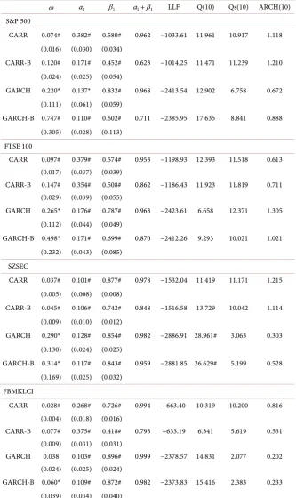
The standard errors of the parameters of the CARR models based on the AddRS estimator are smaller in magnitude than the standard errors of the cor-responding parameters from the GARCH models which confirms the finding of Brandt and Jones [15] regarding the unbiased and highly efficient nature of the extreme value volatility estimators. Results indicate that the short-term volatility component and long-term volatility components (based on significant values of

(8)

[image:8.595.207.541.102.663.2]

DOI: 10.4236/tel.2018.86080 1225 Theoretical Economics Letters Table 4. Parameter estimates of the CARR and GARCH models with and without volatil-ity breaks.

ω α1 β1 α1 + β1 LLF Q(10) Qs(10) ARCH(10) S&P 500

CARR 0.074# 0.382# 0.580# 0.962 −1033.61 11.961 10.917 1.118 (0.016) (0.030) (0.034)

CARR-B 0.120# 0.171# 0.452# 0.623 −1014.25 11.471 11.239 1.210 (0.024) (0.025) (0.054)

GARCH 0.220* 0.137* 0.832# 0.968 −2413.54 12.902 6.758 0.672 (0.111) (0.061) (0.059)

GARCH-B 0.747# 0.110# 0.602# 0.711 −2385.95 17.635 8.841 0.888 (0.305) (0.028) (0.113)

FTSE 100

CARR 0.097# 0.379# 0.574# 0.953 −1198.93 12.393 11.518 0.613 (0.017) (0.037) (0.039)

CARR-B 0.147# 0.354# 0.508# 0.862 −1186.43 11.923 11.819 0.711 (0.029) (0.039) (0.055)

GARCH 0.265* 0.176# 0.787# 0.963 −2423.61 6.658 12.371 1.305 (0.112) (0.044) (0.049)

GARCH-B 0.498* 0.171# 0.699# 0.870 −2412.26 9.293 10.021 1.021 (0.232) (0.043) (0.085)

SZSEC

CARR 0.037# 0.101# 0.877# 0.978 −1532.04 11.419 11.171 1.215 (0.005) (0.008) (0.008)

CARR-B 0.045# 0.106# 0.742# 0.848 −1516.58 13.729 10.042 1.114 (0.009) (0.010) (0.012)

GARCH 0.290* 0.128# 0.854# 0.982 −2886.91 28.961# 3.063 0.303 (0.130) (0.024) (0.025)

GARCH-B 0.314* 0.117# 0.843# 0.959 −2881.85 26.629# 5.199 0.528 (0.169) (0.025) (0.032)

FBMKLCI

CARR 0.028# 0.268# 0.726# 0.994 −663.40 10.319 10.200 0.816 (0.004) (0.018) (0.016)

CARR-B 0.077# 0.375# 0.418# 0.793 −633.19 6.341 5.619 0.531 (0.009) (0.031) (0.031)

GARCH 0.038 0.103# 0.896# 0.999 −2378.57 14.831 2.077 0.202 (0.024) (0.025) (0.024)

GARCH-B 0.060* 0.109# 0.872# 0.982 −2373.83 15.416 2.383 0.233 (0.039) (0.034) (0.040)

(9)

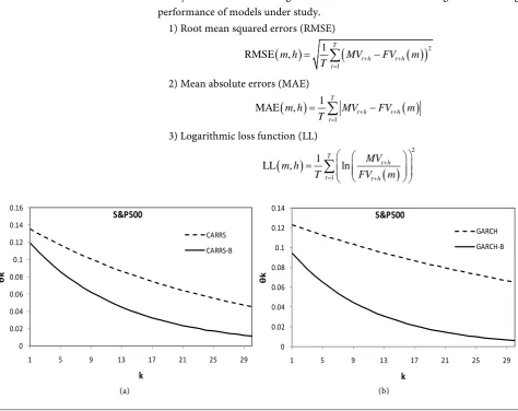
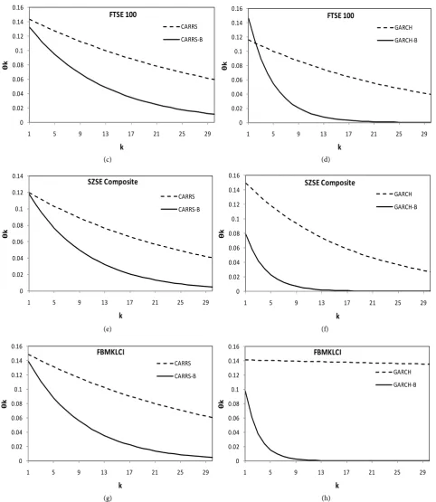
[image:9.595.62.537.363.739.2]

5.3. Dynamic Impulse Response Function Based on the CARR,

CARR-B, GARCH and GARCH-B Models

Figure 1 presents the dynamic impulse response functions for the CARR, CARR-B, GARCH and GARCH-B models with a forecast horizon up to 30 weeks. Results indicate that the response to a unit shock experience smooth de-cay for CARR-B model than for the vanilla CARR model. However, the response to a unit shock experience quick decay for the GARCH-B model than the GARCH model. This supports the evidence that the persistence in conditional volatility based on the CARR-B model remains for a longer period than the per-sistence in volatility based on the GARCH-B model. This also indicates the im-portance of incorporating structural breaks in volatility while modelling and fo-recasting volatility.

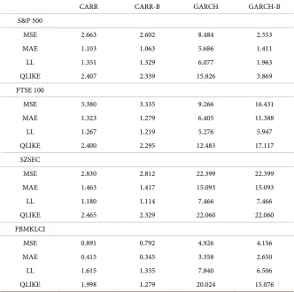
5.4. Out-of-Sample Volatility Forecast Comparison

In this section, we assess the forecasting performance of the models under study based on 1 step ahead prediction of volatility. The forecasts are generated using rolling windows estimation of the models with fixed window size. We generate 500 forecasts for all the models and for all the indices. We use weekly realized volatility (sum of the square of daily returns) based as a proxy for measured vo-latility. We use the following four loss functions for evaluating the forecasting performance of models under study.

1) Root mean squared errors (RMSE)

(

)

(

( )

)

2

1 1 RMSE ,

T

t h t h

t

m h MV FV m

T = + +

=

∑

−

2) Mean absolute errors (MAE)

(

)

( )

1 1

MAE ,

T

t h t h t

m h MV FV m

T = + +

=

∑

−

3) Logarithmic loss function (LL)

(

)

( )

2

1 1

LL , ln

T

t h

t t h

MV m h

T FV m

+ = +    = _ _ __    

∑

(a) (b) 0 0.02 0.04 0.06 0.08 0.1 0.12 0.14 0.16

1 5 9 13 17 21 25 29

θ k k S&P500 CARRS CARRS-B 0 0.02 0.04 0.06 0.08 0.1 0.12 0.14

1 5 9 13 17 21 25 29

(10)

(c) (d)

(e) (f)

[image:10.595.57.540.69.625.2]

(g) (h)

Figure 1. Dynamic impulse response function for the CARR and CARR-B models (left column) and the GARCH and GARCH-B

models (right column).

4) Loss implied by Gaussian likelihood (QLIKE)

(

)

(

( )

)

_{( )}

1 1

QLIKE , ln

T

t h t h

t t h

MV

m h FV m

T FV m

+ + = +   = _ + _  

∑

0 0.02 0.04 0.06 0.08 0.1 0.12 0.14 0.16

1 5 9 13 17 21 25 29

θ k k FTSE 100 CARRS CARRS-B 0 0.02 0.04 0.06 0.08 0.1 0.12 0.14 0.16

1 5 9 13 17 21 25 29

θ k k FTSE 100 GARCH GARCH-B 0 0.02 0.04 0.06 0.08 0.1 0.12 0.14

1 5 9 13 17 21 25 29

θ k k SZSE Composite CARRS CARRS-B 0 0.02 0.04 0.06 0.08 0.1 0.12 0.14 0.16

1 5 9 13 17 21 25 29

θ k k SZSE Composite GARCH GARCH-B 0 0.02 0.04 0.06 0.08 0.1 0.12 0.14 0.16

1 5 9 13 17 21 25 29

θ k k FBMKLCI CARRS CARRS-B 0 0.02 0.04 0.06 0.08 0.1 0.12 0.14 0.16

1 5 9 13 17 21 25 29

(11)

where m represents the model (CARR-B, CARR, GARCH-B and GARCH), h is equal to 1 representing 1 step ahead forecasts, MVt represents the measured vo-latility at time t (realized volatility), FVt(m) represents the predicted volatility based on model m and T represents the number of out-of-sample volatility fore-casts. Here, T is 500.

Table 5 reports the forecast evaluation results for all the models and indices under study. Results indicate that for all the indices, the CARR-B model provides more accurate forecasts than other models under consideration. More-over, the CARR model is at the second position to provide more accurate fore-casts of realized volatility for all the indices under study. The error statistics val-ue is quite high for both GARCH-B and GARCH models in comparison to CARR-B and CARR models.

5.5. Volatility Forecast Evaluation Based on Mincer and Zarnowitz

[20] Regression

In addition to the error statistics, we also use Mincer and Zarnowitz [20] regression-based approach to evaluate the ability of the models under study to generate more accurate forecasts of volatility. The regression model used is given as:

( )

t h t h t

MV₊ = +α βFV₊ m +ε

where MVt represents the measured volatility (realized volatility) at time t,

FVt(m) is a predicted volatility based on model m and εt represents the error term. Table 6 reports the R2_{of the Mincer and Zarnowitz}_[20]_regression equa-tion and it measures the total variaequa-tion in realized volatility explained by the predicted volatility. Results clearly indicate that the R2_{based on the CARR-B’s} predicted volatility is the highest for all the indices indicating the superior ability of the CARR-B model in generating more accurate forecasts of the volatility.

5.6. Trading Strategy to Study the Economic Significance of the

Study and Policy Implications

(12)

[image:12.595.206.539.90.420.2]

DOI: 10.4236/tel.2018.86080 1229 Theoretical Economics Letters Table 5. Out-of-sample volatility forecast evaluation.

CARR CARR-B GARCH GARCH-B

S&P 500

MSE 2.663 2.602 8.484 2.553

MAE 1.103 1.063 5.686 1.411

LL 1.351 1.329 6.077 1.963

QLIKE 2.407 2.339 15.826 3.869

FTSE 100

MSE 3.380 3.335 9.266 16.431

MAE 1.323 1.279 6.405 11.388

LL 1.267 1.219 5.276 5.947

QLIKE 2.400 2.295 12.483 17.117

SZSEC

MSE 2.830 2.812 22.399 22.399

MAE 1.463 1.417 15.093 15.093

LL 1.180 1.114 7.466 7.466

QLIKE 2.465 2.329 22.060 22.060

FBMKLCI

MSE 0.891 0.792 4.926 4.156

MAE 0.415 0.345 3.358 2.650

LL 1.615 1.335 7.840 6.506

QLIKE 1.998 1.279 20.024 15.076

Table 6. The R2_{based on the Mincer and Zarnowitz}_[20]_{regression model.}

S&P 500 0.407 0.418 0.286 0.295

FTSE 100 0.227 0.312 0.299 0.158

SZSEC 0.224 0.230 0.184 0.184

[image:12.595.209.539.573.663.2]

FBMKLCI 0.088 0.089 0.087 0.088

Table 7. Average annual return (%) for the risk-averse investor.

S & P 500 8.396 9.732 4.961 5.193

FTSE 100 4.106 4.817 −2.167 3.851

SZSEC 4.219 5.151 1.518 1.518

FBMKLCI 5.316 6.473 2.153 4.619

(13)

The findings of the study have implications towards policy maker, regulators, traders, risk managers, portfolio managers and investors. The study highlights the importance of incorporating structural breaks in volatility in modelling and in generating more accurate forecasts of volatility. The findings based on eco-nomic return earned by the risk-averse investor provide implication of the study for investors, traders and portfolio managers. Policy makers and regulators can use the unbiased AddRS volatility estimator in presence of structural breaks to understand the periods of stability and turbulence in the market and to imple-ment appropriate policies to deal with the adverse impact of any macroeconomic event. Moreover, more accurate forecasts of volatility in deriving more accurate Value-at-Risk and Expected Shortfall measures to quantify risk and has implica-tions for risk managers.

6. Conclusion

In this study, we propose the use of the CARR model to model the AddRS esti-mator and to generate a more accurate forecast of it. We also incorporate the impact of structural breaks in volatility in CARR model while modelling and fo-recasting the AddRS estimator. The results based on the in-sample estimation and impulse response support the evidence that incorporating the impact of structural breaks in volatility modelling does decrease the volatility persistence. We observe that this decrease in volatility persistence is smooth for CARR-B model. We observe an abrupt decrease in volatility persistence for the GARCH-B model. The results based on out-of-sample volatility forecast evaluation indicate that the CARR-B model provides more accurate forecasts of realized volatility when compared with corresponding volatility forecasts by another model. The economic significance analysis also indicates that the risk-averse investor can earn a higher average annualized return by trading based on the volatility fore-casts of the CARR-B model. Overall, our finding indicates that the CARR-B model outperforms other models in generating more accurate forecasts of rea-lized volatility.

References

[1] Kumar, D. and Maheswaran, S. (2014) A Reflection Principle for a Random Walk with Implications for Volatility Estimation Using Extreme Values of Asset Prices. Economic Modelling, 38, 33-44. https://doi.org/10.1016/j.econmod.2013.11.045 [2] Alizadeh, S., Brandt, M.W. and Diebold, F.X. (2002) Range-Based Estimation of

Stochastic Volatility Models. The Journal of Finance, 57, 1047-1091. https://doi.org/10.1111/1540-6261.00454

[3] Parkinson, M. (1980) The Extreme Value Method for Estimating the Variance of the Rate of Return. Journal of Business, 53, 61-65. https://doi.org/10.1086/296071 [4] Garman, M.B. and Klass, M.J. (1980) On the Estimation of Security Price

Volatili-ties from Historical Data. Journal of Business, 53, 67-78. https://doi.org/10.1086/296072

(14)

DOI: 10.4236/tel.2018.86080 1231 Theoretical Economics Letters Closing Prices. The Annals of Applied Probability, 1, 504-512.

https://doi.org/10.1214/aoap/1177005835

[6] Yang, D. and Zhang, Q. (2000) Drift-Independent Volatility Estimation Based on High, Low, Open, and Close Prices. The Journal of Business, 73, 477-492.

https://doi.org/10.1086/209650

[7] Kumar, D. and Maheswaran, S. (2012) Modelling Asymmetry and Persistence under the Impact of Sudden Changes in the Volatility of the Indian Stock Market. IIMB Management Review, 24, 123-136. https://doi.org/10.1016/j.iimb.2012.04.006 [8] Babikir, A., Gupta, R., Mwabutwa, C. and Owusu-Sekyere, E. (2012) Structural

Breaks and GARCH Models of Stock Return Volatility: The Case of South Africa. Economic Modelling, 29, 2435-2443. https://doi.org/10.1016/j.econmod.2012.06.038 [9] Rapach, D.E. and Strauss, J.K. (2008) Structural Breaks and GARCH Models of

Ex-change Rate Volatility. Journal of Applied Econometrics, 23, 65-90. https://doi.org/10.1002/jae.976

[10] Salisu, A.A. and Fasanya, I.O. (2013) Modelling Oil Price Volatility with Structural Breaks. Energy Policy, 52, 554-562. https://doi.org/10.1016/j.enpol.2012.10.003 [11] Ross, S.A. (1989) Information and Volatility: The No-Arbitrage Martingale

Ap-proach to Timing and Resolution Irrelevancy. The Journal of Finance, 44, 1-17. https://doi.org/10.1111/j.1540-6261.1989.tb02401.x

[12] Kumar, D. and Maheswaran, S. (2013) Evidence of Long Memory in the Indian Stock Market. Asia-Pacific Journal of Management Research and Innovation, 9, 9-21. https://doi.org/10.1177/2319510X13483504

[13] Inclan, C. and Tiao, G.C. (1994) Use of Cumulative Sums of Squares for Retrospec-tive Detection of Changes of Variance. Journal of the American Statistical Associa-tion, 89, 913-923.

[14] Chou, R.Y.T. (2005) Forecasting Financial Volatilities with Extreme Values: The Conditional Autoregressive Range (CARR) Model. Journal of Money, Credit, and Banking, 37, 561-582. https://doi.org/10.1353/mcb.2005.0027

[15] Brandt, M.W. and Jones, C.S. (2006) Volatility Forecasting with Range-Based EGARCH Models. Journal of Business & Economic Statistics, 24, 470-486. https://doi.org/10.1198/073500106000000206

[16] Kumar, D. (2015) Sudden Changes in Extreme Value Volatility Estimator: Model-ing and ForecastModel-ing with Economic Significance Analysis. Economic Modelling, 49, 354-371.https://doi.org/10.1016/j.econmod.2015.05.001

[17] Li, H. and Hong, Y. (2011) Financial Volatility Forecasting with Range-Based Au-toregressive Volatility Model. Finance Research Letters, 8, 69-76.

https://doi.org/10.1016/j.frl.2010.12.002

[18] Lamoureux, C.G. and Lastrapes, W.D. (1990) Persistence in Variance, Structural Change, and the GARCH Model. Journal of Business & Economic Statistics, 8, 225-234.

[19] Malik, F. (2003) Sudden Changes in Variance and Volatility Persistence in Foreign Exchange Markets. Journal of Multinational Financial Management, 13, 217-230. https://doi.org/10.1016/S1042-444X(02)00052-X