Efficient sampling of conditioned Markov jump processes

arXiv:1809.07139v2 [stat.CO] 30 Jan 2019

Efficient sampling of conditioned Markov jump processes

Andrew Golightly1∗, Chris Sherlock2

1_{School of Mathematics, Statistics and Physics, Newcastle University, UK} 2_{Department of Mathematics and Statistics, Lancaster University, UK}

Abstract

We consider the task of generating draws from a Markov jump process (MJP) between two time-points at which the process is known. Resulting draws are typically termedbridgesand the generation of such bridges plays a key role in simulation-based inference algorithms for MJPs. The problem is challenging due to the intractability of the conditioned process, necessitating the use of computationally intensive methods such as weighted resampling or Markov chain Monte Carlo. An efficient implementation of such schemes requires an approximation of the intractable conditioned hazard/propensity function that is both cheap and accurate. In this pa-per, we review some existing approaches to this problem before outlining our novel contribution. Essentially, we leverage the tractability of a Gaussian approximation of the MJP and suggest a computationally efficient implementation of the resulting conditioned hazard approximation. We compare and contrast our approach with existing methods using three examples.

Keywords: Markov jump process; conditioned hazard; chemical Langevin equation; linear noise

approximation

1

Introduction

Markov jump processes (MJPs) can be used to model a wide range of discrete-valued, continuous-time processes. Our focus here is on the MJP representation of a reaction network, which has been ubiquitously applied in areas such as epidemiology (Fuchs, 2013; Lin and Ludkovski, 2013; McKinley et al., 2014), population ecology (Matis et al., 2007; Boys et al., 2008) and systems biol-ogy (Wilkinson, 2009, 2018; Sherlock et al., 2014). Whilst exact, forward simulation of this class of MJP is straightforward (Gillespie, 1977), the reverse problem of performing fully Bayesian inference for the parameters governing the MJP given partial and/or noisy observations is made challenging by the intractability of the observed data likelihood. Simulation-based approaches to inference typically involve “filling in” event times and types between the observation times. A key repeated step in many inference mechanisms starts with a sample of possible states at one observation time and for each element of the sample, creates a trajectory starting with the sample value and ending at the time of the next observation with a value that is consistent with the next observation. The resulting conditioned samples are typically referred to as bridges, and ideally the bridge should be a draw from the exact distribution of the path given the initial condition and the observation. However, except for a few simple cases, exact simulation of MJP bridges is infeasible, necessitat-ing approximate bridge constructs that can be used as a proposal mechanism inside a weighted resampling and/or Markov chain Monte Carlo (MCMC) scheme.

The focus of this paper is the development of an approximate bridge construct that is both accurate and computationally efficient. Our contribution can be applied in a generic observation regime that allows for discrete, partial and noisy measurements of the MJP, and is particularly

effective compared to competitors in the most difficult regime where the observations are sparse in time and the observation variance is small. Many bridge constructs have been proposed for partially observed stochastic differential equations (SDEs, e.g. Delyon and Hu (2006), Bladt and Sørensen (2014), Bladt et al. (2016), Schauer et al. (2017) and Whitaker et al. (2017)) but the literature on bridges for MJPs is relatively sparse. Recent progress involves an approximation of the instanta-neous rate or hazard function governing the conditioned process. For example, Boys et al. (2008) linearly interpolate the hazard between observation times but require full and error-free observa-tion of the system of interest. Fearnhead (2008) recognises that the condiobserva-tioned hazard requires the intractable transition probability mass function of the MJP. This is then directly approxi-mated by substituting the transition density associated with the coarsest possible discretisation of a spatially continuous approximation of the MJP, the chemical Langevin equation (Gillespie, 2000). Golightly and Wilkinson (2015) derive a conditioned hazard by approximating the expected number of events between observations, given the observations themselves. Unfortunately, the latter two approaches typically perform poorly when the behaviour of the conditioned process is nonlinear.

We take the approach of Fearnhead (2008) as a starting point and replace the intractable MJP transition probability with the transition density governing the linear noise approximation (LNA) (Kurtz, 1970; Elf and Ehrenberg, 2003; Komorowski et al., 2009; Schnoerr et al., 2017). Whilst the LNA has been used as an inferential model (see e.g. Ruttor and Opper (2009) and Ruttor et al. (2010) for a maximum likelihood approach and Stathopoulos and Girolami (2013) and Fearnhead et al. (2014) for an MCMC approach), we believe that this is the first attempt to use the LNA to develop a bridge construct for simulation of conditioned MJPs. We find that the LNA offers superior accuracy over a single step of the CLE (which must be discretised in practice), at the expense of computational efficiency. Notably, the LNA solution requires, for each event time in each trajectory, integrating forwards until the next event time a system of ordinary differential equations (ODEs) whose dimension is quadratic in the number of MJP components. We therefore leverage the linear Gaussian structure of the LNA to derive a bridge construct that only requires a single full integration of the LNA ODEs, irrespective of the number of transition events on each bridge or the number of bridges required. We compare the resulting novel construct to several existing approaches using three examples of increasing complexity. In the final, real-data applica-tion, we demonstrate use of the construct within a pseudo-marginal Metropolis-Hastings scheme, for performing fully Bayesian inference for the parameters governing an epidemic model.

The remainder of this paper is organised as follows. In Section 2 we define a Markov jump process as a probabilistic description of a reaction network. We consider the task of sampling con-ditioned jump processes in Section 3, and review two existing approaches. Our novel contribution is presented in Section 4 and illustrated in Section 5. Conclusions are drawn in Section 6.

2

Reaction networks

Consider a reaction network involvinguspeciesX1,X2, . . . ,Xuandv reactionsR1,R2, . . . ,Rv such

that reaction Ri is written as

u X

j=1

aijXj −→ u X

j=1

bijXj, i= 1, . . . , v

where aij denotes the number of molecules of Xj consumed by reaction Ri and bij denotes the

number of molecules of Xj produced by reaction Ri. Let Xj,t denote the (discrete) number of

species Xj at time t, and let Xt be the u-vector Xt = (X1,t, X2,t, . . . , Xu,t)′. The effect of a

Algorithm 1 Gillespie’s direct method

1. Sett= 0. Initialise withx0 = (x1,0, . . . , xu,0)′.

2. Calculate hi(xt), i= 1, . . . , v and the combined hazard h0(xt) =Pv_i=1hi(xt).

3. Simulate the time to the next event, t′_∼Exp(h

0(xt)).

4. Simulate the reaction index,i, as a discrete random quantity with probabilityhi(xt)/h0(xt),

i= 1, . . . , v.

5. Putxt+t′ :=x_t+Si, whereSi denotes theith column of S.

6. Putt:=t+t′. Outputxtand t. Ift < T, return to step 2.

reaction occurs at time t, the new state becomes

Xt=Xt−+Si

where Si _{= (b}

i1−ai1, . . . , biu−aiu)′ is the ith column of the u×v stoichiometry matrix S. The

time evolution of Xt is therefore most naturally described by a continuous-time, discrete-valued

Markov process defined in the following section.

2.1 Markov jump processes

We model the time evolution of Xt via a Markov jump process (MJP), so that the state of the

system at time tis

Xt=x0+

X

i

SiRi,t

where x0 is the initial system state and Ri,t denotes the number of times that the ith reaction

occurs by timet. The processRi,t is a counting process with intensityhi(xt), known in this setting

as the reaction hazard, which depends on the current state of the system xt. Explicitly, we have

that

Ri,t =Yi

Z t

0

hi(xs)ds

where the Yi, i= 1, . . . , v are independent, unit rate Poisson processes (see e.g. Kurtz (1972) or

Wilkinson (2018) for further details of this representation). The hazard function is given byh(xt) =

(h1(xt), . . . , hv(xt))′. Under the standard assumption of mass-action kinetics, hi is proportional to

a product of binomial coefficients. That is

hi(xt) =ci u Y

j=1

xj,t

aij

whereci is the rate constant associated with reactionRi and c= (c1, c2, . . . , cv)′ is a vector of rate

constants. Since in this article, except in Section 5.3 the rate constants are assumed to be a known fixed quantities we drop them from the notation where possible.

3

Sampling conditioned MJPs

Denote by X = {Xs|0 < s ≤ T} the MJP sample path over the interval (0, T]. Complete

information on an observed sample path x corresponds to all reaction times and types. To this

end, let nr denote the total number of reaction events; reaction times (assumed to be in increasing

order) and types are denoted by (ti, νi), i = 1, . . . , nr, νi ∈ {1, . . . , v} and we take t0 = 0 and

tnr+1=T.

Suppose that the initial state x0 is a known fixed value and that (a subset of components of)

the process is observed at timeT subject to Gaussian error, giving a single observation yT on the

random variable

YT =P′xT +εT , εT ∼N (0,Σ). (1)

Here, YT is a length-d vector, P is a constant matrix of dimension u×d and εT is a length-d

Gaussian random vector. The role of the matrix P is to provide a flexible setup allowing for

various observation scenarios. For example, taking P to be theu×u identity matrix corresponds to the case of observing all components ofXt(subject to error). We denote the density linking YT

and XT asp(yT|xT).

We consider the task of generating trajectories from p(x|x0, yT) given by

p(x|x0, yT) =

p(yT|xT)p(x|x0)

p(yT|x0)

∝p(yT|xT)p(x|x0) (2)

Here,p(x|x0) is the complete data likelihood (Wilkinson, 2018) which takes the form

p(x|x0) =

(Y_nr

i=1

hνi xti₋1

)

exp

−

Z T

0

h0(xt)dt

whereh0 is as defined in line 2 of Algorithm 1. Although p(x|x0, yT) will typically be intractable,

generating draws fromp(x|x0) is straightforward via Gillespie’s direct method (Algorithm 1). This

immediately suggests drawing samples from (2) using a numerical scheme such as weighted resam-pling. However, as discussed in Golightly and Wilkinson (2015), drawing unconditioned trajectories fromp(x|x0) and weighting byp(yT|xT) is likely to lead to highly variable weights, unless the level

of intrinsic stochasticity of Xt is outweighed by the variance of the observation process. Our

um-brella aim, therefore, is to find an approximating MJP whose dynamics remain tractable under conditioning on yT. The resulting construct can then be used to generate proposed trajectories

within the weighted resampling scheme. We will show that this is possible via the derivation of an approximate conditioned hazard function, ˜h(xt|yT),t∈(0, T], that can be used in place of h(xt) in

Algorithm 1. The form for ˜h(xt|yT) that we initially derive depends explicitly ont, so that sampling

events might not be straightforward; however the time-dependence is sufficiently small that it can be ignored and the resulting bridge mechanism, which has a constant rate between events, still leads to efficient proposals.

3.1 Weighted resampling

Letq(x|x0, yT) denote the complete data likelihood for a sample pathxdrawn from an approximate

jump process with hazard function ˜h(xt|yT). The importance weight associated with xis given by

w(x) =p(yT|xT)

dP

dQ(x)

Algorithm 2 Weighted resampling for MJPs

1. Forj= 1,2, . . . , N:

(a) Draw xj ∼q(x|x0, yT) using Algorithm 1 withh(xt) replaced by ˜h(xt|yT).

(b) Construct the unnormalised weight

˜

wj := ˜w xj=p(yT|xj_T)

p(xj|x0)

q(xj|x0, yT)

whose form is given by (3).

(c) Normalise the weights: wj _{= ˜w}j_/PN i=1w˜i.

2. Resample (with replacement) from the discrete distribution on x1, . . . ,xN using the nor-malised weights as probabilities.

An informal approach is provided by Wilkinson (2018), giving the Radon-Nikodym derivative as the likelihood ratio

dP

dQ(x) =p(yT|xT)

(_nr Y

i=1

hνi xti₋1

˜

hνi xti₋1|yT

)

exp

−

Z T

0

h

h0(xt)−h˜0(xt|yT) i

dt

where h0(xt) = Pvi=1hi(xt) and ˜h0(xt|yT) is defined analogously. As noted above, the explicit

dependence of ˜h on t is ignored so that bothh0 and ˜h0 are piece-wise constant (between reaction

events). Hence, in practice, we evaluate the weight using

w(x) =p(yT|xT) (_nr

Y

i=1

hνi xti−1

˜

hνi xti₋1|yT

)

exp

( −

nr

X

i=0

h

h0(xti)−h˜0(xti|yT)

i

∆ti )

(3)

where ∆ti =ti+1−ti.

The general weighted resampling algorithm is given by Algorithm 2. It is straightforward to show that the average unnormalised weight gives an unbiased estimator of the transition density p(yT|x0). This estimator is given by

ˆ

p(yT|x0) =

1 N

N X

j=1

p(yT|XTj)

p(Xj|x0)

q(Xj|x0, yT)

(4)

whereXj is an independent draw fromq(·|x0, yT). In the case of an unknown initial valueX0 with

density p(x0), Algorithm 2 can be initialised with a sample of size N from p(x0) in which case (4)

can be used to estimate p(yT).

It remains for us to find a suitable form of ˜h(xt|yT). In what follows, we review two existing

methods before presenting a novel, alternative approach. Comparisons are made in Section 5.

3.2 Golightly and Wilkinson approach

The approach of Golightly and Wilkinson (2015) is based on a (linear) Gaussian approximation of the number of reaction events in the time between the current event time and the next observation time. Suppose we have simulated as far as timetand let ∆Rtdenote the number of reaction events

reaction hazard over the whole non-infinitesimal time interval, ∆t. A Gaussian approximation to the corresponding Poisson distribution then gives

∆Rt∼N (h(xt)∆t , H(xt)∆t)

whereH(xt) = diag{h(xt)}. Under the Gaussian observation regime given by (1) it should be clear

that the joint distribution of ∆Rt andYT can then be approximated by

∆Rt

YT

∼N

h(xt)∆t

P′_(x

t+S h(xt)∆t)

,

H(xt)∆t H(xt)S′P∆t

P′_{S H(x}

t)∆t P′S H(xt)S′P∆t+ Σ

.

Taking the expectation of (∆Rt|YT = yT) and dividing by ∆t gives an approximate conditioned

hazard as

˜

h(xt|yT) =h(xt)

+H(xt)S′P P′S H(xt)S′P∆t+ Σ−1 yT −P′[xt+S h(xt)∆t]. (5)

By ignoring the explicit time dependence of ˜h(xt|yT) (i.e., after each most-recent event, until the

next event, fixing ∆t to its value at the most recent event), we can use (5), suitably truncated to ensure positivity, in Algorithm 1 to give trajectories xi,i = 1, . . . , N, to be used in Algorithm 2. Whilst use of (5) has been shown to work well in several applications, assumptions of normality of ∆Rt and that the hazard is constant over a time interval of length ∆t are often unreasonable, as

we will show.

3.3 Fearnhead approach

As noted by Fearnhead (2008) (see also Ruttor and Opper (2009)), an expression for the intractable conditioned hazard can be derived exactly. Consider again an interval [0, T] and suppose that we have simulated as far as timet∈[0, T]. For reactionRi letx′ =xt+Si. Recall thatSi denotes the

ith column of the stoichiometry matrix so thatx′ _{is the state of the MJP after a single occurrence} of Ri. The conditioned hazard of Ri satisfies

hi(xt|yT) = lim δt→0

P r(Xt+δt=x′|Xt =xt, yT)

δt

=hi(xt) lim δt→0

p(yT|Xt+δt=x′)

p(yT|Xt=xt)

=hi(xt)

p(yT|Xt=x′)

p(yT|Xt=xt)

. (6)

In practice, the intractable transition densityp(yT|xt) must be replaced by a suitable approximation.

Golightly and Kypraios (2017) (see also Fearnhead (2008) for the case of no measurement error) used the transition density governing the (discretised) chemical Langevin equation (CLE). The CLE (Gillespie, 1992, 2000) is an Itˆo stochastic differential equation (SDE) that has the same infinitesimal mean and variance as the MJP. It is written as

dXt=S h(Xt)dt+ p

Sdiag{h(Xt)}S′dWt, (7)

where Wt is au-vector of standard Brownian motion and p

Sdiag{h(Xt)}S′ is a u×u matrix B

such that BB′ =Sdiag{h(Xt)}S′. Since the CLE can rarely be solved analytically, it is common

to work with a discretisation such as the Euler-Maruyama discretisation:

Xt+δt−Xt=S h(Xt)δt+ p

whereZ is a standard multivariate Gaussian random variable. Combining (8) with the observation model (1) gives an approximate conditioned hazard as

˜

hi(xt|yT) =hi(xt)

pcle(yT|Xt =x′)

pcle(yT|Xt=xt)

(9)

where

pcle(yT|Xt=xt) =N yT;P′(xt+S h(xt)∆t), P′S H(xt)S′P∆t+ Σ

with pcle(yT|Xt =x′) defined similarly. As with the approach of Golightly and Wilkinson (2015),

the remaining time ∆t until the observation is treated as a single discretisation. However, unless ∆t= T −t is very small, pcle is unlikely to achieve a reasonable approximation of the transition

probability under the jump process. In what follows, therefore, we seek an approximation that is both accurate and computationally inexpensive.

4

Improved constructs

We take (6) as a starting point and replace p(yT|Xt = x′) and p(yT|Xt = xt) using the

lin-ear noise approximation (LNA) (Kurtz, 1970; Elf and Ehrenberg, 2003; Komorowski et al., 2009; Schnoerr et al., 2017). We first describe the LNA, and then consider two constructions for bridges from a known initial condition, x0, to a potentially noisy observation YT, based on different

im-plementations of the LNA. The first is expected to be more accurate as the approximate hazard is recalculated after every event by re-integrating a set of ODEs from the event time to the obser-vation time both from the current value and once for each possible next reaction. The second is more computationally efficient as the recalculation is based on a single, initial integration of a set

of ODEs from time 0 to time T.

4.1 Linear noise approximation

For notational simplicity we rewrite the CLE in (7) as

dXt=α(Xt)dt+ p

β(Xt)dWt (10)

where

α(Xt) =S h(Xt), β(Xt) =Sdiag{h(Xt)}S′

and derive the LNA by directly approximating (10). The basic idea behind construction of the LNA is to adopt the partitionXt=zt+Mtwhere the deterministic processzt satisfies an ordinary

differential equation

dzt

dt =α(zt) (11)

and the residual stochastic processMtcan be well approximated under the assumption that residual

stochastic fluctuations are “small” relative to the deterministic process. Taking the first two terms in the Taylor expansion ofα(Xt), and the first term in the Taylor expansion ofβ(Xt) gives an SDE

satisfied by an approximate residual process ˜Mt of the form

dM˜t=FtM˜tdt+ p

β(zt)dWt, (12)

whereFtis the Jacobian matrix with (i, j)th element (Ft)i,j =∂αi(zt)/∂zj,t. The SDE in (12) can

be solved by first defining the u×u fundamental matrix Gt as the solution of

dGt

whereIu is theu×uidentity matrix. Under the assumption of a fixed or Gaussian initial condition,

˜

M0 ∼N(m0, V0), it can be shown that (see e.g. Fearnhead et al., 2014)

˜

Mt|M˜0 =m0∼N(Gtm0, GtψtG′t)

whereψt satisfies

dψt

dt =G −1

t β(zt, c) G−t1 ′

. (14)

It is convenient here to writeVt=GtψtG′t and it is straightforward to show that Vt satisfies

dVt

dt =VtF ′

t+β(zt, c) +FtVt. (15)

In practice, ifx0 is a known fixed value then we may takez0=x0,m0 = 0u (theu-vector of zeros)

andV0 = 0u×u (theu×u zero matrix). Solving (11) and (15) gives the approximating distribution

of Xt as

Xt|X0 =x0∼N(zt, Vt).

In this case, the ODE system governing the fundamental matrix Gt need not be solved.

4.2 LNA bridge with restart

Now, consider again the problem of approximating the MJP transition probability p(yT|Xt =xt).

Given a value xt at time t ∈[0, T), the ODE system given by (11) and (15) can be re-integrated

over the time interval (t, T] to give output denoted byzT|tandVT|t. Similarly, the initial conditions

are denoted z_t|t =xt and Vt|t = 0u×u. We refer to use of the LNA in this way as the LNA with

restart (LNAR). The approximation top(yT|Xt=xt) is given by

plnar(yT|Xt=xt) =N yT;P′zT|t, P′VT|tP + Σ

.

Likewise,plnar(yT|Xt=x′) can be obtained by initialising (11) withzt|t=x′ and integrating again.

Hence, the approximate conditioned hazard is given by

˜

hi(xt|yT) =hi(xt)

plnar(yT|Xt=x′)

plnar(yT|Xt=xt)

(16)

Whilst use of the LNA in this way is likely to give an accurate approximation to the intractable transition probability (especially ast approachesT), the conditioned hazard in (6) must be calcu-lated forxt and for each x′ obtained after the v possible transitions of the process. Consequently,

the ODE system given by (11) and (15) must be solved at each event time for each of the v+ 1

possible states. Since the LNA ODEs are rarely tractable (necessitating the use of a numerical solver), this approach is likely to be prohibitively expensive, computationally. In the next section, we outline a novel strategy for reducing the cost associated with integrating the LNA ODE system, that only requires one full integration.

4.3 LNA bridge without restart

Consider the solution of the ODE system given by (11), (13) and (14) over the interval (0, T] with respective initial conditions Z0 = x0, G0 =Iu and ψ0 = 0u×u. Although in practice a numerical

Given a value xt at time t ∈ [0, T), the LNA (without restart) approximates the intractable

transition probability under the MJP by

plna(yT|Xt =xt) =N yT;P′[zT +GT|t(xt−zt)], P′[GT|tψT|tG′T|t]P + Σ

whereGT|tand ψT|t are the solutions of (13) and (14) integrated over (t, T] with initial conditions

G_t|t=Iu andψt|t= 0u×u. Crucially, the ODE system satisfied byztis not re-integrated (and hence

the residual term at time t is ˜Mt = xt−zt). Moreover, GT|t and ψT|t can be obtained without

further integration. We have that

E( ˜MT|M˜0 =m0) =GTm0

=G_T|tE( ˜Mt|M˜0=m0)

=GT|tGtm0

and therefore the first identity we require is

G_T|t=GTG−t1. (17)

Similarly,

Var( ˜MT|M˜0 =m0) =GTψTGT

=G_T|tVar( ˜Mt|M˜0 =m0)G′T|t

+GT|tψT|tG′T|t

=GTψtG′T +GT|tψT|tG′T|t

=GTψtG′T +GTGt−1ψT|t(G′t)−1G′T

where we have used (17) to obtain the last line. The second identity we require is therefore

ψT|t=Gt(ψT −ψt)G′t. (18)

Hence, given zt, Gt and ψt for t ∈ (0, T], plna(yT|Xt = xt, c) is easily evaluated via repeated

application of (17) and (18). Additionally obtainingplna(yT|Xt=x′) is straightforward by replacing

the residualxt−zt withx′−zt. Hence, only one full integration of (11), (13) and (14) over (0, T]

is required, giving a computationally efficient construct. The conditioned hazard takes the form

˜

hi(xt, c|yT) =hi(xt)

plna(yT|Xt=x′)

plna(yT|Xt=xt)

(19)

In Section 6 we describe how, in the case of unknownX0it is possible to make further computational

savings, using this technique.

The accuracy ofplna(and therefore the accuracy of the resulting conditioned hazard) is likely to

depend onT, the length of the inter-observation period over which a realisation of the conditioned process is required. For example, the residual process ˜Mt will approximate the true (intractable)

residual process increasingly poorly if zt andXtdiverge significantly astincreases. We investigate

the effect of inter-observation time in the next section.

5

Applications

stochastic Lotka-Volterra model examined by Boys et al. (2008) among others and a susceptible-infected-removed (SIR) epidemic model. For the last of these, we use the best performing LNA-based construct to drive a pseudo-marginal Metropolis-Hastings (PMMH) scheme to perform fully Bayesian inference for the rate constantsc. Using real data consisting of susceptibles and infectives during the well studied Eyam plague (Raggett, 1982), we compare bridge-based PMMH with a standard implementation (using blind, forward simulation) and a recently proposed scheme based on the alive particle filter (Drovandi et al., 2016). All algorithms are coded in R and were run on a desktop computer with an Intel Core i7-4770 processor at 3.40GHz.

5.1 Death model

We consider a single reaction, governing a single specie X, of the form

R1 : X −→ ∅

with associated hazard function

h(xt) =c xt

wherext denotes the state of the system at timet.

Under the assumption of an error free observation scenario, the conditioned hazard of Golightly and Wilkinson (2015), given by (5), takes the form

˜

h(xt|yT) =

xT −xt

∆t

and recall that ∆t=T −t. The CLE is given by

dXt=−c Xtdt+ p

c XtdWt.

Although the CLE is tractable in this special case (Cox et al., 1985), for reaction networks of reasonable size and complexity, the CLE will be intractable. We therefore implement the approach of Fearnhead (2008) by taking the conditioned hazard as in (9) wherepcleis based on a single-time

step numerical approximation of the CLE. The Euler-Maruyama approximation gives

pcle(xT|xt) =N(xt;xt−c xt∆t , c xt∆t).

The ODE system characterising the LNA (equations (11), (13) and (14)) with respective initial conditionsz0 =x0,G0 =Iu and ψ0 = 0u×u can be solved analytically to give

zt=x0e−c t, Gt=e−c t, ψt=x0 ec t−1.

Hence, for the LNA with restart, we have that

plnar(xT|xt) =NxT ;xte−c∆t, xte−c∆t 1−e−c∆t .

For the LNA without restart, we obtain

plna(xT|xt) =NxT;xte−c∆t, x0e−c T 1−e−c∆t .

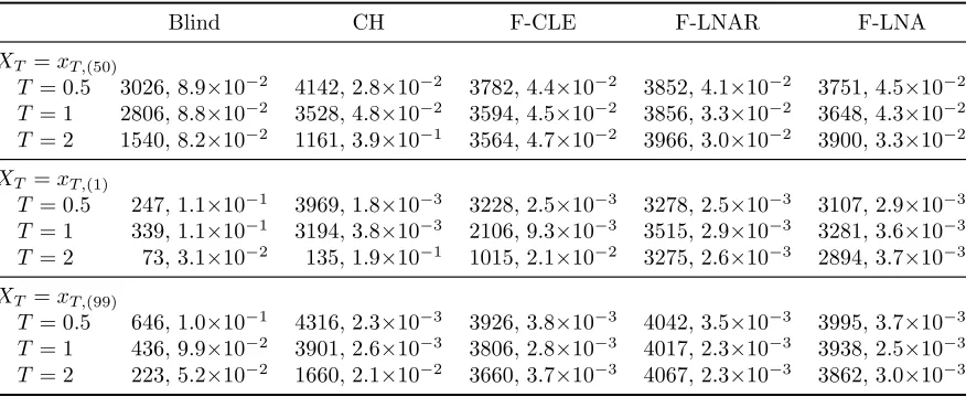
In what follows, we took c = 0.5 and x0 = 50 to be fixed. The end-point xT was chosen

as either the median, lower 1% or upper 99% quantile of the forward process XT|X0 = 50. We

adopt the notation that x_T,(α) is the α% quantile of XT|X0 = 50. Hence, we took the

end-point xT ∈ {xT,(1), xT,(50), xT,(99)}. To assess the performance of the proposed approach as an

Blind CH F-CLE F-LNAR F-LNA

XT =xT,(50)

T = 0.5 3026, 8.9×10−2 _{4142, 2.8×10}−2 _{3782, 4.4×10}−2 _{3852, 4.1×10}−2 _{3751, 4.5×10}−2

T = 1 2806, 8.8×10−2 _{3528, 4.8×10}−2 _{3594, 4.5×10}−2 _{3856, 3.3×10}−2 _{3648, 4.3×10}−2

T = 2 1540, 8.2×10−2 _{1161, 3.9×10}−1 _{3564, 4.7×10}−2 _{3966, 3.0×10}−2 _{3900, 3.3×10}−2

XT =xT,(1)

T = 0.5 247, 1.1×10−1 _{3969, 1.8×10}−3 _{3228, 2.5×10}−3 _{3278, 2.5×10}−3 _{3107, 2.9×10}−3

T = 1 339, 1.1×10−1 _{3194, 3.8×10}−3 _{2106, 9.3×10}−3 _{3515, 2.9×10}−3 _{3281, 3.6×10}−3

T = 2 73, 3.1×10−2 _{135, 1.9×10}−1 _{1015, 2.1×10}−2 _{3275, 2.6×10}−3 _{2894, 3.7×10}−3

XT =xT,(99)

T = 0.5 646, 1.0×10−1 _{4316, 2.3×10}−3 _{3926, 3.8×10}−3 _{4042, 3.5×10}−3 _{3995, 3.7×10}−3

T = 1 436, 9.9×10−2 _{3901, 2.6×10}−3 _{3806, 2.8×10}−3 _{4017, 2.3×10}−3 _{3938, 2.5×10}−3

T = 2 223, 5.2×10−2 _{1660, 2.1×10}−2 _{3660, 3.7×10}−3 _{4067, 2.3×10}−3 _{3862, 3.0×10}−3

Table 1: Death model. ESS(_bπ1:m) and ReMSE(π_b1:m), based on 5000 runs of each algorithm.

hazard function, the conditioned hazard of Golightly/Wilkinson given by (5), and the Fearnhead approach based on the CLE (9), LNA with restart (16) and LNA without restart (19). The resulting

algorithms are designated as blind, GW, F-CLE, F-LNAR and F-LNA. Each was run m = 5000

times with N = 10 samples to give a set of 5000 estimates of the transition probability π(xt|x0)

and we denote this set by _bπ1:m(xt|x0). To compare the algorithms, we report the effective sample

size

ESS(_bπ1:m) =

Pm i=1πbi

2

Pm i=1(πbi)

2

and relative mean-squared error ReMSE(π_b1:m) given by

ReMSE(_bπ1:m) = 1 m

m X

i=1

b

πi(xt|x0)−π(xt|x0)2

π(xt|x0)

whereπ(xt|x0) can be obtained analytically (e.g., Bailey (1964)) as

π(xt|x0) =

x0

xt

e−c t xt

1−e−c tx0−xt

.

The results are summarised in Table 1. Whilst the Blind approach gives broadly comparable performance to the conditioned approaches whenxT =xT,(50), its performance deteriorates

signifi-cantly when the end-point is taken to be a value in the tails ofxt|X0 = 50. This is due to the Blind

approach struggling to generate trajectories that are highly unlikely to hit the neighbourhood of the end-point. For the CH approach we see a decrease in ESS and an increase in ReMSE asT increases, due to the linear form being unable to adequately describe the exponential like decay exhibited by

the true conditioned process. Whilst the F-CLE approach performs well when xT = xT,(50) and

xT =xT,(99), it is unable to match the performance of the LNA-based methods across all scenarios.

T = 1 T = 2 T = 3 T = 4

yT,(1) (53.34, 27.99) (75.83, 22.59) (109.51, 20.90) (157.34, 23.65)

yT,(50) (73.25, 58.43) (108.69, 39.92) (162.03, 41.23) (238.62, 49.89)

yT,(99) (95.33, 58.43) (147.28, 58.26) (225.77, 64.19) (337.65, 83.79)

Table 2: Lotka-Volterra model. Quantiles ofYT|X0 = (50,50)′ found by repeatedly simulating from

the Euler-Maruyama approximation of (20) with c = (0.5,0.0025,0.3)′ _{and corrupting X}

1,T and

X2,T with additive N(0,52) noise.

5.2 Lotka-Volterra

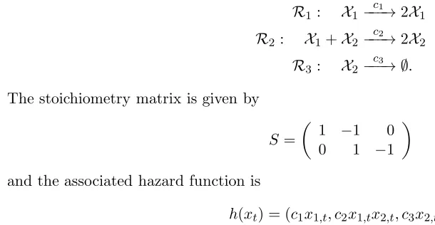
We consider here a Lotka-Volterra model of prey (X1) and predator (X2) interaction comprising

three reactions of the form

R1: X1−−−→c1 2X1

R2 : X1+X2 c 2

−−−→2X2

R3: X2 c 3

−−−→ ∅.

The stoichiometry matrix is given by

S =

1 −1 0

0 1 −1

and the associated hazard function is

h(xt) = (c1x1,t, c2x1,tx2,t, c3x2,t)′.

The conditioned hazard described in Section 3.2 and given by (5) can then be obtained. The CLE for the Lotka-Volterra model is given by

d

X1

X2

=

c1X1−c2X1X2

c2X1X2−c3X2

dt+

c1X1+c2X1X2 −c2X1X2

−c2X1X2 c2X1X2+c3X2

1/2

d

W1

W2

(20)

after suppressing dependence on t. It is then straightforward to obtain the Euler-Maruyama

ap-proximation of the CLE, for use in the conditioned hazard described in Section 3.3 and given by (9).

For the linear noise approximation, the Jacobian matrix Ft is given by

Ft=

c1−c2z2,t −c2z1,t

c2z2,t c2z1,t−c3

.

Unfortunately, the ODEs characterising the LNA solution, given by (11), (13) and (14) are in-tractable, necessitating the use of a numerical solver. In what follows, we use thedeSolve package in R, with the default lsoda integrator (Petzold, 1983).

Our initial experiments used the following settings. Following Boys et al. (2008) among others we imposed the parameter values c = (c1, c2, c3)′ = (0.5,0.0025,0.3)′ and let x0 = (50,50)′. We

assumed an observation model of the form (1) and took Σ = σ2_I

2 with σ = 5 representing low

measurement error (since typical simulations of X1,t and X2,t are around two orders of magnitude

larger thanσ). We generated a number of challenging scenarios by takingyT as the pair of 1%, 50%

or 99% marginal quantiles ofYT|X0= (50,50)′ forT ∈ {1,2,3,4}. These quantiles are denoted by

y_T,(1),y_T,(50) and y_T,(99) respectively, and are shown in Table 2.

0 1 2 3 4 0 50 100 150 200 250 300 350

0 1 2 3 4

0 50 100 150 200 250 300 350

0 1 2 3 4

0 50 100 150 200 250 300 350 P S fr ag re p la ce m en ts

CH F-LNAR F-LNA

F -C L E B lin d Xt Xt Xt t t t

0 1 2 3 4

0 50 100 150 200 250 300 350

0 1 2 3 4

0 50 100 150 200 250 300 350 P S fr ag re p la ce m en ts C H F -L N A F -L N A R F-CLE Blind Xt Xt t t

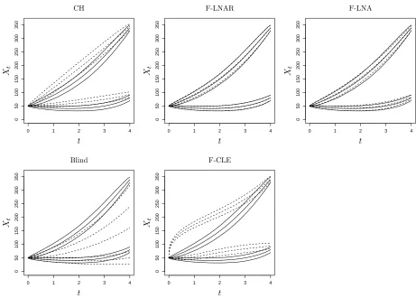
Figure 1: Lotka-Volterra model. Mean and two standard deviation intervals for the true conditioned processXt|x0, yT (solid lines) and various bridge constructs (dashed lines) usingyT =yT,(99),T = 4

and σ = 5. The upper lines correspond to the prey component and the lower lines correspond to

the predator component.

for the extreme case ofT = 4 andyT =yT,(99). Plainly, the blind forward simulation approach and

CLE-based Fearnhead approach (F-CLE) are unable to match the dynamics of the true conditioned

process. Moreover, we found that these bridges gave very small effective sample sizes for T ≥ 2

and we therefore omit these results from the following analysis.

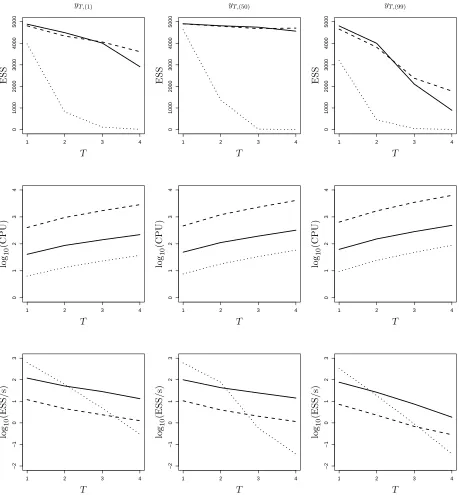
We report results based on weighted resampling using N = 5000 with three different hazard

functions: the Golightly/Wilkinson approach (CH) and the Fearnhead approach based on the LNA with and without restart (F-LNAR and F-LNA respectively). For the latter (F-LNA), we integrated the LNA once in total. Figure 2 shows, for each value ofyT in Table 2, effective sample size (ESS),

log (base 10) CPU time and log (base 10) ESS per second. Note that for this example, ESS is calculated as

ESS( ˜w1:N) =

PN

i=1w˜i

2

PN i=1( ˜wi)

2

where ˜w1:N denotes the unnormalised weights generated by the weighted resampling algorithm.

We see that although CH is computationally inexpensive, ESS decreases as T increases, as it is

unable to match the nonlinear dynamics of the true conditioned process. In contrast, although

more computationally expensive, F-LNAR and F-LNA maintain high ESS values asT is increased.

Consequently, in terms of ESS per second, CH is outperformed by F-LNAR forT ≥3 and F-LNA

x′

0 σ T = 1 T = 2 T = 3 T = 4

(10,10) 1 (15.80, 7.68) (25.46, 5.94) (41.17, 4.72) (67.11, 3.92) (25,25) 2.5 (38.67, 20.04) (60.72, 16.71) (96.09, 14.92) (152.50, 14.87) (50,50) 5 (73.25, 58.43) (108.69, 39.92) (162.03, 41.23) (238.62, 49.89)

Table 3: Lotka-Volterra model. Median of YT|X0 = x0 found by repeatedly simulating from the

Euler-Maruyama approximation of (20) with c= (0.5,0.0025,0.3)′ and corrupting X1,T and X2,T

with additive N(0, σ2_{) noise.}

process, F-LNA is around an order of magnitude faster than F-LNAR in terms of CPU time, with

the difference increasing as T is increased. Given then the comparable ESS values obtained for

F-LNAR and F-LNA, we see that in terms of ESS/s, F-LNA outperforms F-LNAR by at least an

order of magnitude in all cases, and outperforms CH by 1-2 orders of magnitude when T = 4.

The LNA is known to break down as an inferential model in situations involving low counts of the MJP components (Schnoerr et al., 2017). Therefore, to investigate the performance of the use of the LNA in constructing an approximate conditioned hazard in low count scenarios, we additionally considered an initial condition with x1,0 = x2,0 ∈ {10,25,50} and took yT as the

median of YT|X0 =x0 for T ∈ {1,2,3,4}. To fix the relative effect of the measurement error, we

took σ = 1 for the casex0 = (10,10)′ and scaledσ in proportion to the components of x0 for the

remaining scenarios. The resulting values of yT can be found in Table 3. We report results based

on weighted resampling using N = 5000 and F-LNA in Figure 3. We see that when the initial

condition is decreased fromx0= (50,50)′ to x0 = (10,10)′, ESS decreases by a factor of around 1.6

(4906 vs 2998) when T = 1 and 2.5 (4562 vs 1853) when T = 4. Nevertheless, computational cost

decreases as x0 decreases (and in turn, the expected number of reaction events in the observation

window decreases). Hence, there is little difference in overall efficiency (ESS/s) across the three scenarios.

5.3 SIR model

5.3.1 Model and data

The Susceptible–Infected–Removed (SIR) epidemic model has two species (susceptibles X1 and

infectivesX2) and two reaction channels (infection of a susceptible and removal of an infective):

R1 : X1+X2−−−→c1 2X2

R2: X2−−−→ ∅c2 .

The vector of rate constants is c= (c1, c2)′ and the stoichiometry matrix is given by

S =

−1 0

1 −1

.

The hazard function is given byh(xt) = (c1x1,tx2,t, c2x2,t)′. For the linear noise approximation, the

Jacobian matrix Ft is given by

Ft=

−c1z2 −c1z1

c1z2 c1z1−c2

.

The ODEs characterising the LNA solution, given by (11), (13) and (14) are intractable. As in Section 5.2, we use the deSolvepackage in R whenever a numerical solution is required.

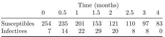
Time (months)

0 0.5 1 1.5 2 2.5 3 4

Susceptibles 254 235 201 153 121 110 97 83 Infectives 7 14 22 29 20 8 8 0

Table 4: Eyam plague data.

5.3.2 Pseudo-marginal Metropolis-Hastings

Let y = {yti}, i = 1, . . . ,8 denote the observations at times 0 = t1 < . . . < t8 = 4. The latent

Markov jump process over the time interval (ti, ti+1] is denoted byX(ti,ti+1]={Xs|ti< s≤ti+1}.

Under the assumption of no measurement error, we have that Xti = yti, i = 1, . . . ,8. Upon

ascribing a prior density p(c) to the rate constants c, Bayesian inference may proceed via the marginal parameter posterior

p(c|y)∝p(c)p(y|c) (21)

where

p(y|c) =

7

Y

i=1

p(yti+1|yti, c) (22)

is the observed data likelihood. Although p(y|c) is intractable, we note that each term in (22) can be seen as the normalising constant of

p(x_(ti,ti+1]|xti, yti+1, c)∝p(yti+1|xti+1)p(x(ti,ti+1]|xti, c)

wherep(yti+1|xti+1) takes the value 1 ifxti+1 =yti+1 and 0 otherwise. Hence, running steps 1(a) and

(b) of Algorithm 2 withx0 andyT replaced byxti andyti+1 respectively, can be used to unbiasedly

estimate p(yti+1|yti, c). No resampling is required, since only those trajectories that coincide with

the observationyti+1 will have non-zero weight. By analogy with equation (4), and allowing explicit

dependence on cwe have the unbiased estimator

ˆ

p(yti+1|yti, c) =

1 N

N X

j=1

p(yti+1|X

j ti+1)

p(Xj_(t

i,ti+1]|xti, c) q(Xj_(t

i,ti+1]|xti, yti+1, c)

(23)

where Xj_(t

i,ti+1] is an independent draw from q(·|xti, yti+1, c). Then, multiplying the ˆp(yti+1|yti, c), i= 1, . . . ,7, gives an unbiased estimator of the observed data likelihood p(y|c).

An alternative unbiased estimator of the observed data likelihood can be found by using (a special case of) the alive particle filter (Del Moral et al., 2015). Essentially, forward draws are repeatedly generated from p(·|xti, c) (via Gillespie’s direct method) until N + 1 trajectories that

match the observation are obtained. Letni denote the number of simulations required to generate

N + 1 matches withyti+1. The estimator is then given by

ˆ

p(yti+1|yti, c) =

N ni−1

. (24)

LetU ∼p(·|c) denote the flattened vector of all random variables required to generate the esti-mator of observed data likelihood, which we denote by ˆpU(y|c). The pseudo-marginal

Metropolis-Hastings (PMMH) scheme is an MH scheme that targets the joint density

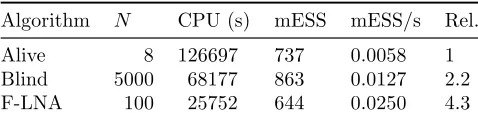
Algorithm N CPU (s) mESS mESS/s Rel.

Alive 8 126697 737 0.0058 1 Blind 5000 68177 863 0.0127 2.2 F-LNA 100 25752 644 0.0250 4.3

Table 5: SIR model. Number of particles N, CPU time (in seconds s), minimum ESS, minimum

ESS per second and relative (to Blind) minimum ESS per second. All results are based on 104

iterations of each scheme.

for which it is easily checked that

Z

p(c, u)du∝p(c)

Z

ˆ

pu(y|c)p(u|c)du

∝p(c)p(y|c)

where the last line follows from the unbiasedness property of ˆpU(y|c). Hence we see that the target

posterior p(c|y) is a marginal of the joint density p(c, u). Now, running an MH scheme with a proposal density of the formq(c∗|c)p(u∗|c∗) gives the acceptance probability

min

1,p(c ∗_)ˆp

u∗(y|c∗) p(c)ˆpu(y|c)

×q(c|c ∗₎

q(c∗_|c)

.

Practical advice for choosingN to balance mixing performance and computational cost can found

in Doucet et al. (2015) and Sherlock et al. (2015). The variance of the log-posterior (denoted σ_N2 ,

computed with N samples) at a central value of c (e.g. the estimated posterior median) should

be around 2. In what follows, we use a random walk on logc as the parameter proposal. The

innovation variance is taken to be the marginal posterior variance of logc estimated from a pilot run, and further scaled to give an acceptance rate of around 0.2–0.3. We followed Ho et al. (2018) by adopting independent N(0,1002_{) priors for logc}

i,i= 1,2.

Although we do not pursue it here, the case of non-zero measurement error is easily accom-modated by iteratively running Algorithm 2 in full, for each observation time ti,i= 1, . . . ,7. At

time ti, yT is replaced by yti+1 and x0 is replaced by x

j

ti. At time t1, x0 can be replaced by a

draw from a prior densityp(xt1) placed on the unobserved initial value. The product (across time)

of the average unnormalised weight can be shown to give an unbiased estimator of the observed data likelihood (Del Moral, 2004; Pitt et al., 2012). We refer the reader to Golightly and Wilkinson (2015) and the references therein for further details of the resulting Metropolis-Hastings scheme.

5.3.3 Results

We ran PMMH using the observed data likelihood estimator based on (23), with trajectories drawn either using forward simulation or the Fearnhead approach based on the LNA (without restart). We designate the former as “Blind” and the latter as “F-LNA”. Additionally, we ran PMMH using the observed data likelihood estimator based on (24). We designate this scheme as “Alive”.

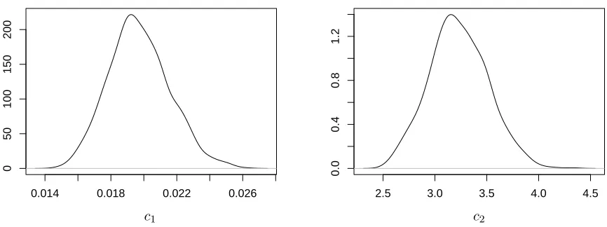
We ran each scheme for 104 _{iterations. For Alive, we followed Drovandi and McCutchan (2016)}

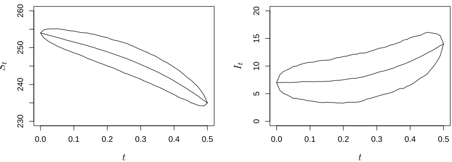
by terminating any likelihood calculation that exceeded 100,000 forward simulations, and rejecting the corresponding move. Marginal posterior densities can be found in Figure 4 and are consistent with the posterior summaries reported by Ho et al. (2018). Figure 5 summarises the posterior distribution ofXt|x0, y0.5, c, wherecis fixed at the estimated posterior mean. We note the

minimum (over each parameter chain) effective sample size per second (mESS/s). As is appropriate for MCMC output, we use

ESS = niters

1 + 2P∞_k=1αk

whereαk is the autocorrelation function for the series at lagkandnitersis the number of iterations

in the main monitoring run. Inspection of Table 5 reveals that although use of the alive particle filter

only requires N = 8 (compared to N = 5000 and N = 100 for Blind and F-LNA respectively), it

exhibits the largest CPU time. We found that for parameter values in the tails of the posterior, Alive

would often require many thousands of forward simulations to obtainN = 8 matches. Consequently

Alive is outperformed by Blind by a factor of 2 in terms of overall efficiency. Use of the LNA-driven bridge (without restart) gives a further improvement over Blind of a factor of 2.

6

Discussion

Performing efficient sampling of a Markov jump process (MJP) between a known value and a poten-tially partial or noisy observation is a key requirement of simulation-based approaches to parameter inference. Generating end-point conditioned trajectories, known as bridges, is challenging due to the intractability of the probability function governing the conditioned process. Approximating the hazard function associated with the conditioned process (that is, the conditioned hazard), and cor-recting draws obtained via this hazard function using weighted resampling or Markov chain Monte Carlo offers a viable solution to the problem. Recent approaches in this direction (Fearnhead, 2008; Golightly and Wilkinson, 2015) give approximate hazard functions that utilise a Gaussian approximation of the MJP. For example, Golightly and Wilkinson (2015) approximates the num-ber of reactions between observation times as Gaussian. Fearnhead (2008) recognises that the conditioned hazard can be written in terms of the intractable transition probability associated with the MJP. The transition probability is replaced with a Gaussian transition density obtained from the Euler-Maruyama approximation of the chemical Langevin equation. In both approaches the remaining time until the next observation is treated as a single discretisation. Consequently, the accuracy of the resulting bridges deteriorates as the inter-observation time increases.

Starting with the form of the conditioned hazard function, we have proposed a novel bridge con-struct by replacing the intractable MJP transition probability with the transition density governing the linear noise approximation (LNA). Whilst our approach also involves a Gaussian approxima-tion, we find that the tractability of the LNA can be exploited to give an accurate bridge construct. Essentially, the LNA solution can be re-integrated over each observation window to maintain accu-racy. The cost of ‘restarting’ the LNA in this way is likely to preclude its practical use. We have therefore further proposed an implementation that only requires a single full integration of the ordinary differential equation system governing the LNA. Our experiments demonstrated superior performance of the LNA based bridge over existing constructs, especially in data-sparse scenar-ios. Whilst the LNA is known to give a poor approximation of the MJP in low count scenarios (Schnoerr et al., 2017), we note that its role here is in the approximation of transition densities over ever diminishing time intervals. Moreover, the resulting approximate conditioned hazard function is corrected for via a weighted resampling scheme. Consequently, we find that use of the LNA in this way is relatively robust to situations involving low counts. Using a real data application, we further demonstrated the potential of the proposed methodology in allowing efficient parameter inference.

method to an infinite statespace pseudo-marginal MCMC algorithm which uses random truncation (e.g. Glynn and Rhee, 2014) to produce a realisation from an unbiased estimator of the likelihood when the observations are exact. In contrast to the algorithms which we have investigated, which simulate paths for the process and whose performance improves as the observation noise increases, any extension to the algorithm of Georgoulas et al. (2017) that allows for observation error would reduce the efficiency of the algorithm. This suggestes the possibility that for small enough ob-servation noise an extension to the algorithm in Georgoulas et al. (2017) might be more efficient than our non-restarting bridge. Investigations in to the relative efficiencies of such algorithms are ongoing.

This article has focused on bridges from a known initial condition. When the initial condition is unknown, such as typically arises in a particle filter-based analysis, a sample from the distribution of the initial state, {x1

0, . . . , xN0 }, is available and a separate bridge to the observation is required

from each element of the sample. In this case, two different implementations of the LNA bridge without restarting are possible. In the first implementation, trajectories Xi|xi₀, yT are generated

using one full integration of (11), (13) and (14) over (0, T]for each xi₀. That is, each trajectory has (11) initialised at xi

0. In the second implementation, (11), (13) and (14) are integrated just once,

irrespective of the number of required trajectories. This can be achieved by initialising (11) at some

plausible value e.g. E(X0). Although the second implementation will be more computationally

efficient than the first, some loss of accuracy is expected, especially when the uncertainty in X0 is

large. A single integral, however, may well be adequate in the cases which are the focus of this article: where the observation noise is small. Investigating the efficiency of the bridge construct in this scenario, as well as in multi-scale settings (see e.g. Thomas et al., 2014) where some reactions regularly occur more frequently than others, remains the subject of ongoing research.

References

Bailey, N. T. J. (1964).The elements of stochastic processes with applications to the natural sciences. Wiley, New York.

Bladt, M., Finch, S., and Sørensen (2016). Simulation of multivariate diffusion bridges. Journal of the Royal Statistical Society Series B: Statistical Methodology, 78:343–369.

Bladt, M. and Sørensen (2014). Simple simulation of diffusion bridges with application to likelihood inference for diffusions. Bernoulli, 20:645–675.

Boys, R. J., Wilkinson, D. J., and Kirkwood, T. B. L. (2008). Bayesian inference for a discretely observed stochastic kinetic model. Statistics and Computing, 18:125–135.

Br´emaud, P. (1981). Point Processes and Queues: Martingale Dynamics. Springer Verlag, New

York.

Cox, J. C., Ingersoll, J. E., and Ross, S. A. (1985). A theory of the term structure of interest rates.

Econometrica, 53:385–407.

Del Moral, P. (2004). Feynman-Kac Formulae: Genealogical and Interacting Particle Systems with

Applications. Springer, New York.

Del Moral, P., Jasra, A., Lee, A., Yau, C., and Zhang, X. (2015). The alive particle filter and its use in particle Markov chain Monte Carlo. Stochastic Analysis and Applications, 33:943–974.

Doucet, A., Pitt, M. K., and Kohn, R. (2015). Efficient implementation of Markov chain Monte Carlo when using an unbiased likelihood estimator. Biometrika, 102:295–313.

Drovandi, C. C. and McCutchan, R. (2016). Alive SMC2: Bayesian model selction for low-count

time series models with intractable likelihoods. Biometrics, 72:344–353.

Drovandi, C. C., Pettitt, A. N., and McCutchan, R. (2016). Exact and approximate Bayesian inference for low count time series models with intractable likelihoods.Bayesian Analysis, 11:325– 352.

Elf, J. and Ehrenberg, M. (2003). Fast evolution of fluctuations in biochemical networks with the

linear noise approximation. Genome Research, 13(11):2475–2484.

Fearnhead, P. (2008). Computational methods for complex stochastic systems: a review of some

alternatives to MCMC. Statistics and Computing, 18:151–171.

Fearnhead, P., Giagos, V., and Sherlock, C. (2014). Inference for reaction networks using the Linear Noise Approximation. Biometrics, 70:457–456.

Fuchs, C. (2013). Inference for diffusion processes with applications in Life Sciences. Springer, Heidelberg.

Georgoulas, A., Hillston, J., and Sanguinetti, G. (2017). Unbiased Bayesian inference for population

Markov jump processes via random truncations. Statistics and Computing, 27:991–1002.

Gillespie, D. T. (1977). Exact stochastic simulation of coupled chemical reactions. Journal of

Physical Chemistry, 81:2340–2361.

Gillespie, D. T. (1992). A rigorous derivation of the chemical master equation. Physica A, 188:404– 425.

Gillespie, D. T. (2000). The chemical Langevin equation. Journal of Chemical Physics, 113(1):297– 306.

Glynn, P. W. and Rhee, C.-H. (2014). Exact estimation for markov chain equilibrium expectations.

J. Appl. Probab., 51A:377–389.

Golightly, A. and Kypraios, T. (2017). Efficient SMC2 schemes for stochastic kinetic models.

Statistics and Computing. https://doi.org/10.1007/s11222-017-9789-8.

Golightly, A. and Wilkinson, D. J. (2015). Bayesian inference for Markov jump processes with

informative observations. SAGMB, 14(2):169–188.

Ho, L. S. T., Xu, J., Crawford, F. W., Minin, V. N., and Suchard, M. A. (2018). Birth/birth-death processes and their computable transition probabilities with biological applications. Journal of Mathematical Biology, 76(4):911–944.

Komorowski, M., Finkenstadt, B., Harper, C., and Rand, D. (2009). Bayesian inference of biochem-ical kinetic parameters using the linear noise approximation. BMC Bioinformatics, 10(1):343.

Kurtz, T. G. (1970). Solutions of ordinary differential equations as limits of pure jump markov processes. J. Appl. Probab.., 7:49–58.

Lin, J. and Ludkovski, M. (2013). Sequential Bayesian inference in hidden Markov stochastic kinetic models with application to detection and response to seasonal epidemics. Statistics and Computing, 24:1047–1062.

Matis, J. H., Kiffe, T. R., Matis, T. I., and Stevenson, D. E. (2007). Stochastic modeling of aphid

population growth with nonlinear power-law dynamics. Mathematical Biosciences, 208:469–494.

McKinley, T. J., Ross, J. V., Deardon, R., and Cook, A. R. (2014). Simulation-based Bayesian inference for epidemic models. Computational Statistics and Data Analysis, 71:434–447.

Petzold, L. (1983). Automatic selection of methods for solving stiff and non-stiff systems of ordinary differential equations. SIAM Journal on Scientific and Statistical Computing, 4(1):136–148.

Pitt, M. K., dos Santos Silva, R., Giordani, P., and Kohn, R. (2012). On some properties of

Markov chain Monte Carlo simulation methods based on the particle filter. J. Econometrics,

171(2):134–151.

Raggett, G. (1982). A stochastic model of the Eyam plague. Journal of Applied Statistics, 9:212– 225.

Rao, V. and Teh, Y. W. (2013). Fast MCMC sampling for Markov jump processes and extensions.

Journal of Machine Learning Research, 14:3295–3320.

Ruttor, A. and Opper, M. (2009). Efficient statistical inference for stochastic reaction processes.

Physical review letters, 103:230601.

Ruttor, A., Sanguinetti, G., and Opper, M. (2010). Approximate inference for stochastic reaction networks. In Lawrence, N. D., Girolami, M., Rattray, M., and Sanguinetti, G., editors, Learning and Inference in Computational Systems Biology, pages 277–296. The MIT press.

Schauer, M., van der Meulen, F., and van Zanten, H. (2017). Guided proposals for simulating multi-dimensional diffusion bridges. Bernoulli.

Schnoerr, D., Sanguinetti, G., and Grima, R. (2017). Approximation and inference methods for stochastic biochemical kinetics - a tutorial review. Journal of Physics A, 50:093001.

Sherlock, C., Golightly, A., and Gillespie, C. S. (2014). Bayesian inference for hybrid discrete-continuous systems biology models. Inverse Problems, 30:114005.

Sherlock, C., Thiery, A., Roberts, G. O., and Rosenthal, J. S. (2015). On the effciency of pseudo-marginal random walk Metropolis algorithms. The Annals of Statistics, 43(1):238–275.

Sidje, R. B. and Stewart, W. J. (1999). A numerical study of large sparse matrix exponentials arising in Markov chains. Computational Statistics and Data Analysis, 29(3):345 – 368.

Stathopoulos, V. and Girolami, M. A. (2013). Markov chain Monte Carlo inference for Markov jump processes via the linear noise approximation. Philosophical Transactions of the Royal Society A, 371:20110541.

Thomas, P., Popovic, N., and Grima, R. (2014). Phenotypic switching in gene regulatory networks.

PNAS, 111:6994–6999.

Whitaker, G. A., Golightly, A., Boys, R. J., and Sherlock, C. (2017). Improved bridge constructs for stochastic differential equations. Statistics and Computing, 27:885–900.

0 1000 2000 3000 4000 5000

1 2 3 4

0 1000 2000 3000 4000 5000

1 2 3 4

0 1000 2000 3000 4000 5000

1 2 3 4

P S fr ag re p la ce m en ts

yT,(1) yT,(50) yT,(99)

T T T E S S E S S E S S lo g 1 0 (E S S /s ) lo g 1 0 (C P U ) 0 1 2 3 4

1 2 3 4

0

1

2

3

4

1 2 3 4

0

1

2

3

4

1 2 3 4

P S fr ag re p la ce m en ts y T , (1 ) y T , (5 0 ) y T , (9 9 ) T T T E S S lo g 1 0 (E S S /s ) lo

g10

(C

P

U

)

lo

g10

(C

P

U

)

lo

g10

(C P U ) −2 −1 0 1 2 3

1 2 3 4

−2 −1 0 1 2 3

1 2 3 4

−2 −1 0 1 2 3

1 2 3 4

P S fr ag re p la ce m en ts y T , (1 ) y T , (5 0 ) y T , (9 9 ) T T T E S S lo

g10

(E S S /s ) lo

g10

(E S S /s ) lo

g10

(E S S /s ) lo g 1 0 (C P U )

Figure 2: Lotka-Volterra model. Effective sample size (ESS, top row), log (base 10) computing time in seconds (CPU, middle row) and log (base 10) effective sample size per second (ESS/s,

bottom row) based on the output of the weighted resampling algorithm withN = 5000 and yT ∈

0

1000

2000

3000

4000

5000

1 2 3 3

1.0

1.5

2.0

2.5

1 2 3 4

1.0

1.5

2.0

2.5

1 2 3 4

P

S

fr

ag

re

p

la

ce

m

en

ts

T T

T

E

S

S

lo

g10

(E

S

S

/s

)

lo

g10

(C

P

U

)

Figure 3: Lotka-Volterra model. (a) Effective sample size (ESS, left panel), log (base 10) computing time in seconds (CPU, middle panel) and log (base 10) effective sample size per second (ESS/s, right panel) based on the output of the weighted resampling algorithm withN = 5000 andyT =yT,(50),

T = 1,2,3,4. Dotted lines: x0 = (10,10)′ and σ = 1. Dashed lines: x0 = (25,25)′ and σ = 2.5.

Solid lines: x0 = (50,50)′ and σ = 5.

0.014 0.018 0.022 0.026

0

50

100

150

200

2.5 3.0 3.5 4.0 4.5

0.0

0.4

0.8

1.2

P

S

fr

ag

re

p

la

ce

m

en

ts

c1 c2

0.0 0.1 0.2 0.3 0.4 0.5

230

240

250

260

0.0 0.1 0.2 0.3 0.4 0.5

0

5

10

15

20

P

S

fr

ag

re

p

la

ce

m

en

ts

It St

t t