Operator Equation and Application of Variation Iterative Method

(1)

Operator Equation and Application of Variation

Iterative Method

Ning Chen, Jiqian Chen

School of Science, Southwest University of Science and Technology, Mianyang, China Email: [email protected]

Received June 8,2012; revised July 8, 2012; accepted July 15, 2012

ABSTRACT

In this paper, we study some semi-closed 1-set-contractive operators A and investigate the boundary conditions under which the topological degrees of 1-set contractive fields, deg



I A, ,p



are equal to 1. Correspondingly, we can

obtain some new fixed point theorems for 1-set-contractive operators which extend and improve many famous theorems such as the Leray-Schauder theorem, and operator equation, etc. Lemma 2.1 generalizes the famous theorem. The cal- culation of topological degrees and index are important things, which combine the existence of solution of for integra- tion and differential equation and or approximation by iteration technique. So, we apply the effective modification of He’s variation iteration method to solve some nonlinear and linear equations are proceed to examine some a class of integral-differential equations, to illustrate the effectiveness and convenience of this method.

Keywords: Topology Degrees and Index; 1-Set-Contract Operators; Modified Variation Iteration Method; Integral-Differential Equation

1. Introduction

In recent years, the fixed point theory and application has rapidly development.

That topological degree theory and fixed point index theory play an important role in the study of fixed points for various classes of nonlinear operators in Banach spaces (see [1-6]). We begin recall theorem A and lemma 1.1 [3]. Then, several new fixed point theorems are obtained in Section 2, and the common solutions of the system of operator equations in Section 3. We also extend some examples for search solution of integral equation and integral-differential equation in Section 4 and Sec-tion 5 by variaSec-tion iterative method. In last part, we com- pare some figures, by numerical test and note that simple case of Schrodinger equation. The main results are Theo-rem 2.2, TheoTheo-rem 3.4-3.5, Example 3, Example 6, etc.

2. Several Fixed Point Theorems

Let be a real Banach space, a bounded open subset of and

E 

E  the zero element of E.

If A: E is a completely continuous operator, we

have some well known theorems as follows (see [3,4]). First, we need following some definitions and conclusion (see [3]). For convenience, we first recall theorem A.

Theorem A (see Theorem 1.1 in [3]) Suppose that A

has no fixed point on and one of the following

conditions is satisfied,

,



1) (Leray-Schauder) ,Axx, for and  1; 2) (Rothe) Ax  x , for all x;

3) (Petryshyn) Let  , Ax  Axx , for all ;

x

4) (Altman) Axx2 Ax2 x2, for all x.

then deg



I A, ,



1, and hence A has at least one

fixed point in .

Lemma 2.1 (see Corollary 2.1 [3]) Let be a real Banach Space,

E

 is a bounded open subset of E and .



IfA: Eis a semi-closed 1-set-contractive opera-

tor such that satisfies the L-S boundary condition ,

Axtx for all x and t1, (2.1)

then deg



I A, ,



1, and so A has a fixed point

in .

Remark This lemma 2.1 generalizes the famous L-S theorem to the case of semi-closed 1-set-contractive operators.

First, we state following some extend conclusion (see theorem [5]).

Theorem 2.2 Let , ,E  A be the same as in lemma 2.1. Moreover, if there exists  1,0, 0 , - positive integer such that

n

( ) ( )

4 2 ,

for all .

n n n n

Ax x     Ax x   Ax  x    

 (2.2)

(2)

Then deg



I A, ,



1 if A has no fixed points

on  and so A has a fixed point in .

Proof.By lemma 2.1, we can prove theorem 2.2. Sup-pose that A has no fixed point on .

Then assume it is not true, there exists x0,01

such that Ax00 0x . It is easy to see that 01.

Now, consider the function defined by

  



( )





( )

4 n 2n

f t  t      t     1,

1

, for any t1.

Since

  











( )

( ) 1

4

2 0

n

f t n n t

n n t

                           

and by formal differential, f t

 

is a strictly increasing

function in



1,



, and so f t

 

 f

 

1 for . Thus

1 t





( )





( )





4 2 1 2

for any 1.

n n n n

t t t

t                   1, t 

Consequently, noting that x0 0,  0 1, we have





( ) ( )

0 0 0 0 0

( ) ( )

0

( )

0 0 0 0

4 4 2 1 2 , n n n n

n n n

Ax x x x

x

Ax x Ax x

                                _   _    )   

which contradicts (2.2), and so the condition (LS is

satisfied. Therefore, it follows from lemma 2.1 that the conclusions of theorem 2.2 hold.

Theorem 2.3 Let be the same as in lemma 2.1. Moreover, if there exists

, , E  A

1, 0, 0

     ,

positive integer such that

,

m n





( )

1

, for all .

n n n

n

Ax m x Ax mx Ax

x x                  

  (2.3)

Then deg



I A, ,



1, if A has no fixed points

on  and so A has a fixed point in .

Proof.Similar proof of that theorem 2.2. Now, we consider the function defined by

  



( )





( )

1n n 1

f t   t m      t m      , for any t1, and f

 

t 0.

So,

 

f t is a strictly increasing function in



1,



, and

 

1

f t  f for t1. We have  













( ) ( ) 1 1 1, n n n n

t m t m

t m t

                   

for any t1.

Consequently, noting that x0 0, 01, we have





( )

0 0 0 0

( )

0

1 n n n

n

Ax m x Ax mx Ax

x    0                

which contradicts (2.3). Therefore, it follows from lemma 2.1 that the conclusions of theorem 2.3 hold.

Corollary 2.4 If





( )

1 n n ,

Ax m x      Axmx   Axn (2.4)

then (2.3) holds. By theorem 2.3, A has a fixed point in

.

We get easy theorem 2.5 in bellow. So, extend (vi) of theorem 2.6 in [3], omit the similar proof.

Theorem 2.5 Let E, , A be the same as in lemma

2.1. Moreover, if there exists  1,1 and - positive integer such that

,

m n

( )

,for all .

n n n

Ax  Axmx  x   x (2.5) Then deg



I A, ,



1, if A has no fixed points

on  and so A has at least one fixed point in .

(Let m1, that is theorem 2.4 in [5]).

3. Operator Equations

We will extend Lemma 2 and Theorem 2, adopt same notation and method in [7]in following form.

Let be a real Banach space, and -positive integer.

E p1,m

Lemma 3.1 When t1,p1 the following holds:



1



1



mp 1 mp



1



mp

m t  t  t .

Proof.Let

 

mp 1



1



1



mp



1



mp

f t mt   m t  t , similar the proof of lemma 2 in [7], we easy get

 

0.

f t  In fact, by derivative of it, we have

 



 

















1 1 1 1 1 1 1 1 1 ,

1 1 1

mp mp

mp

mp mp

mp

f t m mp t m mp t

mp t

mp t m t t

             .    _      _ Since























1 1 1 1 1 1 1 1 1 1 1 1

1 1 1

1 ₁ 1 1 ₁ 1

1 1 1 1

2 0. 1 mp mp mp mp mp mp mp t t m t t t

m t t

m t m t

m             _ _ _ _ _    _ _ _ _ _ _ _            _  _  _  _            

(3)





1







1 ₁ mp ₁ mp

mp

t   t   m t1 1,

0 that is,







1





1

1 ₁ ₁ mp ₁ mp

mp

mp t_   m t   t _ .

Thus, f

 

t 0 Therefore, f t

 

0, is a strictly mo-

notone increasing function in



.When we

have and



1

t

 

1 ,

f t  f _f

 

1  _m 2mp0, _{that is}

.

 

f t 0

Hence,











1

1 mp 1 1mp

mp

t  t  m t  1,

where We complete the proof of this lemma 3.1.

1, 1.

t p

Theorem 3.2 Let be a bounded open convex subset in and

D

;

D

,

E  Suppose that A D: E is a

semi-closed 1-set-contradictive operator, and m, n -posi-tive integer such that



1



mp mp mp mp

m Axx  Axx  Ax  x ,

. for every

, 1

xD p (3.1)

Then the operator equation Axx has solution

in .

a

D

Proof. By (3.1), we know that Axx has no

solu-tion in D, that is xAx, for every xD. We shall

prove ,

xtAx for every t

 

0,1 , for every xD. (3.2)

In fact, suppose that (3.2) is not true that is there exists a t₀

 

0,1 ,and an x₀D such that x₀t Ax₀ ₀, that

is 1

0 0 0

Ax tx .

By (3.1), we obtain





1 1

0 0 0 0 0

4 1

0 0 0

1

,

mp mp

mp

m t x x t x x

t x x

 



   

 

for every ₀ This is because

, 1

x D p .

0 ;

x D hence x₀ 0, then we

have







1

 

1



0 0 0

1 1 1 mp mp

m t   t t 

1



1.

,

mp

 

Let 0 as we have

That is





then this

is a contradiction to Lemma 3.1. ,

tt t0

 

0,1 ,





1 1mp

m t 

1. t



1



mp

t



1 mp

t

 

Thus, ,

xtAx for every t

 

0,1 , for everyxD. (3.3) From (3.2) and (3.3), we know that xtAx. By Ref [6], we obtain that i A D E



, ,



1. Then this operator equation Axx has a solution in D.

Theorem 3.4 Let be a bounded open convex subset in and

D ; D ,

E   Suppose that , :A B DE are

semi-closed.

1-set-contradictive operator, and m, n-positive integer such that



1



, for every , 1.

mp mp mp

mp

m Ax x Ax x Ax

Ax Bx x D p

    

    (3.4)

Then the operator equation Axx Bx, x has common solution in (omit the proof of this theorem).

a

D

Theorem 3.5 Let Same as assume theorem 3.1. Sup- pose that , , :A B C DE are semi-closed 1-set-contradictive operator, and m, n-positive integer, substitute (3.5) for inequality bellow



1



, , 1.

mp mp mp

mp

m Ax x Ax x Ax

Ax Bx Cx x D p

    

    

Then the operator equation Axx Bx Cx,  x has common solution in (omit this proof).

a D

4. Solution of Integral Equation

Recently, the variational iteration method (VIM) has been favorably applied to some various kinds of nonlinear problems, for example, fractional differential equations, nonlinear differential equations, nonlinear thermo- elasticity, nonlinear wave equations.

In this section, we apply the variation iteration method (simple writing VIM) to Integral equations bellow (see [8,9]). To illustrate the basic idea of the method, we con-sider:

 



.

L u t_ _N u t_ _g t



The basic character of the method is to construct func-tional for the system, which reads:

 

1 ₀ d

x

n n n n

u x u x 



 s Lu Lu Nu g s  s

Which can be identified optimally via variation theory, is the nth approximate solution, and

n

u un denotes a

restricted variation, i.e.,  un 0. There is a iterative

formula:

 

   

1 , d

b

n _a n

u x  f x 



k x t u t t,

d of this equation

 

b

   

,

a

u x  f x 



k x t u t t (*) Theorem 4.1 (see theorem 3.1 [8]) Consider the iteration scheme u0

 

x  f x

 

,and

 

   

1 , d

b

n _a n

u x  f x 



k x t u t t.

Now, for n0,1, 2, , to construct a sequence of successive iterations that for the for solution of integral equation (*).



n

 

(4)

In addition, we assume that

 

2 _{, d d} 2 _, b b

a ak x t x tB  

 

and

 

2_{ } then if , ,

a b

f x L  1 ,B the above iteration

converges in the norm of to the solution of integral equation (*).  

2 ,

a b L

Corollary 4.2 If k x t

 

, k x t1

 

, k2

 

x t, , and

 

2 _{, d d} 2 _,

b b

a ak x t x tB  

 

then assume

 

2_{ } if , ,

a b

f x L  1 ,B the above iter-

ation converges in the norm of to the solution of integral equation (*).  

2 ,

a b L

Example 1 Consider that integral equation

 

1

   

0 d

u x xx x 



xt u t t (4.1)

where u(0)0, and

 





0 0 1,0

u x xxx     1

n

From that

 

1

   

1

0 d .

n

u x xx  x 



xt u_ t t

We have 1 1

2 2

l

 

 

  

 _ _ 

 

1 3

0

 

1

   

1 ₀ d

,

u x x x x xt u t t

x x x xl

 

 

   



 

1

   

2 ₀ d

1 .

3

u x x x x xt u t t

x x x lx

 

  

   

 

    _  _

 



1

From theorem 4.1 and simple computation, we obtain again that

 

2 1 1

 

2 2

0 0

1

d d d d ,

9

b b

a a xt x t xt x t B

 

 

and by theorem 4.1 if  3, then iterative

 

1

   

1 ₀ d

n

u _ x xx x 



xt u_n t t

is convergent.

Then inductively, we have

 

1

   

1 ₀

2

d

1

3 3 3

n

u x x x x xt u t t

x x x

lx

 



  



    

  

 _{   } _{ }

        

     

 

 



 .

n

 

The solution of integral Equation (4.1) by calculating as follows.

 



 





₁ 1







1

lim

2 2 3 3 3

n n

u x u x x x x

x

 

.

   





 

   

     

Example 2 We consider that integral equation

 

₄ 1



  

0 d ,

u x xx 



xtt u t t (4.2)

 

4





0 0 1

u x xx   . From (*), we have that

 

₄ 1



  

1 ₀ d

n n

u x xx 



xtt u t t

In fact,

1 1

2 2

0 0 2

( , ) d ( ) d d 1 1 1 7

9 3 3 9

b b

a ak x t Ex t xt t x t

B

 

      

 

and by Corollary 4.2, then if  3 7 , iterative sequence is convergent the solution of Equation (4.2).

5. Some Effective Modification

In this section, we apply the effective modification method of He’s VIM to solve some integral-differential equa-tions.

In [10] by the variation iteration method (VIM) simu- late the system of this form

 

.

LuRuNug x

To illustrate its basic idea of the method .we consider the following general nonlinear system

 

, LuRuNug x

Lu the highest derivative and is assumed easily in-vertible, is a linear differential operator of order less than represents the nonlinear terms, and

R

,

L N g is the

source term. Applying the inverse operator 1

x

L to both

sides of Equation (1), and we obtain

 

1 1 _.

x x

u f L Ru L Nu

The variation iteration method (VIM) proposed by Ji-Huan He (see [5,10] has recently been intensively studied by scientists and engineers. the references cited therein) is one of the methods which have received much concern .It is based on the Lagrange multiplier and it merits of simplicity and easy execution. Unlike the tradi-tional numerical methods. Along the direction and tech-nique in [5], we may get more examples bellow.

Example 3 Consider the following integral-differential equation

 

1

 

(5)

0 4

d , 3

x

(5)

where In similar example1, we easy have it.

 

0 1, 0 2, 0 1, 0 1 u  u  u  u  .

According to the method, we divide f into two parts

defined by

 

_{ }

0 0 0

6 6

1

, ,

4 1 _.

3 6! 540

x x

f x x e u x f x x e

f x x x

    

   

Taking_{f x}

 

 _x _ex



_{1 540}



_x6_{, then we have}

 





₆ ₁



1

 



1 1 540 ₀ 0 d

,

x

x x

u x x e x L xtf t t

x e



   

 



where and the

proc-esses:

1

0 0 0 0 0

( ) x x x x x( )d d d d d ,

x

L  

    

 t t t t t

 





₆ ₁



1

 



1 1 540 ₀ d , 1.

x

n x n

u_ x   x e x L



xtu t t n

Thus, 1

 

, x n

u _ x  x e then u x

 

 x ex is the

exact solution of (5.1) by only one iteration leads to a solution.

Example 4 (similar example 3 in [5]) Consider the following nonlinear Fredholm integral equation

 

_{ }





1 1

2 2

0 0

1

2 0

9π 3 2

d

12 3 2

1

d .

3

1 ( ) 3

u x x t

u t u t

t

u t

   

 

 

 _ _

  



(5.2)

where from that arctan1π4, arctan 3π 3.

 





0 0 , 1 3π 4 , 0 ,

u x  f x x f x   f  f f₁

by iterative method:

 

_{ }

 





1 1

1 0 2 0 2

1

2 0

9π 3 2

d

12 3 2

1

, 1. 3

1 3

n

n n

n

u x x t

u t u t

t

d x n

u t

    _  _

 

 _ _

  





Clearly, u(x)x is evident exact solution of (5.2).

6. Some Notes for Schrodinger Equations

The quantum mechanics theory and application in more field are widely important meaning.

Along the direction and technique in [11] and [12], we may get more examples.

As we all know the solution of initial problem for Schrodinger equation bellow

 

2 _{, ,} _, _0,

,0 , .

n t

n

u ia u f x t x R t

u x  x x R

     

 

 

 (6.1)

Assume that real part and imaginary part of

   

x ,f x t, ,

 are real analytical function for n, xR then this solution of the problem may express in form:

 

2

_

_{ }

_

_

_{ }

_

0 0

,

, d !

k

t k

k k k

x k

u x t

ia

t x t f x

k    .







 

_

   (*)

Now, the authors consider again one-dimension Sch- rodinger equation as application form:

 

   

0, ,

xx x f x x x R

     (6.3)

 

2m



 

_

f x E V

h

 _  x . (6.4) where look in (6.3), that 

 

x be the part in space for

wave function 

 

x t, 

E

, the in (6.4) be the poten-tial function h be arrange plank constant, be the practical mass, express energy.



V x



m

The Equation (6.3) for with extensive equation, by cal-culating and search the general solution that

 

x C1sin



x f x

 



C2cos



x f x

 



   (6.5)

So, by (6.3) and with power of (6.4), we consider that two case:

1) (see [13,14]) The infinite deep power trap

 

2 _{2 ,}



2 2_π ₂ 2



2_, _{0,1, 2, .} n

V x  x E  h m n n 

2) The shake Power

 

2 _{2 ,}



_0.5



_, _{0,1, 2, .} n

V x  x E  n h n 

We take parameters m  h  1,C1C21. Then

 

2 2 2 2 2 2 2

2 2

2 2 2

2 π π

2 1

2

π , 0,1, 2, .

2

m h x n x

f x n

m h

x

n n



 

2

    

 

 

_  _ 

 

 



Furthermore, from (6.5), we obtain analytic solution for 

 

x and 

 

x . So, we have that

 



 



 





2 2

2 ₂

sin π 0.5

cos π 0.5 , 0,1, .

x x n x

x n x n

  

   

(6.61)

 









2

sin 2 1

cos 2 1 , 0,1, 2, .

x x n x

x n x n

   

    

(6.62)

See Figures 1 and 2 below.

(6)

-2 -1.5 -1 -0.5 0 0.5 1 1.5 2 -2

[image:6.595.314.533.86.278.2]

0 2 4 6 8 10

Fig 1, En=(n*phi)2,m=h=w=1,n=0,1,2,3,4.

X

Ph

i(

x

)

Phi0 Phi1 Phi2 Phi3 Phi4 V=x2/2

Figure 1.The φ(x) is the space form of wave function φ(x.t) for (6.3) under action of shake V(x) = 0.5x2_{, by}_φ

0, φ1, ···, φ4

express for 0-level, 1-level,···, 4-level wave function respec-tively.

-2 -1.5 -1 -0.5 0 0.5 1 1.5 2

-2 -1 0 1 2 3 4 5 6

Fig 2 En=(n+0.5),m=h=w=1,n=0,1,2,3,4.

X

Ph

i(

x)

,V

(x

)

V=x2/2 Phi0 Phi1 Phi2 Phi3 Phi4

Figure 2. The ϕ(x) is the space form of wave functionϕ(x,t) for (6.3) under action of shake power V(x) = 0.5x2_{, by}_φ

0,

φ1, ···, φ4 express for 0-level, 1-level,···, 4-level wave

func-tion respectively.

In fact, according to the finite difference principle, a one-dimensional Schrodinger equation can be converted into a set of nodal liner equations expressed in a matrix equation after the space is divided into a series of dis-crete nodes with an equal interval. The matrix left divi-sion command offered in the MATLAB software can be used to derive the function approximation of each un-known nodal function.

7. Concluding Remarks

In this Letter, we consider operator equations and apply

-2 -1.5 -1 -0.5 0 0.5 1 1.5 2

-1 -0.5 0 0.5 1 1.5 2

X

Ph

i(

x)

,V

(x)

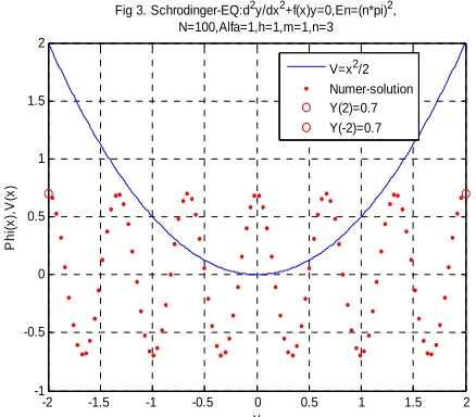
Fig 3. Schrodinger-EQ:d2y/dx2+f(x)y=0,En=(n*pi)2, N=100,Alfa=1,h=1,m=1,n=3

V=x2/2 Numer-solution Y(2)=0.7 Y(-2)=0.7

Figure 3. The φ(x) is numerical solution by action of (6.3) under the shake power V(x) = 0.5x2 _{and in boundary value}

condition φ(–2) = φ(2) = 0.7, the φ3(x) express 3-level (here

step length = 0.04, the energy En = ((nπ)2, n = 3).

-2 -1.5 -1 -0.5 0 0.5 1 1.5 2 -1

-0.5 0 0.5 1 1.5 2

X

Ph

i(

x

),

V(

x

[image:6.595.64.282.87.283.2]

)

Fig 4. Schrodinger-EQ:d2y/dx2+f(x)y=0,En=(n+0.5), N=100,Alfa=1,h=1,m=1,n=3

V=x2_/2 Numer-solution Y(2)=0.7 Y(-2)=0.7

Figure 4. The φ(x) is numerical solution by action of (6.3) under the shake power V(x) = 0.5x2_{and in boundary value}

condition φ(–2) = φ(2) = 0.7, the φ3(x) express 3-level (here

step length=0.04, the energy En = ((nπ)2, n = 3).

the variation iteration method to integral-differential equations, and extend some results in [3,8,10]. The obtained solution shows the method is also a very convenient and effective for various integral-differential equations, only one iteration leads to exact solutions. Recently, the im-pulsive differential delay equations is also a very inter-esting topic, and we may see [10]etc.

In our future work, we may try to do some research in this field and may be could obtain some better results.

8. Acknowledgements

[image:6.595.312.532.343.523.2] [image:6.595.64.282.348.534.2]

(7)

Founda-tion (No. 11ZB192) of Sichuan EducaFounda-tion Bureau and the key program of Science and Technology Foundation (No. 11ZD1007) of Southwest University of Science and Technology.

The author thanks the Editor kindest suggestions, and thanks the referee for his comments.

REFERENCES

[1] D. Guo and V. Lashmikantham, “Nonlinear Problems in abstract Cones,” Academic Press, Inc., Boston, New York, 1988.

[2] Y. J. Cui, F. Wang and Y. M. Zou, “Computation for the Fixed Index and Its Applications,” Nonlinear Analysis,

Vol. 71, No. 1-2, 2009, pp. 219-226.

doi:10.1016/j.na.2008.10.041

[3] S. Y. Xu, “New Fixed Point Theorems for 1-Set-Con- tractive Operators in Banach Spaces,” Nonlinear Analysis,

Vol. 67, No. 3, 2007, pp. 938-944.

doi:10.1016/j.na.2006.06.051

[4] N. Van Luong and N. X. Thuan, “Coupled Fixed Points in Partial Ordered Metric Spaces and Application,”

Nonlinear Analysis, Vol. 74, No. 3, 2011, pp. 983-992. doi:10.1016/j.na.2010.09.055

[5] N. Chen, and J. Q. Chen, “New Fixed Point Theorems for 1-Set-Contractive Operators in Banach Spaces,” Nonlin-ear Analysis, Vol. 6, No. 3, 2011, pp. 147-162.

[6] G. Z. Li, “The Fixed Point Index and the Fixed Point Theorems of 1-Set-Contrac-Tive Mappings,” Proceedings of the American Mathematical Society, Vol. 104, No. 4,

1988, pp. 1163-1170.

doi:10.1090/S0002-9939-1988-0969052-9

[7] C. X. Zhu and Z. B. Xu, “Inequality and Solution of an Operator Equation,” Applied Mathematics Letters, Vol. 21, No. 6, 2008, pp. 607-611.

doi:10.1016/j.aml.2007.07.013

[8] R. Saadati, M. Dehghan, S. M. Vaezpour and M. Saravi, “The Convergence of He’s Variational Iteration for Solv-ing Integral Equations,” Computers & Mathematics with Applications, Vol. 58, No. 11-12, 2009, pp. 2167-2171. doi:10.1016/j.camwa.2009.03.008

[9] Y. F. Xu, “The Variational Iteration Method for Autono-mous Ordinary Differential Equations with Fractional Order,” Journal of Hubei University Nationalities (Nature Science Edition), Vol. 29, No. 3, 2011, pp. 245-249.

[10] G. B. Asghar and S. N. Jafar, “An Effective Modification of He’s Variational Iteration Method,” Nonlinear Analy-sis: Real World Application, Vol. 10, No. 5, 2009, pp.

2828-2833. doi:10.1016/j.nonrwa.2008.08.008

[11] J. H. He, “Variational Iteration Approach to Schrodinger Equation,” Acta Mathematica Scienca, Vol. 21A, 2001,

pp. 577-583.

[12] S .Q. Wang and J. H. He, “Variational Iterative Method for Solving Integro-Differential Equations,” Physics Let-ters A, Vol. 367, No. 3, 2007, pp. 188-191.

doi:10.1016/j.physleta.2007.02.049

[13] Z. Z. Zhang and S. R. Lu, “Numerical Solution of Sch- rodinger Equation,” Journal of Shanxi Daton Universeity, Vol. 26, No. 2, 2010, pp. 22-24.

[14] Y. F. Wang and L. B. Tang, “Direct Solution of One-Di- mensional Schrodinger Equation through Finite Differ-ence and MATLAB Matrix Computation,” INFRARED