Generic scheduling in radar systems

(1)

Generic Scheduling

in Radar Systems

Appendices not included due to confidentiality

Author

Roelof Spijker

Supervisor UT

Johann Hurink

(2)

(3)

List of Figures

2.1 Doppler Radar Operation . . . 4

2.2 System Architecture . . . 7

2.3 Relation between operations . . . 8

2.4 Graph representation of earliest possible starting times. . . 9

2.5 Late event time graph . . . 10

2.6 Timeline partitioned by dummy jobs . . . 13

3.1 Resulting schedule for Example 3.1.1 . . . 16

3.2 Scheduling intervals . . . 17

3.3 System Architecture . . . 28

5.1 Fixing operations in graph representation . . . 34

5.2 Class Diagram . . . 38

6.1 Tracking scenario request sequences . . . 41

6.2 Rotating search radar coverage . . . 42

6.3 Search scenario result . . . 44

6.4 Search scenario running times per iteration . . . 45

6.5 Search scenario running times per iteration with local search (first fit) . . . 46

6.6 search scenario running times per iteration with shifting bottleneck 47 6.7 Tracking scenario result . . . 48

6.8 Tracking scenario running times per iteration . . . 48

6.9 Tracking scenario result after local search (first fit) . . . 49

6.10 Tracking scenario running times per iteration with local search (first fit) . . . 49

6.11 Tracking scenario result after local search (best fit) . . . 50

6.12 Tracking scenario running times per iteration with local search (best fit). . . 50

6.13 Tracking scenario result for shifting bottleneck heuristic . . . 51

6.14 Tracking scenario running times per iteration with shifting bot-tleneck heuristic . . . 51

(6)

(7)

List of Tables

3.1 Operation parameters for Example 3.1.1 . . . 16

6.1 Search scenario Job descriptions . . . 40

6.2 Tracking scenario Job descriptions . . . 41

A.1 Search scenario . . . 60

A.2 LRFoperations. . . 65

A.3 MRFoperations . . . 72

A.4 _SRFoperations. . . 79

A.5 _SURFoperations. . . 81

A.6 _FCoperations . . . 81

A.7 _TECHoperations . . . 81

B.2 _stingoperations . . . 83

(8)

(9)

Acknowledgements

(10)

(11)

Introduction

A scheduler decides how to assign resources to various tasks in order to optimize some objective. In our specific instance we want to allocate time to different tasks a radar system needs to perform. The decisions that need to be made are to select which tasks to process and to determine the order in which the selected tasks are processed. The intent is to create a generic scheduler. The scheduler should only have (or need) information about the essential aspects relevant to schedule the tasks, such as release time, processing time, priority, etc. Currently the schedulers designed at Thales are relatively specific to a certain project. There are project-specific scheduling rules in them, which makes it hard to port such a scheduler to a different system without having to redesign it. The aim of creating a generic scheduler is to be able to use it on multiple systems without the need to redesign it completely or in large parts.

This subject has already been researched during my internship[1]. The focus there was to show whether or not it is possible to use a more generic approach to solve the scheduling problem. The conclusion was that it is possible, but finding an optimal solution in the available amount of time is infeasible. Therefore the main question we try to answer in this report is whether we can find solutions of acceptable quality in a feasible amount of time.

(12)

(13)

Problem Description

In this chapter we introduce the problem. We begin with describing the problem with its background and then give a more formal mathematical description of the underlying scheduling problem.

2.1 Background

There are different kinds of radar systems with different responsibilities. In this report we consider shipborne radar systems with military applications. We can roughly divide this group into three smaller groups based on the tasks a radar system is designed to handle. First there are systems designed for surveilling a volume of space, called search radars. Second there are systems designed to accurately track one or more targets and guide projectiles, called tracking radars. Finally there are systems that combine these two tasks, called multi-function radars. All three of these types of systems use the same basic principle of reflected radio waves. However, there are different approaches to using this principle. We consider two different approaches, Frequency Modulation Contin-uous Wave (FMCW) and Doppler radar.

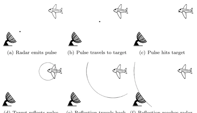
An FMCW radar continuously transmits radio waves with a frequency chang-ing over time defined by a predetermined pattern. A reflection of these radio waves implies the presence of an object. From the properties of this reflection, the shift in frequency due to the Doppler effect and the time passed between transmission and reception of the reflection, the radar system can determine the location, direction and speed of the object. To accurately detect objects a sweep is made over a certain frequency range which is then modulated by a certain known pattern and sent out over a period of time. We call such a sweep a burst.

(14)

(a) Radar emits pulse (b) Pulse travels to target (c) Pulse hits target

[image:14.595.164.486.127.312.2]

(d) Target reflects pulse (e) Reflection travels back (f) Reflection reaches radar

Figure 2.1: Doppler Radar Operation

pulses and listen for reflections. The antenna system processes the bursts and can only process one burst at a time. The tasks the radar system has to perform, like surveilling a volume of space, tracking a certain target or guiding a missile, all consist of one or more bursts for the antenna system to process. In order to complete the task all bursts that make up the task have to be processed. A radar system may have to perform many of these tasks in parallel. For instance we might want to search for new targets by sweeping 360 degrees around us, while keeping track of a number of targets we have found in the past and guiding a missile to a target we wish to engage. Since the antenna can only process one burst at a time we have to decide the order in which we process the bursts on the antenna and the exact moment at which we process each burst. The tasks to be performed are requested by a user, who can request more tasks than can be executed in the time available. Therefore we might also have to decide to reject certain requests.

(15)

still relevant. Finally the length of a burst often only becomes known shortly before it is transmitted. This is due to the fact that the burst length depends on parameters that have to be calculated and depend in turn on e.g. the position of the ship on the waves which is hard to predict. Since these true lengths only become known shortly before transmission they can not be taken into account when the decision on the bursts has to be made. However, we do have to deal with the consequences of the change in duration.

To some extent the above described problem is already being solved in every radar system, since these decisions need to be made in order for a radar system to operate. However, the problems that are actually being solved are special instances of the problem that are specific to the type of radar system they are solved in. This approach has as a drawback that the problem has to be solved again for each new radar system, keeping in mind its specific requirements. This increases the development time of new radar systems as well as increasing maintenance costs. Our aim is to design a generic method instead that solves the part of the problem that all types of radar systems have in common. If a specific system requires more or different functionality this part of the problem can be solved by an extra layer on top of the generic method. This limits the amount of work to be done to implementing the additional features and defining correct parameters for the generic method.

2.2 Problem Definition

The problem can be split up into two parts: the scheduling problem and the change in duration problem. The following subsections provide a short introduc-tion to the two problems, connecting the terms used in sketching the background to more familiar scheduling terms.

2.2.1 Scheduling Problem

(16)

2.2.2 Duration Change Problem

In Section2.1we stated that at the time of scheduling only expected processing times are known. Once the schedule is being executed the actual duration of each burst becomes known shortly before the scheduled transmission of the burst. Whether or not such a change leads to a direct problem depends on the nature of the change and the situation. Whenever the actual duration is shorter than the expected duration there is not directly a problem, the transmission is finished before the next burst is scheduled to start. If this is the case we might want to check if it is possible to start subsequent bursts earlier, since that leaves more room for possible changes in duration for these bursts. When the actual duration of a burst is longer than the expected duration and the longer duration causes the transmission of the burst to finish after the next burst is scheduled to start, we have a direct problem. The schedule has to be updated to accommodate these changes. This means subsequent bursts have to be delayed and/or rejected. When the actual duration of a burst is longer than the expected duration but the burst still finishes transmission before the next burst is scheduled to start, no action has to be taken.

We should take the subsequent nature of these problem into account when searching for a solution to the scheduling problem. It is of interest to develop methods to solve the scheduling problem which already take into account that the durations of bursts might change afterwards.

2.3 Problem Analysis

In this section we discuss the problems in more depth. We discuss the place of the scheduler in the radar system, look at the input we get from the system, what our output should look like and how we can compare different solutions. We start with some additional background information specifying the role and place of our problems in the system.

2.3.1 Place in the System

(17)

[image:17.595.97.442.99.224.2]

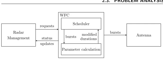
Radar Management WFC requests status updates Scheduler Parameter calculation bursts modified durations Antenna bursts

Figure 2.2: System Architecture

on time and sending the bursts to be transmitted to the antenna. Figure2.2

depicts a schematic overview of the system.

2.3.2 Scheduling Problem

In this subsection we discuss the scheduling problem in greater depth. We consider the input to the scheduling problem, discuss what makes up a solution and how these solutions can be compared. We also discuss the complexity of the scheduling problem.

Input

As we have seen in the previous subsection, the scheduler receives requests from a requester. In this subsection we explain how these requests are constructed and what information they contain. These requests together with the contained information constitute the input to the scheduling problem as defined in Section

2.2.1.

Each request is a request for a specific job to be executed. A job j in turn consists of a set ofnj operationsOj=

oj1, oj2, . . . , ojnj , which need to be ex-ecuted in this order. Furthermore, each job has a prioritypjwhich represents its

relative importance. These priorities are chosen from a finite set ofnP priorities

P ={p¯1,p¯2, . . . ,p¯nP}, such that ¯p1<p¯2< . . . <p¯nP. We denote Jk as the set of jobs withpj= ¯pk. Each operationohas a window [αo, βo] within which it has

to start.Furthermore, it has an expected processing timepoand a set ofn(o)

rela-tionsRo=

n

(or1, T

−

o,or1, T +

o,or1),(or2, T

−

o,or2, T +

o,or2), . . . ,(orn(o), T

−

o,o_rn

(o), T +

o,o_rn

(o))

o

,

where each relation is of the form or, To,o−r, T +

o,or

and denotes a relation be-tween the starting times of or and o respectively, stating there has to be a

minimum difference of To,o−r and a maximum difference of T +

o,or between the start oforando. Formally this is expressed by the constraints: sor+T

−

o,or ≤so andsor+T

+

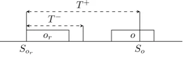
o,or ≥so, whereso denotes the starting time of operationo. Figure

2.3illustrates this relation.

Solution

(18)

Sor So

T− T+

[image:18.595.229.413.128.185.2]

or o

Figure 2.3: Relation between operations

and a starting time so for each operationo belonging to a jobj with Aj = 1.

We denote the set of jobs that are accepted by A with JA. That is to say,

JA={j ∈J|Aj = 1}. We denote a schedule as a tupleS = (A, s), wheres is

the set of starting times for the operations belonging to jobs inJA. The starting times in s have to define a unique ordering of the operations of the accepted jobs. On the other hand, for any given ordering of the operations there are in general infinitely many possible starting times. However, since we are mainly interested in schedules where the operations start as early as possible, we can restrict our attention to that schedule for a given ordering, where each operation starts as early as possible. If we can construct an efficient method to find the set of earliest possible starting times given a certain ordering of operations, we can uniquely define a schedule as a tupleS = (A, ~O), where O~ denotes an ordering of the operations of the jobs inJA_{. By confining ourselves to orderings instead}

of starting times, we can drastically limit the amount of possible solutions we have to consider, since there are infinitely many different sets of starting times, but onlyn! possible orderings of noperations.

In the following we show that finding the earliest possible starting times for a given ordered set of operations is equivalent to solving a longest path prob-lem. Finding longest paths can be accomplished efficiently (O(nm), where n

is the number of vertices and mthe number of edges) using the Bellman-Ford algorithm [2, 3]. Given an ordering O~ = (o1, o2, . . . , on) of n operations, we

consider a directed graph G on n+ 1 vertices. We introduce one vertexs as a starting vertex and n vertices corresponding to the n operations. Next we introduce arcs such that the length of the longest path fromsto a vertexoi

cor-responds to the earliest possible starting time of operationoiif all requirements

are met. The earliest possible starting time of an operationoi is influenced by

a number of constraints. First, the operation cannot start before the start of its window: soi ≥αoi. Second, the operation cannot start before the preced-ing operation has finished: soi ≥ soi−1 +poi−1. Third, the operation cannot start before T_o−

i,or time has expired since the start of a related operation or, i.e. for all or, To−i,or, T

+

oi,or

∈ Roi we have the constraint: soi ≥ sor+T

−

oi,or. Finally, the operation cannot start more than T+

oi,or after a related operation

or is set to start, i.e. for all or, To−i,or, T +

oi,or

∈ Roi we have the constraint:

soi ≤sor+T +

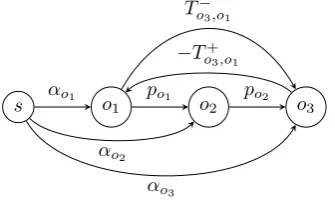
oi,or. The first constraint can be expressed by an arc from the start vertex sto vertexoi with weightαoi. The second constraint can be expressed by an arc from vertexoi−1 to vertexoi with weightpoi−1. The third constraint can be expressed by one arc from vertexor to vertexoiwith weightTo−i,or. The last constraint can be expressed by one arc from vertex oi to vertex or with

(19)

s o1 o2 o3 −T+

o3,o1

po2

po1

T_o−₃_,o₁

αo1

αo2

[image:19.595.186.354.129.229.2]

αo3

Figure 2.4: Graph representation of earliest possible starting times

Example 2.3.1 We have a single job j with 3 operations o1, o2 and o3. Furthermore, there is a maximum and a minimum relation between operations

o1 ando3. Figure2.4shows the graph corresponding to the example.

If we calculate now in the resulting graph the longest pathloi fromsto all other verticesoi ,(i= 1,2, . . . , n), the schedule where operation oi starts at timeloi, (i= 1,2, . . . , n), has ordering (o1, o2, . . . , on), respects the lower bounds of the

time windows and all relations and leads to the earliest possible starting times fulfilling all these constraints. By checking if these starting times also respect the upper bounds of the time windows, we can either conclude that we have found the earliest possible feasible schedule or that no feasible schedule exists for this ordering.

In Section2.2.1we introduced some objectives for the solution to the schedul-ing problem. Our primary aim is to schedule as many jobs as possible, respectschedul-ing priorities. Given two solutionsS1= (A1, s1) andS2= (A2, s2) we consider the number of jobs of each priority scheduled in descending order of priority. We preferS1 to S2 if in the first place where these numbers differ, the number of S1 is greater than that ofS2. Formally we denote for a scheduleS= (A, s) by nk(S) the number of accepted jobs of priority ¯pk, i.e.nk(S) =|{j∈Jk|Aj= 1}|.

We say S1 > S2 if and only if there exists an r≥1 withnk(S1) =nk(S2) for k = 1, . . . , r−1 and nr(S1) > nr(S2). S1 > S2 now signifies that we pre-fer S1 above S2. We note that S1 and S2 are equally good if and only if nk(S1) = nk(S2) for all k. When two solutions are equally good in terms of the above defined preference relation, we prefer the solution with the smallest makespan. If there are multiple solutions which are equally good in terms of the above defined preference relation and have the same makespan, we prefer the most robust solution. Robustness is a quality we define in regards to the duration change problem as described in Section 2.2.2. There it is explained that the duration of an operation can change after the schedule is created. The impact these changes have depends on the robustness of the schedule.

(20)

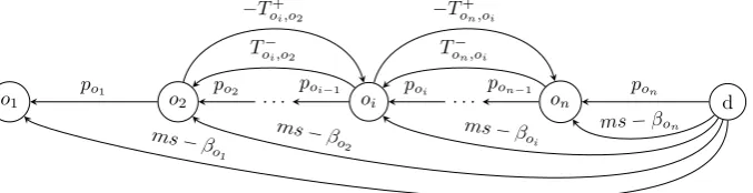
d on . . . oi . . . o2 o1

pon

pon−1 poi

poi−1 po2

po1

To−n,oi

−To+n,oi

To−i,o2 −To+i,o2

ms−βon

ms₋_β

oi

ms₋ βo₂

ms₋_β

[image:20.595.157.496.130.217.2]

o₁

Figure 2.5: Late event time graph

early event time(ET(o)) and thelate event time(LT(o)), denoting the earliest time at which eventocan occur and the latest time at which eventocan occur without delaying the completion of the overall project respectively. The early event times correspond to the earliest possible starting times we determine for operations as discussed above. From these earliest possible starting times we find a makespanms for the schedule, the maximum completion time. The late event times then correspond to the latest possible time each operation can start without increasing the makespan of the schedule. Determining the late event times is done in a similar fashion to determining the earliest possible starting times, through solving a longest path problem.

Given an ordering O~ = (o1, o2, . . . , on) of operations, we can define the late

event time of an operationoi as follows:

LT(oi) = min

          

LT(oi+1)−poi

LT(oj)−To−i,oj ∀oj: (oi, T

−_{, T}+₎ ∈Roj

LT(oh) +To+h,oi ∀oh: (oh, T

−_{, T}+₎_∈_R

oi

βoi

2.1

for i= 1,2, . . . , n−1. Note that the last operation on cannot start any later

thanms−pon and so we setLT(on) =ms−pon. For all other operationsoi, we now have to find the values ¯loi, which represent the minimum amount of time that has to pass between their start andms. Similar to the case for the earliest starting times, we define a corresponding graph to find these minimum amounts of time. We begin by adding a dummy vertexd, corresponding to an operation that starts directly after the schedule has finished atms. Furthermore, we add a vertex for each operation in the ordering. We add an arc betweendandon of

lengthpon and an arc betweenoi+1 andoi of length poi fori= 1,2, . . . , n−1. For each operation o we add an arc between o and every related operation or

of length T_o,o−_r and an arc betweenor and o of length −To,o+r. Finally we add an arc betweendand each operationo of lengthms−βo, to respect the latest

possible starting time βo of operation o. We note that the longest path ¯lo

betweendand vertex oin this graph, corresponds to the minimum amount of time that has to pass between the start ofoandms. We can now defineLT(oi)

byLT(oi) =ms−l¯oi. Figure2.5illustrates an example of such a graph. The early and late event times allow us to define free float andtotal float.

Definition 2.3.1. The Free Float of an operation oi, F F(oi), is defined as

(21)

Definition 2.3.2. The Total Float of an operation oi, T F(oi), is defined as

follows: T F(oi) =LT(oi+1)−ET(oi)−poi.

Until now we have looked at the amount of float available when the makespan has to stay the same. However, makespan minimization is only the secondary objective. Our primary objective is to maximize the number of jobs scheduled. Therefore, if we want to examine by how much the duration of an operation may increase without leading to infeasibility, we are interested in the available float of the operations where the given sequence stays feasible, but the makespan is allowed to increase. For this purpose we introducelatest feasible event time (LF T(o)). This corresponds to the latest possible time an operation can start without making the schedule infeasible. These times can be determined by solving the same longest path problem as we did to find the late event times, only now we note that the last operation can’t finish any later thanβon+pon, instead of ms. If we replace ms by βon +pon in Figure 2.5 we obtain the graph used for finding LF T(o). The longest path ˜lo between d and vertex o

in this graph, corresponds to the minimum amount of time that has to pass between the start of o and βon +pon. This allows us to define LF T(o) by

LF T(o) =βon+pon−l˜o. We can then use this quantity to definefeasible float.

Definition 2.3.3. The Feasible Float of an operationoi,P F(oi), is defined as

follows: P F(oi) =LF T(oi+1)−ET(oi)−p(oi).

When the duration of an operation changes, the operations preceding it should be fixed in place, meaning their starting times, early event times, late event times and latest feasible event times are all the same and can no longer be changed. The reason is that at that point these operations are too close to their execution time to be adjusted (or have already been processed). These fixed operations may influence the time windows of operations that still have to be scheduled though. Therefore, we do have to include them when determining the earliest, latest and latest feasible event times of later operations. Now we can use these three measures to determine the effects of the change in duration.

Let us consider operationoiwhose duration changes frompoi top

0

oi =poi+ ∆oi. We then distinguish the following cases:

Case 1: F F(oi)≥∆oi

If this is the case then poi can increase by ∆oi without affecting the rest of the schedule. By definition,F F(oi) =ET(oi+1)−ET(oi)−poi, soET(oi+1)−

ET(oi)−poi ≥∆oi. Now sincep

0

oi =poi+∆oi, we haveET(oi+1)≥ET(oi)+p

0

oi and so the given schedule remains feasible. In this case we don’t need to take any action.

Case 2: T F(oi)≥∆oi> F F(oi)

If this is the case then an increase ofpoi by ∆oi makes the schedule where every operation starts at its earliest possible starting time infeasible, due to ∆oi >

F F(oi) the same derivation as in case 1 would yield ET(oi+1)< ET(oi) +p0oi. However, sinceT F(oi)≥∆oi and T F(oi) = LT(oi+1)−ET(oi)−poi, we find that the following operation can still start at or before its latest possible starting timeLT(oi+1). From the definition of the latest possible starting times it then follows that the schedule remains feasible and the makespan is not altered.

Case 3: P F(oi)≥∆oi > T F(oi)

(22)

the same ordering and makespan infeasible. Since the following operation will not be able to start at or before its latest possible starting time. However, since P F(oi) ≥ ∆oi there does exist a schedule with the same ordering, but greater makespan that is still feasible. From the definition of feasible float

P F(oi) =LF T(oi+1)−ET(oi)−p(oi), we find that the following operation can

still start at or before its latest feasible starting time, it then follows from the definition of latest feasible starting time that a feasible schedule exists on this ordering.

Case 4: P F(oi)<∆oi

If this is the case thenpoi can’t increase by ∆oi without causing the schedule to become infeasible, because the following operation will not be able to start at or before its latest feasible starting time. In this case we can’t simply move operations back. We have to perform rescheduling and perhaps reject this or upcoming jobs.

Based on the above discussion, we define the robustness of a schedule in terms of feasible float. We define the feasible float of a schedule S = (A, s) as the smallest change in duration of any operation belonging to a job inJAthat makes the schedule infeasible.

Definition 2.3.4. The feasible float of a schedule S, P F(S), is defined as follows: P F(S) = min{P F(o)}over allobelonging to a job inJA_{. Furthermore,}

we call solutionS1 more robust than solutionS2 ifP F(S1)> P F(S2).

Complexity

In the following we discuss the computational complexity of the considered scheduling problem. Specifically, we proof the following theorem.

Theorem 2.3.1. The stated scheduling problem is NP-Hard in the strong sense.

Proof. We show its NP-Hardness by a reduction from 3-PARTITION. First we introduce the 3-PARTITION problem. Given a multiset of 3m integers

S = {x1, x2, . . . , x3m}, the problem is to decide whetherS can be partitioned

into m disjunct subsets S1, S2, . . . , Sm such that the sum of the elements of

each subset is equal, i.e. P

xi∈Skxi = B for all k ∈ {1, . . . , m} where B = (P

xj∈Sxj)/m. The subsets S1, S2, . . . , Sm must form a partition in the sense that they are disjoint and coverS. Given an instanceS={x1, x2, . . . , x3m} of

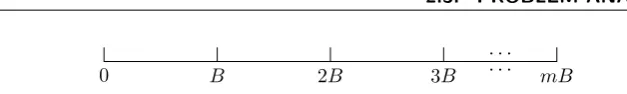
3-PARTITION, we define a corresponding instance of the scheduling problem with 4m jobs. The first m jobs are dummy jobs di each consisting of one

operation odi with the following parameters: podi = 0, αodi = βodi = iB,

i = 1,2, . . . , m. The remaining 3m jobs each consist of one operation oj with

the following parameters: poj = xj, αo = 0 and βo = mB, j = 1,2, . . . ,3m. We note that the dummy jobs partition the timeline in m separate pieces, as depicted in Figure 2.6. A solution to this scheduling problem in which every job is scheduled and which has a makespan of mB will have each of the m

pieces of the timeline completely filled with operations, since the sum of the processing times of the operations ismB and each of the mpieces is of length exactlyB. If we define Si to be the set of operations starting between (i−1)B

andiB, the setsS1, S2, . . . , Sm are disjoint and cover the set of all operations.

Furthermore P

(23)

0 B 2B 3B . . . . . .

[image:23.595.100.414.102.149.2]

mB

Figure 2.6: Timeline partitioned by dummy jobs

any optimal solution in which not every job is scheduled corresponds to a no-instance of the corresponding 3-PARTITION problem. Since we optimize with respect to the amount of jobs scheduled, the only reason for a job not to be scheduled is that it does not fit. This implies there is no distribution of the jobs over the pieces of the timeline such that each of them is exactly filled. Any solution with all jobs scheduled but makespan greater than mB will have an operation that starts at exactly mB, since operations cannot start after mB

(due to βo = mB) and any operation starting before mB will have to finish

beforemB as well (due to the dummy operationdm starting atmB). We can

then use the same argument as in the case where not all jobs are scheduled to show this also corresponds to a no-instance of the corresponding 3-PARTITION problem. Combining these three results shows that we have a yes-instance for 3-PARTITION if and only if we find a solution in which all jobs are scheduled with makespanmB to the corresponding scheduling problem. Since 3-PARTITION is shown to be NP-Hard in the strong sense [5], so is our scheduling problem.

2.3.3 Duration Change Problem

In this subsection we discuss the duration change problem in greater depth. We consider the input to the problem and discuss what makes up a solution.

Input

In a given schedule of the scheduling problem, each operation represents a burst to be processed by the antenna. Shortly before this burst has to be processed parameters for the burst are determined. These parameters can influence the duration of the burst. When this is the case and the burst duration is affected, we have to solve the duration change problem. This may lead to an updated schedule which is being executed from that point on. Shortly before the next burst is scheduled to be transmitted according to this updated schedule, param-eter calculation is again performed and, if necessary, the schedule is updated again. In this manner we iteratively change the schedule by solving a sequence of duration change problems. As a consequence, the input to the duration change problem consists of a schedule S = (A, s) as defined in Section 2.3.2 and an altered processing timep0_o for one operationoin the schedule.

Solution

A solution to the duration change problem consists of a (possibly) modified schedule which accommodates the change in duration. More formally, the so-lution to the problem consists of a new scheduleS0= (A0, s0), whereJA0 ⊆JA

(24)

the same methods as discussed in Section 2.3.2 can be used to compare the quality of two solutions.

Complexity

(25)

Methods

In this chapter we discuss possible solution approaches to the scheduling problem as well as the duration change problem.

3.1 Scheduling Problem

In this section we discuss the possible solution approaches to the scheduling problem. We consider different kinds of approaches and draw a comparison between them.

3.1.1 On-Line

In the previous chapter we stated that requests for jobs arrive over time which makes our problem an on-line problem. Jobs arrive continuously over time, however we do require them to be requested some amount of time before they are allowed to start. Let us call this time the minimum request delay and denote it bymrd. Since we do not want the machine to be idle and since jobs

can start shortly (the minimum request delay) after they are requested, we can’t postpone making scheduling decisions. If there are requested jobs available, we always want to have jobs scheduled for the immediate future. On the other hand we don’t want to commit to a certain schedule too far in the future, due to the possibility of higher priority jobs being requested in the near future. This means that in the extreme case it may happen that we have to determine a new schedule every mrd time units (in the case where each time a new job

arrives directly after determining the schedule), to ensure the machine does not become unnecessarily idle and to ensure we make decisions about arriving jobs in time. Let us call the ith _{time we determine a schedule the} _ith _scheduling run, letti denote the time at which the ith scheduling run takes place and let

ci denote the time between the (i−1)th andith scheduling run: ci=ti−ti−1. At time ti we have to consider the schedule we have so far, which in general

extends beyondti, and at the least the requests for jobs that wish to start before

the next scheduling decision atti+1. Making these scheduling decisions takes a certain amount of time. The exact amount depends on the current schedule, the amount of requests, the amount of operations each requested job consists of and the level of inter-relatedness (in terms of the relations discussed in Section2.2.1) between the operations. Letsi denote the maximum amount of time required

(26)

# αo βo po priority

1 0 0 li/5 1

2 0 li li/5 5

3 0 li li/5 5

4 0 li li/5 5

5 0 li li/5 + 2 5

[image:26.595.225.415.125.224.2]

6 li+ li+ 2 5

Table 3.1: Operation parameters for Example 3.1.1

ti+si ti+li

1 2 3 4 5

6

[image:26.595.158.483.255.322.2]

Low priority High priority

Figure 3.1: Resulting schedule for Example 3.1.1

that wish to start earlier our decision may not be available in time. Furthermore we have to consider each job that wishes to start beforeti+1+si+1, because in the next scheduling run it may be too late to make a decision for these jobs. All jobs we consider that start afterti+1+si+1 may have to be reconsidered in the following scheduling run. Letli denote the amount of time we look ahead, that

is, we consider in the ith _{run jobs whose starting time window overlaps with} [ti+si, ti+li]. As we have seen li has to be chosen in such a way that jobs

that wish to start beforeti+1+si+1are considered. This is represented by the following constraint: li≥ti+1+si+1−ti. It remains to determine appropriate

values for theli. Before we deal with this problem, we first note that for every

finite value of li we can construct an example where a better solution can be

found by increasingli. The following example illustrates this fact:

Example 3.1.1 Consider 6 jobs, each consisting of a single operation. The parameters for these operations are specified in Table3.1. The priority listed is the priority of the corresponding job. In this example we consider ti+si

to be 0. The last job (number 6) won’t be considered in the first scheduling run because its starting time window does not overlap with [0, li]. In the next

scheduling run (somewhere beforeli, but after 0) we do consider job 6, at this

point job 1 is fixed though. This means we have to reject job 6. In the optimal schedule we would have rejected job 1, which has a lower priority than job 6. Figure 3.1 shows the resulting schedule, job 6 is shown hovering above it’s desired location.

For some systems choosingli sufficiently large that all jobs are always

consid-ered may be appropriate, e.g. if all requests are made shortly before they wish to start. We should note that the scenario from the example can still occur; if job 6 is requested after the scheduling run, the outcome is the same. In a system where all requests for a long period are made at the start of the period, setting li in the above mentioned way may cause the processing time required

(27)

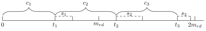
0 t1 s1

mrd t₂

s2

t3 s3

2mrd

[image:27.595.104.438.125.176.2]

c1 c2 c3

Figure 3.2: Scheduling intervals

the schedule to be executed. In a system where requests arrive over time the primary focus should be on obtaining a good schedule for the immediate fu-ture (until the next scheduling run). The operations that make up the schedule over this timespan are the operations that have to start processing shortly and can’t be adjusted anymore. Furthermore, the more distant future is uncertain; that is to say, there may be additional requests which cause us to change the schedule in the future. This has the potential to render decisions we make now, based on our current information, obsolete and even counter-productive. Take for instance our example (Example 3.1.1); if we had considered every job in the first scheduling run, we would have rejected job 1 and accepted job 6. If a request then came in afterwards for a job of priority 10 that had to start at exactly li+ 2, we would have to reject job 6 in favour of this new job and we

could have just scheduled job 1, but now both jobs are rejected. This leads us to conclude that the concrete value for theliparameters should be determined

based on the system the scheduler is used in.

If we have chosen the li values, in each scheduling run, we have to solve

an off-line version of the problem which we discussed in Section 2.2.1. In the off-line version of the problem we have a set of requested jobs and a current schedule to consider. In this context, we should note the relation between ci

and si. If we assume the amount of requests that wish to start in an interval

is proportional to the size of that interval, then the larger we choose ci, the

longer it takes to perform the scheduling and the greatersi will be. However,

ci+si should be smaller than or equal to the minimum request delaymrd, as

the following example shows.

Example 3.1.2 Let ci +si > mrd and consider a job request arriving

im-mediately afterti−1 which wishes to start atti−1+mrd. As the job is only

considered in the next scheduling run starting atti, this means that the

de-cision on whether or not to schedule this job is not made until ti+si which

equalsti−1+ci+si> ti−1+mrd, which may be too late.

This places an upper bound on the value ofci. On the other hand we do not want

to chooseci too small. In the (i−1)th scheduling run we consider each job that

has a starting time window that overlaps with the interval [ti−1+si−1, ti−1+ li−1]. If we choose a small value for ci = ti−ti−1 then that implies we are solving roughly the same problem many times. Whenci is small compared toli

the amount ofnew jobs in each scheduling run is relatively small. The majority of the jobs were already available in the previous scheduling run. Figure 3.2

(28)

3.1.2 General Solution Approach

In the previous chapter we have proven the scheduling problem to be NP-Hard in the strong sense (Theorem2.3.1). In combination with the fact that we have a very limited amount of time to solve our scheduling problem, this leads us to conclude that an exact solution method is infeasible. This conclusion is backed up by the findings in [1]. Therefore, in the following we focus on heuristic solution methods to find a best possible solution in the time available.

As we have seen in the previous subsection, our scheduling problem consists of solving many small instances of the off-line version of the problem. Thus, to solve our scheduling problem we have to solve a series of these off-line schedul-ing problems. In this subsection we discuss the general outline of a solution approach to these off-line scheduling problems.

We can roughly divide the set of possible approaches in two: constructive approaches and local search approaches. Constructive approaches build a solu-tion by starting with nothing and adding jobs one at a time, until no further jobs can be added. Local search approaches work by starting with some initial solution upon which they improve by making small changes to the solution to obtain different (better) solutions. For most problems finding an initial solu-tion for a local search procedure is quite simple, however, for our problem even finding an initial feasible solution is not simple, since we can’t simply take a random ordering of the operations (that will likely be infeasible). Therefore, we need to use a constructive approach to obtain an initial solution, after which we can apply a local search approach to improve on this solution as long as we have time left before the schedule has to start. In this manner we ensure we always have a feasible solution available (assuming there is always enough time to find a solution using a constructive approach). This way we can guarantee the machine does not become idle due to no schedule being available. At the point in time where we have to start executing our schedule, we can use the best schedule found so far. In the next subsections we discuss the various options for constructive and local search approaches.

3.1.3 Constructive Approaches

In this subsection we discuss different methods to find an initial solution using a constructive approach as well as their benefits and drawbacks.

Priority Rule

In Section 3.1.2we explained that in a constructive approach we consider jobs one by one. Our primary objective with regards to solution quality is the amount of jobs scheduled, respecting priorities, as explained in Section 2.2.1. This ob-jective implies that we never wish to reject a higher priority job in favour of any combination of lower priority jobs. The simplest manner to guarantee this behaviour is to consider the jobs in order of descending priority. So when con-sidering a job, the only jobs already scheduled are of equal or higher priority and any job with lower priority has no effect on whether or not the job under consideration is accepted.

(29)

place for them in the ordering. If a given operation does not fit anywhere, we perform backtracking. That is, we attempt to give the preceding operation of this job a different place in the ordering. If no different places for this operation are available, we proceed with the operation before that, continuing until we either find a place for each operation, at which point we accept the job and continue scheduling with the next job, or we can’t find a different place for the first operation, in which case we reject the job and continue scheduling with the next job. This procedure is performed by Algorithm1: Priority Rule which uses Algorithm 2: Operations in window and Algorithm 3: Place before as subroutines. The overall algorithm works as follows: The priority rule starts

Algorithm 1Priority Rule

Procedure_PriorityRule(J, ~O) 1: Sort(J) //Descending by priority 2: for allj∈J do

3: k←0

4: before[·]← ∞ 5: while k <|Oj|do

6: o←Oj(k) //o becomes thekth operation ofj

7: (a, b)←operationsInWindow(o, ~O) 8: i←before[k]

9: i←placeBefore(o, ~O, a, b, i) 10: if i=−1 then

11: if k >0then

12: k←k−1

13: else

14: reject(j)

15: k← |Oj|

16: end if

17: else

18: before[k]←i

19: k←k+ 1

20: end if

21: end while

22: if j was not rejectedthen

23: accept(j) 24: end if

25: end for

by sorting the jobs in descending order of priority (Alg.1l.1) then the jobs are taken one at a time. For each jobj we letkdenotes the index of the operation we are currently considering (Alg.1 l.3). We initialize a value beforefor each operation, this value is used when backtracking to ensure the operation is put in a different place (Alg.1 l.4). Now we take the operations of job j one at a time in the given order and for each operation o we begin by determining the operations in the current ordering whose starting windows overlap with the starting window of o. This is performed by calling the operationsInWindow

procedure (Alg.1l.7).

(30)

Algorithm 2Operations in Window

Procedure_{operationsInWindow}(o, ~O) 1: i←0

2: a, b← −1 3: while i <|O~|do

4: r←O~(i)

5: if there existsxsuch thatx∈[αo, βo] andx∈[αr, βr]then

6: b←i

7: else

8: if b <0 then

9: if βo< αrthen

10: a←i

11: else

12: b←i

13: end if

14: else

15: break

16: end if

17: end if

18: i←i+ 1 19: end while

20: if b < athen 21: b←a

22: end if

23: return (a, b)

Algorithm 3Place Before

Procedure_placeBefore(o, ~O, a, b, i) 1: i←min(i, b)

2: while i≥ado

3: O~ ←(o1, o2, . . . oi, o, oi+1, oi+2, . . . , on)

4: if BellmanFord(graphRepresentation(O~))then

5: return i 6: else

7: O~ ←O~ \ {o} 8: i←i−1 9: end if 10: end while

(31)

of the last operation whose starting window ends before the starting window ofo

begins and the index of the last operation whose starting window overlaps with the starting window ofo. It does this by initializing the indices to−1 (Alg.2l.2) and then iterating over the ordering. For theith operationrfrom the ordering we check ifr’s starting window overlaps with that ofo(Alg.2l.5). If it does, we set the end index,b, tor’s indexi. If it does not, we check ifb <0, because if

b <0 thenbhas not been changed since it has been initialized, meaning we are either still before the first operation whose starting window overlaps with that ofoor none of the operations in the ordering has a window that overlaps with that ofo and this is the first one after the window ofo. If the former is the case, we set the begin index, a, to r’s index i (Alg.2 l.10). If the latter is the case, we set the end index,b, tor’s indexi(Alg.2 l.12). If b≥0 then we have encountered an operation whose starting window does not overlap with that of

oeven though in the past we have found such operations. This means that at this pointaandbare set as the begin and end indices correctly and so we stop iterating over the operations and return the indices we found (Alg.2 l.23). If we have iterated over all of the operations in the order without this occurring, we check if b < a, i.e. if the end index is smaller than the begin index. This only happens if the begin index, a, has been increased while the end index, b, has not. This means all of the operations have starting windows that occur completely before that ofo. In this case we set the end index equal to the start index and return the pair.

We continue in the PriorityRuleprocedure. Now that we have the begin and end index of the “overlapping operations” the place for the operation can be determined. For this purpose the procedureplaceBeforeis used. It is given the current operation, the current ordering, the begin and end indices as computed byoperationsInWindowand the valuebeforediscussed above as an argument. The placeBefore procedure determines a place for the operation in the ordering before the index stored inbefore for this operation. It first tries to insert the operation at the last possible place, i.e. the minimum of the value in

before and the end index computed by operationsInWindow (Alg.3 l.1). It does this by adding the operation in the ordering (Alg.3 l.3), creating a graph representation for this ordering and then use the Bellman-Ford algorithm to determine whether a feasible solution exists (Alg.3 l.4). If a feasible solution exists, the place where the operation was inserted is returned (Alg.3l.5). If no feasible solution exists we attempt to insert the operation in an earlier place. If we can’t find any place to insert the operation, a value of −1 is returned (Alg.3l.11).

Back in thePriorityRuleprocedure, we check if a place was found for the operation (Alg.1l.10). If a place was found, we store the index we found for the operation as the new value for before for this operation and move on to the next operation (Alg.1 l.18-19). If we have not found a place for the operation, we check if this is the first operation for this job (Alg.1 l.11). If it is the first operation, we reject the job and move on to the next job (Alg.1l.14-15). If this is not the first operation, we track back to the previous operation for this job (Alg.1l.12). If all operations have been processed and the job was not rejected, we accept the job and move on to the next job (Alg.1l.22-23).

(32)

procedure has a runtime complexity ofO(n) (wherendenotes the amount of op-erations), the while loop is executedO(n) times and all of the statements inside of the loop can be performed in constant time. TheplaceBeforeprocedure has a runtime complexity ofO(n4), the while loop is executedO(n) times, creating the graph representation requires O(n2) time and the Bellman-Ford algorithm runs in O(n3) time. The other operations only require constant time, making the total running time O(n4_{). The runtime complexity of the}

PriorityRule

procedure isO(n5_{). Sorting requires}_O_(|_J_|_log_|_J_{|) time, everything inside of}_both loops is executedO(n) times. We have just seenoperationsInWindowrequires

O(n) time andplaceBefore requires O(n4_{) time. The rest of the statements} require constant time to be executed. This brings the total toO(n5_).

Shifting Bottleneck Heuristic

One popular heuristic in scheduling is the shifting bottleneck heuristic[6]. Before we describe how this heuristic can be applied to our problem, we first introduce a problem to which the shifting bottleneck heuristic is often applied, the job shop scheduling problem. An instance of the job shop scheduling problem con-sists of a set of machines and a set of jobs each of which has to be processed on a subset of the set of machines in a certain order. A job can only be processed on one machine simultaneously and the machines can only process one job si-multaneously. The aim is to find a schedule which obtains the optimal value with respect to a given objective function. This problem is covered extensively in literature, because it has many practical applications and turns out to be a very hard problem.

The general idea of the shifting bottleneck heuristic is to find a sequence of jobs for the machines one by one. The order in which the machines are considered is determined by finding the bottleneck machine in each iteration. The manner in which this machine is found depends on the objective function. Finding an optimal (locally) sequence for this single machine is a much simpler problem than solving the overall problem. After a sequence has been found for the bottleneck machine, the other machines are re-optimized, i.e. an optimal sequence is determined for them again, one at a time while keeping the sequences of the other machines fixed. These steps are repeated until a sequence for all machines is found.

(33)

The local search is performed by reinserting jobs into the schedule. Let

S = (A, s) denote the schedule after a job j is added. We then iteratively, for each job a ∈ JA\ {j}, remove all the operations o ∈ Oa from the ordering

~

O. Then we reinsert the job using the same mechanism as in the priority rule. We note that this does not lead to any rejections, since the situation before removal always remains feasible. Additionally we try to insert every already rejected job r ∈ J \JA _{into the schedule using the same mechanism as in}

the priority rule. The complexity of this iterative improvement procedure is

O(n5_{), due to the fact that for every operation belonging to a job preceding}_j (in descending order of priority)placeBeforeis invoked. There areO(n) such operations and each invocation of placeBefore requires O(n4_{). The iterative} improvement procedure is executed once for every job, therefore the total added running time, relative to the priority rule, is O(|J| ·n5_{). We have seen in the} previous subsection that the priority rule requiresO(n5), therefore the shifting bottleneck heuristic requiresO(|J| ·n5+n5) =O(|J| ·n5).

Comparison

It depends greatly on the relative performance of the local search approach employed after finding an initial solution which method should be used for finding the initial solution. If the local search approaches are able to quickly find superior solutions the best option would be to just use the priority rule, since this provides a solution faster and leaves more time for local search. If on the other hand the improvement made by the local search approach is small, it is better to spend a little more time finding a better initial solution. How well the local search approaches perform depends on the solution space and the initial solution found. It is therefore very hard to decide which choice is best based purely on theory. Therefore we test different combinations of initial solution methods and local search approaches on a variety of scenarios to obtain a good comparison. These test results are presented in Chapter6.

We should also note that the runtime complexities obtained in this section paint a somewhat distorted picture. In practical situations the size of the in-tervals discussed in Section 3.1.1 are small, this also makes it likely that the amount of operations is small. Thus the smaller order terms and coefficients we are ignoring in the asymptotic analysis can actually have a great impact on the running time.

3.1.4 Local Search Approaches

(34)

Example 3.1.3 We consider a sequencing problem with 3 jobs: j1, j2 and j3 with p1 = 8, p2 = 5 and p3 = 3. We wish to minimize the sum of the completion times. Given an ordering of the jobs, we can easily find the start times for each job by starting the first job at 0 and consecutive jobs as soon as the preceding job finishes. Consider the ordering j1, j2, j3. The sum of completion times for this solution is p1+p1+p2 +p1 +p2 +p3 = 37. Let us consider the local search heuristic where we manipulate solutions by swapping two adjacent jobs. This leads us to a neighbourhood consisting of two solutions, obtained by swapping j1 and j2, and j2 and j3 respectively. The first swap leads to solution j2,j1, j3 with sum of completion timesp2+ p2+p1+p2+p1+p3 = 34. The second swap leads to solution j1, j3, j2 with sum of completion times p1+p1+p3+p1+p3+p2 = 35. For both of these solutions we could then define a neighbourhood again, attempting to find better solutions. If we had instead chosen to manipulate solutions by only swapping non-adjacent jobs, we would have found a different neighbourhood for our initial solution, consisting solely ofj3,j2,j1with a sum of completion times ofp3+p3+p2+p3+p2+p1= 27.

We call the method of manipulating solutions the transfer function. The differ-ence between local search heuristics is in the way the next solution is chosen from the neighbourhood. In the next subsections we discuss different local search ap-proaches, afterwards we discuss possible transfer functions for our scheduling problem.

Descent methods

A descent method starts at a given feasible initial solution and iteratively chooses the first neighbour it encounters with better objective function, un-til the objective no longer can be improved. It can also be modified to choose the best among its neighbours instead of the first it finds or to take the best alternative from some random sample of neighbours. The problem with this heuristic in general is that it stops at the first local optimum, which can be far away from the global optimum and which depends greatly on the initial solu-tion. The main advantage is that in general it converges to this local optimum fairly fast.

Simulated Annealing

(35)

algorithm becomes more and more likely to choose neighbours with a better ob-jective value. Allowing the algorithm to select neighbours with worse obob-jective values helps to avoid getting stuck in a local optimum. Even when the tem-perature gets close to 0 the probability of moving to a neighbour with a worse objective value stays positive (even though it tends to 0). Usually the algorithm is terminated when we are within some reasonable bound of the optimum or we reach some self-imposed bound on computational effort. Since we usually have a very small amount of time available to perform a local search heuristic, we need to choose our parameters very carefully to minimize the probability of ending up with a worse solution.

Genetic Algorithm

A genetic algorithm[8] starts with a random set of feasible solutions called the first or initial population. It then selects a small subset of this initial population (typically those with good objective values). This subset is then transferred to the next population. The rest of this new population is filled with offspring from this subset. The offspring is created using some function that combines two so-lutions into a new one which has attributes of both. Finally some additional solutions are selected from the previous population and added after they have been mutated. Mutation is achieved by randomly changing the solution, still obtaining a feasible solution. This process is repeated until a suitable solution is found or a bound on computational effort is reached. The introduction of mutation ensures the algorithm does not immediately converge to a local mini-mum. This method differs from our description of a local search heuristic in the sense that it works with sets of solutions and that there are multiple transfer functions. Mutation can be seen as a regular transfer function, combination is different since it requires two solutions as input. The main concept of finding new solutions by making small changes to (a set of) other solutions remains the same though. The main difficulty in this approach is maintaining feasibility through combination and mutation.

Transfer Functions

(36)

add previously rejected jobs to the schedule.

Comparison

It depends greatly on the amount of time we have available to run our local search heuristic, which local search heuristic is most suited for our problem. The descent algorithm likely performs better in the initial stages than the simulated annealing or genetic approach. Later on the latter two will catch up though. Tests have to show which heuristic is most suited. A parameter could be used to characterize which heuristic should be used for which specific system. This could be performed automatically, for instance by determining the quality of local optima or depending on the amount of time left. Alternatively the parameter could be determined for a system when it is designed. A search radar is much more predictable and easier to schedule than a complicated multi-function radar for instance. So it is likely that in the search radar there is a greater amount of time available to perform a local search heuristic, thus favouring the simulated annealing or genetic approach. Whereas for the multi-function radar finding an initial solution might take longer, leaving less time for local search, thus favouring the descent approach.

3.2 Duration Change Problem

In this section we discuss approaches to solving the duration change problem as defined in Section2.3.3. In Section2.3.2we defined robustness in terms of float. These concepts also allow us to decide upon an appropriate response to a certain change in duration. For the following we consider the case that operationoihas

a change in duration frompoi top

0

oi =poi+ ∆oi.

The first three cases discussed in Section 2.3.2can be handled by adjusting the starting times of operations. We can maintain the same ordering and only need to determine a new set of starting times. In the fourth case there is no feasible schedule using the current order with the new durations. This leaves us with the following options: a) change the order; b) reject a job or some jobs; or c) leave the schedule infeasible. There is no guarantee that changing the order works, since there may not be an ordering of these operations with these durations which supports a feasible schedule. We may also attempt to reschedule the operations after the affected operation, which may lead to a new schedule without requiring rejections. Depending on how quickly we can eventually perform the scheduling procedure, this may or may not be feasible in the time available. If we need to reject a job, this means that the feasible float of the changed operation oi is not large enough to allow the change. As

the feasible float is defined byP F(oi) =LF T(oi+1)−ET(oi)−p(oi) and since

we can’t influence ET(oi) anymore (at this point the past is already fixed),

we are left with LF T(oi+1), the latest feasible starting time of the operation following oi. This latest feasible starting time is determined by the operations

(37)

operationsCi on the longest path such that their removal increasesLF T(oi+1) enough for the schedule to become feasible, i.e.,P F(oi) has to be increased such

that ∆oi ≤P F(oi). Furthermore, we want to find the collection of operations with this property whose corresponding jobs have the lowest maximum priority. LetJCi denote the set of jobs to which the operations in Ci belong. That is,

JCi={j∈J|Oj∩Ci6=∅}. Then among all the collections of operationsCiwith this property we wish to find the collection for whichmaxj∈J_Ci(¯pj) is lowest. If

there are multiple collections with the same maximum priority, we choose the one with the smallest amount of jobs in the corresponding set of jobs, i.e., the one for which |JCi| is minimal. If the maximum priority of the collection we find is larger than that of the job thatoi belongs to, we reject the job thatoi

belongs to. Otherwise we reject the set of jobsJCi that the operations we have found belong to.

The last mentioned option is to leave the schedule infeasible. This can be done if the amount ∆o−P F(o) is small and we expect future operations may

have sufficiently lower durations than expected to compensate for this. Whether or not we want to use this option depends on how much risk we are willing to take and on the priority of the job the operation belongs to. If the priority of the job this operation belongs to is low, we risk having to reject a higher priority job later on if the duration of future operations does not decrease sufficiently. On the other hand, if the priority of the job is high the risk of rejecting a higher priority job later on is smaller (since the probability of a higher priority job occurring is lower). To make a decision we need additional information on the probability distribution of the duration of an operation and the amount of risk we are willing to take. These are things that are not necessarily the same for different radar systems though. Therefore, we can’t give a general answer here and merely mention the possibility to implement it in specific systems.

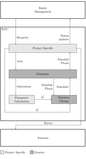
3.3 Architecture

(38)

WFC

Project Specific

Scheduler

Parameter Calculation

Duration Change

Jobs Schedule

Floats

Operations

p0o

Schedule0 Schedule

Floats

p0_o

Requests Status

updates Radar

Management

Antenna Bursts

[image:38.595.176.464.151.680.2]

Project Specific Generic

(39)

them along to the scheduler. The following example illustrates why this setup may be useful.

Example 3.3.1We consider a radar system that has a certain job for which it asks that all operations have to be processed consecutively i.e. each operation has to start when the previous one finishes. The project specific part can modify the operations to enforce this constraint by creating relations between consecutive operations. That is, by creating a relation between operationo2 that directly follows operationo1, that states the minimum time between their starting times is equal to the maximum time between their starting times is equal to the duration of operationo1.

Once these (possibly modified) requests arrive at the scheduler, the actual scheduling occurs. The result is a schedule and a set of floats for each operation. The schedule and float information is sent to the duration change handler, so that it can deal with possible changes in duration. The schedule and float infor-mation is also sent to the project specific part of the scheduler. This allows the project specific part to influence the schedule after it has been created by ad-justing the duration of operations. The following example illustrates a scenario where this is used.

Example 3.3.2Consider a radar system that performs a task which includes one operation that the system would like to perform for as long as possible. This operation still has a limited start window though and there are requests for jobs to start after it with higher priority. Now the requesting party has to choose a certain duration for the operation for it to be scheduled properly. If this is chosen too large, the operation does not fit and the job is rejected. Therefore the duration can’t be chosen as large as the system might like it to be. Now let us assume the scheduler has created a schedule and the job the operation belongs to has been accepted. This schedule, including the float information is sent to the project specific part of the scheduler. The project specific part can now use the floats to determine how much the operation in question can be enlarged without making the schedule infeasible. It can then signal the duration change handler that the duration of the operation has changed by the determined value, which leads to a modified schedule in which the duration of the operation is as large as possible.

(40)

(41)

Approach

In the previous chapter we discussed different methods that could be applied to our scheduling and duration change problem. In this chapter we discuss which methods are actually applicable to our specific problem. Furthermore we discuss the approach we take with regard to testing the performance of the methods we have chosen, both in quality and runtime.

4.1 Method Selection

We discussed different possible methods for both the scheduling and duration change problem in the previous chapter. In this section we determine which of those methods are suitable for our specific problems. We start with the methods for the constructive approach to the scheduling problem.

We only have to consider two options for the constructive approach, the priority rule and the shifting bottleneck heuristic. Both of these methods seem to be applicable to our problem. Computational experiments have to show whether or not one is to be preferred to the other.

There are more local search methods to choose from. We have the de-scent methods, simulated annealing and genetic algorithms. In our scheduling problem the time we have to perform the local search method is very limited. Furthermore, consistently finding the same solution given the same input is important (for testing purposes). Therefore simulated annealing and genetic algorithms aren’t a good choice for our problem, since there is no guarantee that these will always find the same solution if presented with the same input. This leaves the descent methods. Summarizing, we are left with two options for the local search and they are the two different variants of the descent method: choose the first alternative we find which has better objective value(first fit), or consider all possible alternatives and take the best(best fit). Whether the latter alternative is feasible within the time available has to be determined through computational experiments.

(42)

infeasible might be a viable option, while in other systems this might not work. Therefore we only mention the different alternatives, without making a choice.

4.2 Performance Testing

To test the performance of the different methods, we have to implement them and design a framework to simulate requests and parameter calculations. The concrete implementation of these methods and the surrounding framework is discussed in the next chapter. For the testing of the performance of the methods, we then use two realistic scenarios. We use a search scenario and a tracking scenario, because these scenarios allows us to focus on specific parts of the scheduling problem. We run the scenarios 100 times and average the resulting running times to minimize the possible influence of other tasks active on the system.

Search Scenario The first scenario is a search scenario. In this scenario the ordering of the operations is pre-determined. The jobs have to be processed in the given order, and of course the operations that constitute a job always have to be processed in their given order. This means we only have to determine the exact start times for the operations. However, the durations of the operations are subject to change in this scenario. The requests in this scenario are engi-neered in such a way that everything should fit without problems. Therefore, this scenario tests the ability of the scheduling algorithm to handle changes in duration and it allows us to easily check whether or not the solution the scheduling procedure produces is correct, since we know the solution we want to achieve in advance.

Tracking Scenario The second scenario is a tracking scenario. We assume the scenario is executed on a phased-array system. In this scenario there are 5 different parties making requests. They are unaware of each other and can therefore each claim up to 100% of the radar timeline. This means a lot of jobs have to be rejected. There are no constraints on the ordering of jobs though and the duration of operations is known in advance. Therefore, this scenario tests the scheduler’s ability to decide which jobs to accept and which jobs to reject. It should also prove to be computationally more complex, since the order is not known in advance. The fact that the order is not known in advance does make it more difficult to determine the quality of the solution the scheduling algorithm finds. Ideally we would like to compare the solution to the global optimal solution. This is very hard to compute though and we don’t have a direct way of doing so at the moment. Therefore we use the degree to which the radar timeline is filled as a measure of quality.

(43)

Implementation

In order for us to be able to draw conclusions regarding the methods outlined in Chapter3, we need to perform computational experiments to determine the feasibility and performance of these methods. In order to carry out these ex-periments, we require an implementation of the methods as well as a framework to simulate requests being made and parameter calculation. In the following sections we discuss this implementation in greater detail. Java is used for the implementation, mainly based on the familiarity with that language.

5.1 Algorithms and Optimizations

In this section we discuss the different algorithms and some optimizations that were applied. We first discuss the constructive approaches and afterwards the local search algorithm.

5.1.1 Constructive Approaches

We consider only two constructive approaches, the priority rule and the shifting bottleneck heuristic. We begin by discussing the priority rule, since only a small modification is required to turn the priority rule into the shifting bottleneck heuristic.

Priority Rule