Computational analysis of multi storey framed deck structures

University of Warwick institutional repository:

http://go.warwick.ac.uk/wrap

A Thesis Submitted for the Degree of PhD at the University of Warwick

http://go.warwick.ac.uk/wrap/74136

This thesis is made available online and is protected by original copyright.

Please scroll down to view the document itself.

COMPUTATIONAL ANALYSIS OF MULTI-STOREY FRAMED DECK S'rRUCTURES

by

Derek C. Breeden

A Thesis

submitted to the University of Warwick for the Degree of Doctor of Philosophy.

The author wishes to thank Mr. J. Wright for his advice and supervision of the work and Mr. D. Anderson and Mr. M. Larcombe for their help and encouragement. He also wishes to express his thanks to l~ss P. Sotheran who prepared the typed manuscript

ABSTRACT.

A new approaoh to the analysis of three-dimensional framed structures whose prismatio members are interconneoted by slab floors is presented. The method is illustrated by the oomputer program described. The structures are restricted to those of an orthogonal nature with rigid, 1nterc~ected elements. The method of solution is a stiffness matrix approach utilising a

finite element formulation for the in-plane and out-of-plane action of the floor deck. A process of oondensation is applied to the stiffness matrices to reorganise and reduce storage demands. A 'part-structure' condensation is employed floor by floor,

making the process highly suitable for multi-storey structures. Several examples are given to illustrate the use of the program and to demonstrate its versatility. Also the wide range of results obtainable and the methods of presentation are given.

The program is used together with one for a plane frame analysis and one for a rigid, orthogonal, skeletal space frame analysis, both of which are desoribed in this volume, in order to investigate and oompare the solutions obtained for the test frames described. Some results are presented for the investigation

into the stiffening effect of the floor slabs on the bare frame. Also the use of three-dimensional sub-frames for the analysis of beams in a space frame is presented.

LIST OF CONTENTS.

Abstact i

Nomenclature. vi

1 • Introduction.

1.1 Historical and Critioal Review of the Field 1 of Reeearch.

1.2 The Scope of the Proposed Work. S

1.3

The Application of Programs for Elastic ₉ Analysis to Design.

1.4

The Present state of the Proposed Resaerch. 10

1.5

lteferences. 11

2. The Determination of Pointe of Contraflexure Along Tee-beams. 2.1 Introduction.

2.2 Tee-beam Stiffness Matrix. 2.3 Points of Contraflexure. 2.4 Program Implementation.

13

15

18

21 2.5 Example Frame Illustrating the Use of the Tee- 30

beam Program.

2.6 Some Further Test Results Using Tee-beam Program.

2.7 Comments on the Example of Fig. 2.7 and Test Resulte.

2.8 Summary and Conclusions. 2.9 References.

39

3.

Orthogonal Space Frame Analysis.

3.1

Introduction.

3.2

Analysis.

3.3

Program.

3.4

Example Illustrating the Use of Rigid Orthogonal Sp&ce Frame Program.

3.5

References.

4.

Uee of Finite Elements for Slab Stiffness Representation.

4.1

Introduction.

5.

4.2

Plate Flexure.

4.3

Plate Shear - Plane Stress.

4.4

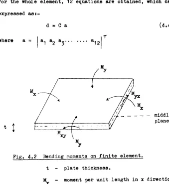
Examples and Results Illustrating the

Use of Finite Elements.

4.5

References.

Rigid Orthogonal Space Frame with Floor Decks.

5.1

Introduction.

5.2

Method of Solution.

5.3

Computational Problema.

5.4

Floor Assembly.

5.5

Supporting-beam Assembly.

5.6

Structure Assembly.

5.1

Solution for Structure Deform&. tions.

5.8

Solution for Member and Element Forces.

5.9

Systems Usage.

5.10

Program Implementation.

43

46

49

54

59

60

61

66

69

16

18

19

81

85

81

92

97

100

101

5.11 Program and Flowoharts. 105

5.12 Note on Sign Convention. 105

5.1~ Test Frames Illustrating the Use and 107 Versatility of the DECK1 Program.

5.14 Verification and Limitation of DECK1 Program. 121

5.15 References. 12~

6. Comparative Elastio Analysis of Test Frames. 6.1 Introduction.

6.2 Test 1.

6.3 Results for Test 1. 6.4 Comments on Test 1.

6.5 Test 2 - Effect of Mesh Conoentration.

124 125 127 132 134 6.6 Comments on Test 2 - Effeot of Mesh Conoentration. 1~9

6.7 Test 3 - Sub-framing. 144

6.8 Test

3 -

Results on Sub-framing. 145

6.9 Comments on Sub-framing Results. 152

6.10 References. 15~

7. Discussion of Decked Frame Solution and Comparative Testing. 7.1 Discussion of the Program and the Method

of Solution Described in Seotion 5.

154

7.2 Advantages and Limitations of the DECl(1 Program. 156 7.~ Discussion of Comparative Test Results 157

of Section 6.

8. Summary.

8.1 Summary of Completed Research. 8.2 Suggestions for Future Work.

Appendix - Algol listing of DECK1 program.

Nomenclature.

A - cross-sectional area, transformation matrix.

AX1 (2), AXL1(2) - axial force at end 1(2).

D - elasticity matrix; flexural rigidity.

DEFX(Y,Z) - defleotion in direotion of X(Y,Z) axis.

E - Young's Modulus.

E - strain veotor.

F_X1(2),FX1(2) eto - foroe in X direotion at end 1(2), similarly for Y,Z direotions.

F , F

_x

- in-plane forces on plate element. y

G - shear modulus.

I ,I ,IY,IZ

-

moment of inertia about Y(Z) axis. y

z

J - polar moment of inertia.

K - stiffness matrix.

L - length of side of slab.

M_x1(2),MX1(2) etc - moment about X axis at end 1(2), similarly for Y,Z direotions.

M ,M ,M

x y z Jf , M '

x

Y

II ~ MOM1 (2)

N

p

px(y,z) ROTN ROTX(Y,Z) SHR1(2)

- moment about X, Y, Z axes.

- moment per unit length in X, Y direotion. - twisting moment per unit length.

- moment at end 1(2). - number of nodes.

- load vector, foroe veotor. - load in X(Y,Z) direction. - rotation.

SY1 ,SZ1 ,SY2, SZ2 S , S

_x

_y

s

_xy

U

X,Y,Z X',Y',Z' XC,YC,ZC

X-DIR, Y-DIR

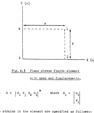
d

dx, dy, dz

n q

t

u

v w

ex(y,z)

- force in Y(Z) direction at end 1(2). - direct stresse8.

- shear stress.

- uniformly distributed vertical load. - member axes.

- structure axes. - X,Y,Z coordinatea.

- displacement in X, Y direotion. - displacement vector.

- di8plaoement in X,Y,Z direction. - number of member8.

- load per unit area. - thickness of 8lab.

- deflection of plate in X direction. - deflection of plate in Y direction.

- shape function; vertical defleotion of plate. - rotation about X(Y,Z) axes.

1. INTRODUCTION.

1.1 Historical and Critical Review of the Field of Research.

The elastic analysis of structures has become a highly complex and extensive region for research. It can range from element or material behaviour to a more macroscopic scale such as total structural behaviour of large multi-storey frames.

Before the advent of computers, analyses for large systems were tedious, being es~ablished using tabular methods suited to the drawing office and they could not be expected to handle complex structures. However, with the arrival of the computer, techniques utilising its attributes were extensively developed. Whereas an increase in the number of equations to be solved made hand solution undesirable, no loss of efficiency is apparent in a computer solution.

The mathematical statement of the structural analysis problem was expressed as a series of simultaneous e~uations in matrix notation, since this was a highly attractive form for the programming of machines. Classical theory was used to obtain equations relating the unknown joint displacements of the structure to the applied loads, the structural properties

1

to be far superior, when applied to more complex structures,

compared with other methodR ~vailable such as moment distribution. Although computer programs were initially developed as

a research tool the eventual aim was for a working design aid and therefore the programming of the technique for practising engine ere became the main objective. Here, the efficiency of programs in continual use became important, and the programming approach became more refined with the influenoe of user

requirements.

Initially a plan~·frame analysis was a straightforward programming exercise once the mathematical formulation had been derived, since generally the computer could handle the demands the analysis made on it especially when symmetry and bandwidth were utilised in the structure matrix. An early program was developed by Livesley1 who, it appears, instigated the development in this direction on a wide scale and his book on I Ma trix MethoJs of structural lUlAlysis' is a sound expose on the subject.

Gelleral purpose programs were soon available but at this stage were confined to plane frame analysis, which proved to be and still proves to be a very useful ru,d readily

implemented aid to the structural designer. Although only an idealisation of three-dimensional behaviour, for design purposes it has proved adequate. However, where a structure does not readily lend itself to simulation by a series of plane frames or the loadinb is not in the same plane as the frame, then the demand is for the next stage, namely space frame analysis and the first extension to a three-dimensional analysis was that fer a skeletal space frame.

With the extension to three-dimensional apace frames the demands on the computer store increased. In the plane frame case only three degrees of freedom at a node are required. Therefore for a frame of N nodes there are 3N equations to be solved. The corresponding etructure matrix for this is 3N x 3N in size, but this is both symmetric and banded, which allows for a much more compact form of data storage. Por a space frame, the number of unknowns increases to 6N and the storage requirements increase alarmingly. This was only a problem

whilst the size of computers was small but with the development of better machines and suitable backing store the problem

became surmountable, enabling three-dimensional skeletal analysis to be undertaken.

However, for more encompassing structural behaviour, research workers now aimed for what might be called 'the

the behaviour of a beam or column member could be defined by the slope-deflection equations. In order to include elements such as floors or walls into the analysis the elastic behaviour or stiffness of these elements would have to be defined. The development of sophisticated techniques such as finite

difference, finite element2, localised Ritz 3 and other variational methods allied to computers has enabled these extra elements

to be incorporated. However, it can be here that the problems start.

The finite difference formulation for the analysis of thin plates can be extended to provide a force/displacement relationship as developed by Croll

4

or Salonen

5

which could be incorporated into a structure analysis, but results provided by this are inferior to those of the finite element method2• This technique enables the complete definition of all the required variables except one, that is the in-plane rotational stiffness of the plate element. Despite this, it does provide the best force/displacement relationships for ease of use in programming for a complete structure analysis.

Thus with the theoretical obstacles removed all would appear straightforward but, as stated earlier, it can be here that the real problems start to occur. In order to formulate the arithmetic into a systematic solution process for a computer program it is evident that the demands on computer storage can be excessive. Thus it is inevitable that

justifiable, this may be achieved by approximation.

Therefore a new direction evolved where approximate or pseudo-three-dimensional structural behaviour could be handled more easily than the full elastic analysis of a diaphragmed space frame. These approximating tecluliques are usually applied to structures whose nature is such that it diminishes any

error in the approximation.

6

An early approach put forward by Clough was one where the floors were asswned to act as rigid diaphrQb~ and that torsion of the structure could be negleoted. Here, horizontal deflection of frames and wall elemente would be equal, which could result in substantial error. A similar procedure was used by Weaver and Nelson

7

in their paper on 'Three-dimensional analysis of tier buildings' where all joint displacements and all element stiffnesses are considered. However, again the floor slabs were assumed to be diaphragms, rigid in their own plane.

In a paper by Majid and Williamson8 'a method for the analysiS of general complete structures conSisting of a combination of one or more of three basic components of the structure, namely: prismatic members, plate elements subject to forces within the plane of the elements and plate elements subject to out-of-plane forces' is described together with the associated computer program. The process uses a matrix

matricel!, where fi.nite element techniques are used to develop the plate element stiffness,

The program described is very comprehensive, including the analysis of general frames in three-dimensions. However, it does require that all the degrees of freedom are represented in the structure stiffness matrix at the sarne time and because of this storage requirements can soon lead to problema with quite small structures, especially if diaphragm sections are split into many elements. The mathematical analysis is justified by experimental results given in the paper, and it is I!tated that the addition of a floor slab increaeel! by about 25% the in-plane sway stiffness of the bare frame.

The paper by Bond

9

describes a similar analysis and goes on to give information of a program for studying the design of reinforced concrete I!tructures supported on columna. In order to reduce the complexity of the problem, the number of degrees of freedom haa been reduced from the

6

per node in a space frame structure. Here only the flexural behaviour of the slab element has been considered and torsional resistance of the columns has been omitted. An approximation is used to overcome the lack of continuity between beam and slab elements, where beam elements are restricted to only three degrees of freedom.

of analysing two-dimensional panels arranged orthogonally

or obliquely, whose compatibility of displacements is provided

for at panel intersections. tiere a two-dimensional approximation

to the three-dimensional situation is undertaken with the

assumption that certain degrees of freedom in these casee are

not significant. Heavy restrictions are put on the floor behaviour,

where elements are treated as rigid diaphragms of infinite

in-plane and zero transverse stiffness. However, the method does

point to the use of repetitive elements or sections of structure

throughout the space frame.

A different approach to the problem is put forward by

11

Zienkiewicz, Parekh and Teply in their paper on 'buildings

composed of floor and wall panels', where the primary load

bearing action is taken by in-plane forces. The paper demomatratee

this approach by examples and expresses the economy in the adoption

of this form of action. However, it only corresponds to those

structures of the panel nature described, e.g. load bearing

shear wall structures etc •. Thus it is not applicable to

column/beam/slab structures where the bending action is more

predominant.

An approximation of structural behaviour, illustrated

in a paper by

N~jid

and croxton12, enables the 'wind analysis of complete building structures by influence coefficients'.

Conclusions are made that there is a real need for special

purpose programs for the various kinds of three-dimensional

analysis, and also that 'the assumption that the slabs are

rie;id diaphragms can t5Tossly misrepresent their actual

Yet with all these possible approaclles it still appears that one question remains unanswered, that being the comparative merits of these various solution processes. When searohing for a program the designer must choose one to suit his requirements, but will he know what the various progTams will provide and what is more important, will the one he chooses be the most efficient? Thus it appears that any information on the comparative merits of program systems for elastic analysis would be beneficial.

1.2 The Scope of Proposed Work.

With the foregoing background of research in the field of three-dimensional structures it was decided to develop a computer program to analyse a special, though by no means rare, kina

of structure. It was hoped that techniques utilised in the work on Tee-beam analysiS13 would prove fruitful in reducing the problem to a manageable size.

The specification of the kind of structure to be considered was not expected to be restrictive since the nature of the

specialised structure was to be orthogonal, a type which occurs frequently in today's framed buildings. The structure could consist of column and beam elements interconnected by floor elabe. The construction material must be borne in mind since it may aleo influence the nature of the program.

erroneous results12• 1hus it was essential to establish suitable mathematical representation of the floor elements and an jnvestigation into this problem was scheduled, bearing in mind the need for the ease with which element formulation would allow versatility in the floor layout.

The main objective resolved itself into a full

three-dimensional elastic analysis of orthogonal beam/column systems interconnected by elastic plate elements representing the floor deck. The developed program would utilise available mathematical and computa.tional techniques in performing the analysis of multi-storey structures.

It was also decided to investigate the comparative merits of certain approaches to elastic structure analysis using

programs which were available, these being a plane frame analysis, a skeletal space frame analysis and a 'complete structure'

analysis. The results from this work may influence the choice of program type for a particular use, and would enable

conclusions to be drawn as to how three-dimensional behaviour can be r~presented more accurately in a simpler analysis.

1.3

The Application of Programs for Elastic ~1alysis to Design.

It could also be used to investigate the optimisation of a structural layout.

Analysis can be used for the overall structural behaviour in conceptual design or in determining element forces to

facilitate element design. Therefore it is necessary to specify the obJ3ctive in order to set the requirements of the computer program. The mass of results provided by large general purpose programs is not always applicable to certain stages of design and a plane frame analysis would provide the required information in a sufficiently accurate form.

The question of efficiency and economics must be considered when computer programs are to be used as a design tool. Unless the program can be demonstrated to be, in effect, more efficient and/or more economic than the methods i t is replacing, its use cannot be said to be beneficial. The need for its operation to dove-tail into the production side of design work is of particular importance when it comes to user orientated programming. Yet this cannot be an overriding factor such that the programs must be adapted to cater for general office practice. ;lowever, incorporation of a program system should not cause undue interference with the efficient running of the design process.

1.4 The Present state of the Proposed Research.

implemented but only in & prototype form; however, successful use of the program has still been achieved.

Two other programs have been written or adapted, one analysing elastic plane frames and the other skeletal space frames, which were used together with the prototype program in the investigation of different elastic frame solutions.

The comparative frame testing was carried out with the three programs as stated above but the author would have wished to have extended the work in this field. Yet result~ for the tests completed have already shown interesting trends and have proved to be quite enlightening. The approach of considering a limited sub-frame concept in three-dimensions has not been successful but has lead to some encouraging results.

Despite a certain amount of progress being made, it is thought that there is still room for improvement and

refinement to the main program and that further frame testing would eventually lead to beneficial results.

1.5

References.

1. R. K. Livesley - 'Matrix Methods of structural Analysis' Pergamon Press, London

(1964).

2. O. C. Zienkiewicz - 'The Finite Element Method in Engineering Science' McGraw Hill, London

1971.

4. J. G. A. Croll - 'Hermitian Methods for the Approximate Solution of Partial Differential Equations' J. Inst. Math. Applics. (1970) 6, 365-374.

5. F. M., Salonen - 'Rectangular plate bending element the use of which is equivalent to the use of the finite difference method'. Int. J. of Numerical Methods in Engineering. Vol. 1, 261-274 (1969).

6.

R. W. Clough et al - 'structural analysis of multi-storey

buildings.' Proceedings of A.S.C.E. 1964,

90,

ST3,19-34. 7. J. R. W. Weaver

&

M •. F. Nelson - 'Three-dimensional analysis

of tier bnildiIll:,'S'. Journal Str. Div. A.S.C.E. ST6, 1966 (Dec) 385-404.

8. K. I. Majid

&

M. Williamson - 'Linear Analysis of Complete Structures by Computers'. Proceedings of I.C.E. Vol. 38 Oct. 1967, 247-266.

9. D. Bond - 'A Computer program for studying the design of reinforced concrete structures supported on columns'. Proceedinb~ of I.C.E. Vol. 43, June 1969, 195-214.

10. M. C. Stamato

& B.

Stafford Smith - 'An approximate method for three-dimensional analysis of tall buildings'.

Proceedings of I.C.~. Vol. 43, July 1969, 361-379. 11. O. C. Zienkiewicz, C. J. Parekh

&

B. Teply -

trrhree-dimensional analysis of buildings composed of floor and

wall panels'. Proceedings of I.C.E. Vol 49, July 1971, 319-332. 12. K. 1. Majid

&

P. C. L. Croxton - 'Wind analysis of complete

2. 'rilE Di'rllil,INA'rIUN OF POINTS OF CONTIlAF'LEIi.Urlli ALONG

TEE-BEAMS.

2.1 Introduction.

In current computer programs for the elastic analysis of plane frames by the stiffness method, the stiffness of each member of the frame is constant, and where it is desired to include a member of non-uniform cross-section it is necessary to introduce new joints at the pOSitions of the change in

properties.

In analysing concrete plane frames, in a monolithic structure, the beams can be assumed to act as Tee-beams. Here, there is an increase in the beam's stiffness produced by the increase in cross-sectional area of the member. However, since Tee-beam action occurs only in the compression part of the member, the analyst has to choose whether to make the whole, or part of, the beam a Tee-section.

Ii1 the first case no new joints are needed but it may

be that a Tee-beam has been assumed where a hogging moment exists, 1.e. a compression flange has been asswned where the beam is

The changeover pOints are known as the points of contraflexure and are not fixed but, in a fully rigid rectangular structure, depend on the system of loading and restraint on the beam.

In practice it appears that these points are assumed to be at fixed positions on the beam, varying between 0.1 and 0.15 of the length of the beam from its end. It seems that these values have been set by experience and are accepted in codes of practice. However, as there has been little work done in the determination of accurate positions for these points, considering Tee-beam action, a oomputer program was written which ar~lyses plane frames using Tee-bearne and which calculates

the locations of the points of contraflexure. These calculated locations are then used to re-construct the stiffness matrix for the Tee-beam, followed by a re-cycling of the analysi/'!! for

iteration towards accurate location for the points of contraflexure, 'rhe program provides an understanding of how a sophisticated elastic analysis program is implemented. It enables an

investigation into the use of a condensation technique, demonstrating its advantages but also illustrating its drawbacks. The Tee-beam analysis allows the study of the behaviour of a segmented beam, with particular reference to its effect on the bending moment distribution, to be undertaken.

2.2 Tee-beam stiffness matrix.

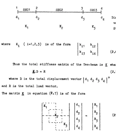
The stiffness matrix of a Tee-beam comprises three element stiffnesses, where the beam is assumed to be composed of three elements or segments. The two end segments are assumed to be acting under a hogging moment and therefore are taken to be rectangular in cross-section, whereas the middle segment is in compression and thus is assumed to have a Tee section. A stiffness matrix is constructed for each segment and the total stiffness matrix of the'beam is obtained by combining the segment matrices.

A compatible matrix for a Tee-beam, of the same fOl~ as that for an ordinary member, is obtained by the removal of the unwanted displacements. This is accomplished by suitable adjustments to the total stiffness matrix to prepare it for a Gaussian elimination procedure

5•

This procedure is stopped as soon as the unwanted displacements have been removed. The

'condensed stiffness matrix' for the Tee-beam is now contained in the total stiffness matrix after this elimination. This

matrix will be the same size as the usual member stiffness matrix. The whole process is illustrated algebraically belowl

Let r

1 be the vector of unwanted displacements, i.e. internal member displacements.

Let r

2 be the vector of retained displacements, i.e. member-end displacements.

K is the stiffness matrix so that

r₁ R1

K.

₌

r_{2 R2}

where K

₌

_{k1 k2}

kT 2

k3

therefore

which is of the usual form K.r

_-

=

_-

R

( T -1 )

where the condensed matrix!

=

k, - k_{2.k1 .k2} T -1 and the condensed load vector

R

=

~

-

k_{2.k1 .R,}

(2.1)

(2.2)

(2.4) (2.5)

It should be noticed that this condensed matrix is load dependent which separates i t from the usual load independent member stiffness matrices, since, when condensing a member matrix, it is necessary to condense the load vector associated with it.

How the condensation process is applied to the total stiffness matrix is not completely self-evident. The actual process is carried out by applying a Gaussian triangularisation routine to the total stiffness matrix of the Tee-beam after it has been re-arranged so that the unwanted and retained displacements are in the vectors r₁ and r

Fig. 2.1 Segmented Tee-beam.

1

I

SEG1 2

I

SEG2 3

I

SEG3

I

4 ~

d

3 d4 Displ

vect

K3 _StH

rna

where Ki

(i=1,2,3)

is of the form

(2.6)

1hus the total stiffness matrix of the Tee-beam is

K

where

I.D

=R

where D is the total displacement vector Id₁ d

2 d3 d4

IT

and R is the total load vector.

The lliatrix! in equation (2.1) is of the form

---1 _d

1 R1

K1

I

-

- I- - T

1 I I d₂ R2

- 1 - ~ ~_

=

I I I _d

3 R3

I 1 I .- - - 1 - - - K

I 3 d

4

R4

I

I . _ _ _ _

(2.1)

(2.8)

Now the actual end displacements of the Tee-beam are containel in vectors d₁ and d

4, leaving d2 and d₃ as the unwanted displacemen" represented by r₁ in equation (2. 1).

It is possible to expand equation (2.A) using the individual segment matrices K. as expressed in equation (2.6) for the total stj

~

[image:27.508.75.459.71.515.2]

k14 + k21

~2

: k13 0 d

2

J

~I

,

_I

k23 k24 + k31: 0 k32 d₃ R3

- -- - -- -

-

- r - - .-- =

(2.9)

k12 0 : k11 0 d₁

R,

0 _k33 I 0

k34 d₄ R4

This is now in the equivalent form of k1 k2

since

Therefore it is now possible to eliminate the unwanted displacements using the Gaussian process.

A

flowohart for the procedure is given in Fig. 2,2, where it is sufficient to note that if the process is operated to a required depth of the stiffness matrix (in equation (2.9») a condensed matrix and load vector will be obtained.

2.3

Points of contraflexure.

L

-

-

--M1

,~)tart

I

i -=

o.

1/JPIV./

'---illS j

>

N + ?

•

I

IA ,

-l<J AI .. >{.J

yes

Stop

Fic;. 2.2 Flowchart diabTam for matrix condensation process.

I f tfle total stiffness matrix is K with load vector R then the

matrix A is as folLows:- A ==

i. e. the las t column of A holds the load vector.

The size of A is ~ N+1.

Fig. 2.3 illustrates the usual form of the bending moment which exists along a typical Tee-beam. It is required of the program to determine the points of contraflexure on those beams being used as Tee-beams. Since these positions are the locations of zero moment along the bearn, the full bending moment distribution along the beam is required. In Fig.

2.3

the points of

contraflexure are indicated by P1 and P2.

The joint displacements and forces are obtained from the stiffness matrix analysis of the plane frame. Therefore the

restraining mO'lellts, J.abelled M1 and M2 in Fig. 2.3, are obtained from this nodal allalysis, and the total moment distribution is the sum of the restraining moment and free bending moment

distributions. ~IUS the only requirement is the so called 'simply supported' moment distribution. This is not readily obtainable from the analysis and extra procedures are necessary to store member loads in readiness for its calculation. Using these loads and member properties the simply supported moment distribution for any member is obtained via the well known formulae for point, uniformly distributed and moment loads, which are built into the program.

Having obtained the total distribution it is necessary to locate the points of contraflexure. Specific values for the moment are stored at N+1 points at intervals of liN along the beam. A search is then made to locate a change of sign between

M and M 1 (the moment values at the ith and i+1th locations).

i i+

.--I

~i

1'\

j~

I liN

1 • •

-xi x. ₁₊ 2

Fi_Q• 2.4 Linear interpolation, after interval search

1

x.

1

of bending moment for change in sign. Exact moment ,curve.

Linear approximation to moment curve. Beam length.

ith x coordinate along beam.

by a sim:,le linear interpolation between the interval, as illustrated in Fig. 2.4. The position obtained is an

approximation but has proved sufficiently accurate for general analysis purposes. Due to the usual shape of the bending moment curve, the slope between an interval is fairly shallow, tending to a straight line, and therefore a linear interpolation is a reasonable first approximation. The part of the pro~ram concerned with this section will find the number of points of contraflexure together with their approximate locations and would expect zero, one or two points per beam.

2.4 Program Implementation.

assembly and for the determination of the points of contraflexure are both introduced into a simple elastic plane frame program. The one chosen for this purpose was supplied by the Structural Computation Unit at the University of Warwick. The program was a stiffness matrix analysis but with a highly sophisticated user-orientated input/output system.

An

iteration process is set up to utilise calculated

locations for the points of contraflexure as a better assessment of Tee-beam stiffness. However, initial pOSitions are required and they are set at

a

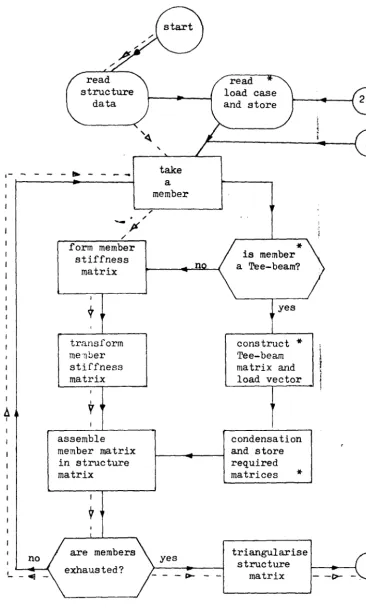
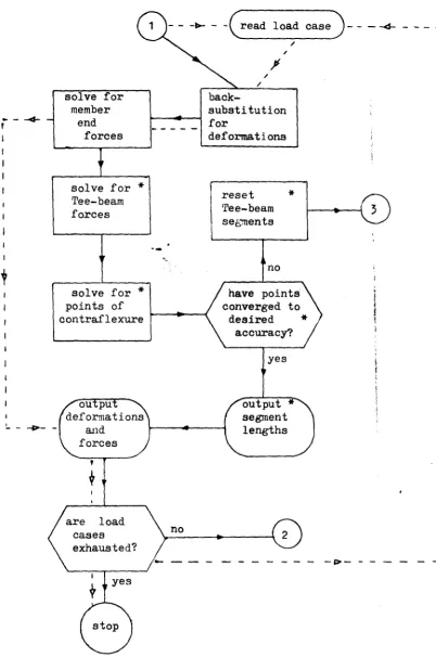
4tenth of the length from each end of the beam. The iteration continues until successive positions of the points of contraflexure have converged to a desired accuracy. The convergence limit of 0.05 ins (0.1 mms) has been built into the program and has proved suitable for general use.

The whole procedure is illustrated by the flowchart given in Fig. 2.5, where the new sections are labelled with an asterisk. An operation manual for potential users has been

issued by the Structural Computation Unit (Manual No.

7

-referring to Manuals Nos. 1 and

5).

Basically there are only two major new additions to the main body of the original program. The first handles the Tee-beam members' stiffness assembly, utilising some of the

procedures listed in Table 2.1. The second is a more independent segment which handles the solution for the points of

oontraflexure. This segment has been given the name INFLEC

TABLE 2.1 Description of new procedures in Tee-beam program. NAME

TB

AVOID

STORELOAD

IFEF

CONDES

POSMEM

PICKUP

SOLVTB

INPUT

section dimensions

member loading

member loading

Tee-beam matrix and load vector segment member

matrix

condensed matrix and load vector

DESCRIPTION

calculates Tee-beam area ru inertia.

constructs structure load , from stored member loads. stores member loads for fu1

use.

calculates the fixed end ef due to member loading for a segment of a Tee-beam for u the total matrix load vecto condensation routine.

TABLE 2.1 continued. NAME

MOMENT

ROOTS

HEINT

PUN OUT

CONY

INPUT

member loading and fixed end forces

moment distribution, member length and

intervals per beam old and new segment

lengths

latest segment lengths

old and new points of contraflexure

DESCRIPTION

forms the bending moment distribution along a Tee-h

finds the number and posit: of zero moment along a Tee·

/ read structure

data

,-

-

- - -

~

- -

-

.-no

,

.

,

- p

/

form member stiffness

matrix

transform me'nber stiffness matrix

,

V

assemble member matrix in structure matrix

are members exhausted?

,

take a member

yes

'--4'1-

- -

-

~

read load case and store

*

is member a Tee-beam?

yes

construct

*

Tee-beam matrix and load vector

condensation and store required matrices

_*

triangularise structure

matrix

[image:35.505.64.431.49.659.2]

... -

-4-,

I

t

~-

-solve for member

end forces

solve for ... Tee-beam forces

solve for ... points of contraflexure

- - -t- - -(read load case) - - 4

-

back-"

I'

substi tution _____ for

deformations

reset

...

Tee-beam seto;ments

".

no have points converged to

desired accuracy?

yes

no

....

-...

- -1>- - -

-Fig. 2.5 continued. Flowchart for Tee-beam program.

[image:36.509.41.444.44.651.2]

It is evident from the flowchart of Fig. 2.5 that a slight re-structuring of the program was necessary. This was

in the positioning of the input load data. Previously the structure stiffness matrix was composed of purely load independent member matrices, but now, with the inclusion of Tee-beams whose

condensed matrix is load dependent, it was necessary to re-position the load input section. This is illustrated by the flowchart which gives both the original and new positions.

The program, already having a user-orientated input system, will handle various types of member loading. This can comprise of any combination of either line, point or moment loads applied at specified locations on a member. Therefore it was required to allow the Tee-beam members to also be loaded in this way.

An

extra facility added to the Tee-beam program was one

to enable the self-weight of a oonorete structure to be included in the frame analysis. This was done internally by specifying a concrete density - 150 lb/cu.ft ( 24 KN/M3 )

- and using the {STOSS cross-section and length to calculate member self-weight. At the input stage it is possible to select those members whose self-weight is to be considered in the analysis.

intervals is set at 100.

As an example, for a Tee-beam member of length 120ins., a typical output could be as

followSI-T-BEAM SEGMENTS

LENGTH :'::N INCHES

MEMBER SEG1

X-SECTION RECT

2 -

3

7.4

SEG2

TEE

105.3

SEG3

RECT

7.4

Fig. 2.6 Example points of contraflexure output.

If only one point exists then the relevant segment will be put to zero length, and in the case where the moment 1s purely hogging - i.e. no points exist - the middle segment will revert to 'RECT' in cross-section. Also output is the number of

iterations taken for all inflection points to have converged to the stated accuracy.

The program is written in 4100 Algol and was developed on an I.C.L. 4130 machine, housed at the University of Warwick. It has been stored in object code on disc ready for use in a batch system process.

of contraflexuxe. Then, a similar frame was simulated for use with the 'ELAN5' program. This was done by introducing new nodes at the points of contraflexure so that different properties could be given for each segment of the beam corresponding to rectangular or tee section as required. The

'ELAN5'

output gave the moment values at the positions of contraflexure and these were expected to be zero if the locations were exaot. The values obtained were indeed very small and it was established that the moments given at determined points of C9ntraflexure were less than

1%

of the smallest end moment of each beam. The results obtained from this test were believed to be satisfactory and well within

any working limits required. The test frame used here is the Bame as that given in the following results section - Example

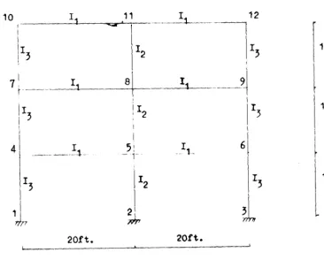
2.5 BJeample l''rame Illustrating the Uee of the Tee-beam PrograJll.

The example chosen is the simple rectangular framed structure shown below in Fig.

2.1.

The actual input and output is given, together with the structure properties. For a specification of the use of the program the reader is referred to Manual

No. 1 issued by the Structural Computation Unit at the University of Warwick.

10 11 11 11 12

oc;ar !

-l,

13 12 10ft.

7

1

I 8 ₁₁

9

r~--

--~--!13 12

13

I

10ft.

4 I

51

I 6

---"1-- -1- - 1-I

13 12 13 10ft.

1 2

3

T

20ft. 20ft.

Fig. 2.1 Example Frame 1.

Member Properties. Breadth Depth Flange Floor Depth In Inches

15 5

11 15 18

[image:40.521.64.430.256.550.2]

,1599~)I) 1500

10 11, _ ... I IfL..,J. J ') ₁₁₂ i

13.45 113.45

. 1

7 8

26 13.45

1750

_1I5J

4

1

1

21

3 (;/;i

Fig. 2.8 Loading Case 1. Dead Load.

Super Load.

Self-weight of membe~.

Unitss Line loads in Ib/ft run, point loads in Kips.

10 12

1044 1750

7

8 9

1750 1044

4

.

1,

5

1 2

lit

Fig. 2.9 Loading Case 2. Dead Load.

Results for the example.

The full computer output is now given together with the moment distribution on the frame for load case 2 in Fig. 2 .10.

[EXAMPLE FRAME] 9,12,15,2,6, IMPERIAL CONCRETE

1;XYR 2,XYR 3,XYR

*

1/4/7/10,3/6/9/12(101-1- . 2/5/8/11(102)

4/5/6;1/8/9,10/11/12(103) 101 )9,12,

102)12,12; 103)15,18;15,5;

*

0,20;40;0;20,40,0,20,40,0,20,40, 0(3,11(3,21(3,31 (3;

*

[DEAD -+SUPER LOAiJ

1-1750 V 4/5,5/6,7/8,8/9, L-1500 V 10/11,11/12;

P -26 V

4,

P -13.45 V 6;7,9,

L

-131

S

1/4;4/7;7/10,3/6,6/9,9/12,

ALL CONVERGED ITERATIONS EQUAL 3

T-BEAM SEGMENTS LENGTHS IN INCHES

MEMBER SEX; 1 SEG2 SEX;3

X-SECTION RECT TEE RECT

4- 5 16.9 176.9 46.2

5- 6 46.2 176.8 17.0

7- 8 20.3 174.4 45.3

8- 9 45.3 174.4 20.3

10- 11 _{12.5 •.} 181.7 45.7

11- ~2 _45.7 181. 7 12.5

CASE 1

DEFLECTIONS IN INCHES ROTATIONS IN RADIANS X 100

J'l'. X-DIRN Y .. DIRN ROTN

1 0.0000 0.0000 0.0000

2 0.0000 0.0000 0.0000

3 0.0000 0.0000 0.0000

4 -0.0014 -0.0530 -0.1155

5 -0.0010 -0.0531 0.0016

6 -0.0006 -0.0453 0.1186

7 -0.0029 -0.0775 -0.1056

8 -0.0029 -0.0844 0.0016

9 -0.0029 -0.0698 0.1088

10 -0.0042 -0.0850 -0.1216

11 -0.0048 -0.0989 0.0016

FORCES KIPS MOMENTS KIPS FT

MEMBER

AXL1

SHR1

MOM1

1-

4

87.47

-1.05

-3.88

4-

7

44.67

-2.42

-12.26

7- 10

14.23

-2.48

-12.09

3-

6

74.93

1.05

3.83

6-

9

44.67

2.42

12.25

9- 12

14.23

2.48

12.09

2-

5

116.72

0.00

-0.03

5-

8

75.80

0.00

-0.00

8-

11

35.65

-0.00

-0.00

4-

5

-1.37

15.36

19.92

5-

6

-1.37

19.63

62.62

7-

8

-0.06

15.67

23.99

8-

₉

_-0.06

_19.33

_60.50

10- 11

2.48

12.~

12.67

11- 12

2.48

17.08

54.18

[DEAD +

SUPER ON ALT.

SPAN~

L

-1750

V

4/5,8/9;

L

-1044

V

5/6;7/8;

L

-1500

V

10/11;11/12,

L

-150 S 2/5;5/8,8/11;

L

-131 S 1/4;4/7;7/10;3/6,6/9;9/12;

*

ALL

CONVERGED

ITERATIONS EQUAL

3

T-BEAM

SffiMENTS

LENGTHS

IN INCHES

MEMBER

SEn1

SEG2

X-SECTION

RECT

TEE

4-

5

17.0

185.1

5-

6

55.8

164.5

7-

8

26.0

160.1

AXL2

SHR2

MOM2

-86.03

1.05

-7.66

-43.36

2.42

-11.90

-12.92

2.48

-12.67

-73.49

-1.05

7.71

-43.36

-2.42

11.90

-12.92

-2.48

12.67

':'115.07

-0.00

0.03

-74.30

-0.00

0.00

-34.15

0.00

0.00

1.37

19.64

-62.66

1.37

15.37

-19.97

0.06

19.33

-60.50

0.06

15.67

-23.99

-2.48

17.08

-54.18

-2.48

12.92

-12.67

sm3

RECT

,:,.~.- .. -.j....:.:. ,.'.,

.,' 1'_'1'::

_r

: J

i

'j

.

. : ::

-.~ ... "

I

i

, J

" I

.j i I'

:"i ':! ,.

' I

"

CASE 2

DEFLECTION;:; IN INCHES ROTATIONS IN RADIANS X 100

JT. X-DIRN Y-DIRN ROTN

1 0.0000 0.0000 0.0000

2 0.0000 0.0000 0.0000

3 0.0000 0.0000 0.0000

4 0.0039 -0.0254 -0.1412

5 0.0042 -0.0454 0.0462

6 0.0046 -0.0254 0.0582

7 0.0045 -0.0389 -0.0506

8 0.0045 -0.0731 -0.0466

9 0.0047 -0.0428 0.1318

10 0.0025 -0.0465 -0.1405

11 0.0020 -0.0876 0.0056

12 0.0012 -0.0504 0.1289

FORCES KIPS MOMElIITS l\ IPS FT

MGMBER AXL1 SH.R1 ,.IOM1 AXL2 SHR2 MOM2

1- 4 '42 .. 31 -1.21 -4.33 -40.87 1.21 -8.95

4- 7 24.89 -2.06 -11.93 -23.58 2.06 -8.67

7- 10 14.35 -2.10 -8.88 -13.04 2.10 -12.'2

3- 6 42.29 0.58 2.25 -40.85 -0.58 4.15

6- 9 31_.99 2.06 8.95 -30.68 -2.06 11.60

9- 12 14.33 2.75 13.82 -13.02 -2.75 13.71

2- 5 99.93 0.63 2.43 -98.28 -0.63 4.45

5-

8 67.24 0.00 2.25 -65.14 -0.00 -2.20

8- 11 35.43 -0.65 -4.51 _-33.93 0.65 -2.01

4- 5 -0.85 15.98 20.88 0.85 19.02 -51.30

5-

6 -1.47 12.02 44.60 1.41 8.86 -13.10

7- 8 -0.04 9.23 17.55 0.04 11.65 -41.81

8- ₉ -0.70 18.66 48.53 0.70 16.34 -25.42

10- 11 2.10 13.04 12.12 -2.10 16.96 -51.25

11- 12 2.75 16.98 53.26 -2.75 13.02 -13.71

Storage Used: 25k. Time: 51 seconds.

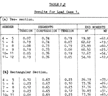
2.6 Some further test results using Tee-beam program.

1. Comparison of the positions of points of contraflexure

and end moments of beams in the given example - ~ig. 2.7 Frame 1 - using: (a) Tee-section beams and

(b) Rectangular section beams.

In the results the three segment lengths are given as a ratio of the total span length &nd the end moments are given in Kips.ft.

TABLE 2--t£

Results for Load Case 1. (a) Tee- section.

MEMBER

!

SEGMENTS END MOMENTS

rENstOlCToMPR:ESstON [ TENSION M1 M2

4 -

5

0.07 0.74 0.19 19.92 -62.66

5 - 6 0.19 0.74 0.07 62.62 -19.97

7 - 8 0.08 0.73 0.19 23.99 -60.50

8 - 9 0.19 0.73 0.08 60.50 -23.99

10- 11 0.05 0.76 0.19 12.67 -54.18

11- 12 0.19 0.76 0.05 54.18 -12.67

~b) Rectangular Section.

4 -

5

0.10 0.61 0.23 26.79 -73.80

5 - 6 0.23 0.67 0.10 73.76 -26.84

7 - 8 0.12 0.65 0.23 31. 76 -70.84

8 - 9 0.23 0.65 0.12 70.83

-31.

76

10- 11 0.08 0.69 0.23 17.36 -65.07

[image:47.511.52.400.213.521.2]

.. J .

:. I

I

.) '2·.

":'l

._ ,1._. .: , . t

' ... i .

<ii'

. --

~.-

.. ". -+1-....

, .. ' . ':r'

.' .: ." _L .. I

, 1

I . . ,. .

l·_ .. ; . . .

t.. ,"

, ....

.... ;-..

~h-l..

'"

~

...

~

..

.. 1 ... )

...

,

I::.~,.l.· I

... 4. ..

2.6 ...

. , I :l :

'1

. . . ; ' 0 , __ .1 ...

! .

~ .. i

. J.. ..

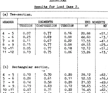
TABLE 2,)

Results for Load Case 2. (a) Tee-section.

-MEMBER SmMENTS END MOMENTS

TENSION COMPRESSION TENSION M1 M2

4

- 5

0.07 0.77 0.16 20.88 -51.30

5 - 6 0.23 0.69 0.08 44.60 -13.10

7 - 8 0.11 0.67 0.22 17.55 -41. 81

8 - 9 0.15 0.77 0.08 48.53 -25.42

10 -11 0.05 0.17 0.18 12.12 _{-51 .25}

11 -12 0.19 0.75 0.06 53.26 -13.71

(b) Rectangular section.

o.4J

4

- 5 0.10 0.70 0.20 28.12 -62.15

5

- 6

0.28 0.61 0.11 52.53 -16.60

7

- 8 0.14 0.58 0.28 21.93 -49.05

8· -

9.

0.19 0.69 0.12 58.65 -33.55

10 -11 0.07 0.71 0.22 16.45 -62.35

11 -12 0.24 0.68 0.08 65.02 -18.35

2. A single example of the variation of Tee-beam end moments with respect to flange width for four different floor

thicknesses i.e. depth of the flange is presented. These results are shown graphically in Fig. 2.11. Only one load case is

considered for the example.

2.7. Comments on the example of Fig. 2.7. and test results.

[image:49.515.38.390.51.351.2]

frame with uniform dead and live loads. Also the iterations taken for the analysis is given as three, but it must be borne in mind that this is not three times the total run time and therefore would not necessarily increase the run time costs by three.

The output of segment lengths enables the positions of curtailment of tensile reinforcement for span and support to be established. If it is desired to find the inflection points for rectangular beam systems, it is only necessary to use Tee-bea:.m with a zero !}oor depth. This is how results given in Section 2.6 were obtained.

From the results given in TABLES 2.2 and 2.3 the size of the compression zone for the Tee-beam case ranges from

0.61

to

0.77

of the span. This agrees reasonably well with the values set in the New Unified Code

6

Where, in Section 3.3.1.2, 'for a continuous beam the distance between the points of zero moment may be taken as 0.7 times the effective span'. A

comparison of results for Tee-beam and rectangular beams shows the increase in the compression zone by use of a Tee-beam and also the reduction in member-end moments, due to the moment attraction of the stiffer Tee-section.

This moment attraction is also shown in Fig. 2.11, where the variation of end moment with flange width is illustrated. However, only the single case, that of a simple frame with

r~8ults. Further investigations have been undertaken,

however, results of these will not be presented in this short report.

2.8 Summary and Conclusions.

'!he Tee-beam program is in a completed user state and has

performed highly efficiently, succeeding in using the condensation technique to advantage. The iteration process and convergence limit have proved adequate for various test frames with irregular loading. However, an improvement to the program would appear possible whereby the bending moment envelope along the beam could be added to the output.

The test results given illustrate the field of investigation which has been undertaken. However, as stated earlier, results of these will not be presented here. Yet the line of researoh appears beneficial and further work in this area would

seem appropriate.

2.9 Referenoes.

1. R. IC. Livesley - 'Matrix Methods of structural Analysis' Pergamon Press, London 1964.

2. P. B. Morioe - 'Linear Structural Analysis' Thames

&

Hudson,

1959.

4. M. F. Rubinstein - 'Matrix Computer Analysis of structures' Prentice-Hall 1966.

5.

G. Bull - 'Computational Methods and Algol' chp. 8,

p. 174-192, Harrap, London 1966.

3.

ORTH~;ONAL SPACE FRAME ANALYSIS.

3.1

Introduction.

A program has been produced to analyse rigid orthogonal space frames, in which the frames are solved elastically by means of a stiffness matrix analysis. The program is not unique, there being many space frame programs in existence. However, this program has been developed only for the testing of other programs.

This is as

followsl-(a) in result testing of development work on more complex computer programs and (b) in comparative result testing of

similar frames analysed by different

pro~ms.

Therefore this program has been restricted to rigid

orthogonal skeletal space frames to facilitate ease of pro~mming and development. Rigid connections are assumed throughout but it would be simple to convert the program for piIllled connections. In a general analysis the transformation from member coordinates to structure coordinates becomes highly complex, especially if a further variable is introduced, that being the orientation of the principal axes to the longitudinal axis of the member. Thus to remove this oomplexity all members in a frame are assumed to be orthogonal in space and have their principal axes parallel to the member axes.

Z(dz)

•

o"---\-~-_ X( dx)

END 1

y.

8---.

x'

ex'

(c) Member-end Forces.

Fig. 3.1. Coordinate systems.

(a) Member coordinate axes and displacements.

(b) Struoture coordinate axes.

'Z

---,_.---y - I -

-END 2

,Z

Mx1

GJ

L

My1

0

~\1 0

Fx1

0

Fy1

0

Fz1

0

:&

Mx2

-GJ

L I

(Y2

0 ~ V1 I

1-Iz2

0

Fx2

0

Fy2

0

Fz2

0

NOTATION

0 0 0 0 0 -GJ 0 0 0 0 0

L

~I 0 0 0

-6EI

0

2EI

0 0 0

6EI

L Y

L1Y

L Y

L~Y

0 ~I 0

6EI

0 0 0

2EI

0

-6EI

0

L z

L2. Z

₁

z

- L1Z

0 0 EA 0 0 0 0 0

-EA

0 0

L

L

0

6EI

0

12EI

0 0 0 bEl 0

-12E1

0

L1.

Z

_L

3Z L~z

--L

3Z

-6EI

0 0 0

1;EI

0

-6EI

0 0 0

-l2EI

L~Y ~Y

"L4.Y

,

---v

y

0 0 0 0 0 GJ 0 0 0 0 0

L

2EI

0 0 0

-6EI

0 ~I 0 0 0

bEl

LY

L2.

Y

LY

L.2.Y

6EI

-6EI

0

2EI

0 0 0 0

k:§I

0 0

1

z

"La.

z

L

Z

1

1z

0 0 -EA 0 0 0 0 0 EA 0 0

L

L

0

-bEl

0

-l2EI

0 0 0

-bEl

0

12EI

0

L

ZZ

--L'z

l.J.z

---V

Z

bEl

0 0 0

-12EI

0

6EI

0 0 0

12EI

L~Y

--L,:r

L2.Y

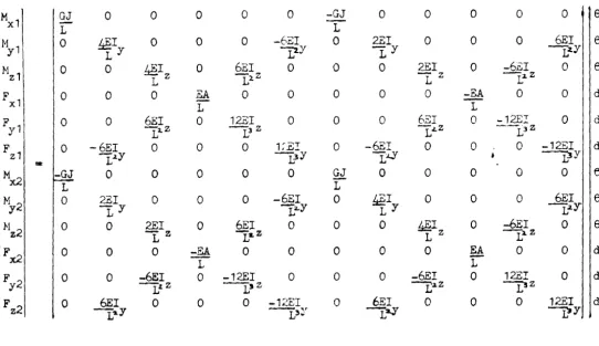
~Y

E and G are the usual elastic moduli, A is the cross sectional area, I , I , J are the sectional properties and L is the member length.

y z

[image:55.776.61.603.38.351.2]

of its type. However, it does enable an elastic analysis of large, three-dimensional, multi-storey frames to be obtained fairly quickly using machines without recourse to backing store i.e. discs or magnetic tapes. But a program of this kind cannot be used to analyse frames incorporating other structural elements, other than beams and columna that is, such as floors and walls. ~r this it is necessary to have a more complex program. However, it may be possible to obtain sufficient information of the required aocuracy using the orthogonal program by ~~oounting for the behaviour of the floor or other structural element in the stiffness of the beam or oolumn elements. It is mainly for this purpose tbat the program has been written.

The program is not thought to be too restrictive, since nowadays a very large number of structures are

orthogonal in nature, for example most multi-storey buildings are of this kind. A quick appraisal of such a building-Is

elastic behaviour in the form of nodal displacements and member end forces can therefore be obtained by the use of this program.

3 • 2 Analysis

In a space frame each node (joint) of the structure will have six degrees of freedom, compared to only three in the plane

size of the resulting structure stiffness matrix will be four times larger th~l that 1n the plane frame oase.

The whole process of constructing the structure stiffness matrix can be swru~ised as

folloWSI-(i) Form the member stiffness matrioes k. (ii) Transform these matrioes to structure

coordinates AkAT •

A is the transformation matrix.

(iii) Add the transformed matrices to form the structure stiffness matrix K.

Or, _{where n is the number of members.}

The equation shown in Fig

3.2

for the member force/displaoement relationship can be rewritten in partitioned form as

=

(3.1)

The matrix A, necessary to transform from member foroes to , structure forces, is of the form

Mx ' T x'x T x'y T x'z 0 0 0

~

My, T _y'x T _y'y T _y'z 0 0 0 M

Y

Mz ' T

•

z'x

T _{z 'y} T

z'z 0 0 0 M z

Fx ' 0 0 0 Tx'x Tx ' y T x'z F x

F_{y '} 0 0 0 T y'x Ty'y T y'z F Y

F 0 0 0 T

where T, is Cos X'QX etc.

_{x x}

Therefore we have

P .. A P

s m (3.2 )

where P is the force veotor and where s relates to the struoture and m to the member.

From the member force/displacement relationship we have

P _m - k d _{m (3.3 )}

where d is the displacement vector.

Using the principal of contragredience the displacement transformation is

(3.4)

Substituting equations (3.3) and

(3.4)

into equation (3.2) we arrive at the result

(3.5)

Using thtl part! tioning as shown in equation (3~ 1) we can expand equation (3.5) as follows

P

1s T 0 k11 k12 TT 0 d1s

=

P_2s 0 T _{k21 k22} 0 TT

_~s

(3.6)

which can be simplified to

P₁ I Tk11 TT Tk12TT d_1s

P2:1

"" T 'rK

22T T

~s

Tk21T _(3.1)

The matrix T is of the form X 0 as shown by Fig. 3.3.

0 X

Taking the term Tk11 T T as typical of the four submatrices

T

'J'k

11'1'T Xk

11aX ~ivin6 as

T T

k 11b ,

Xk_11aX Xk

11bX k11a

where k11

=

k_11d

I

Xk_11cXT Xk_11dX T _k11c

Similarly the other terms in equation (3.7) can be expanded so that the whole transformation process can be

performed on sixteen 3x3 submatrices using just a 3x3 transformation matrix plus its transpose. This is, in fact, the method used

in the program preseIlted here.

A

Simplified flowchart for the program is shown in Fig. 3.6.

3.3 Program.

In the program a procedure called TRANSFORM performs the necessary transformation from member to structure coordinates for each member matrix. Since the member axes are orthogonal to the structure axes the 3x3 transformation matrix will consist of either 0 or +1. This matrix is assembled depending on wnich axis the member's longitudinal axis lies. The member stiffness matrix is previously obtained from the r:.EMBER

procedure.

Having obtained the transformed member stiffness matrix, it is now required to assemble it into the structure stiffness matrix. This is done via the usual node number method. The

6N

i j

I I

I

I

I

I I

i

-

~--- i i - - - - ij

I

j - r- - - - ji - - - - j j

Fig.

3.4

Positions ·of member submatrices in

structure stiffness matrix.

ZERO

TERMS

6N

ZERO

TERMS

STORED

MATRIX

SYMMETRIC

[image:60.492.74.303.30.248.2]

of i i (6x6) is 6x(i-1)+1 and so on for tr!e other elements. Since the structure stiffness matrix is symmetric and banded the actual stored matrix is far smaller than the whole stiffness matrix. 'I'he stored matrix is illustrated in Fig.

3.5,

where the important variable becomes the half bandwidth which is dependent on the nodal conneotivity of the structure.

In

fact it depends on the greatest difference between the numbering of oonnected nodes. If the two nodes concerned are i and j

then the half bandwidth is as

follows.-HEW

=

6x(

IMAX(i-j)

I

+1) (3.8)

the six occurring because of the six nodal variables. It is well to note that careful numbering of a structure can produce an optimisation in size of the half bandwidth which controls the size of the stored matrix.

In the program the assembling of transformed member stiffness matrices is performed by a procedure called STIFMAT which produces the required struoture stiffness matrix in the

'STORED MATRIX' form. The resulting matrix is then triangularised using tile usual Gaussian elimination teohnique.

Restrained variables, i.e. for fixed supports etc., are inoluded via adjustment to the structure stiffness matrix in STI}1~T. The appropriate diagonal element is multiplied by a large number so that its related variable becomes the dominating one.

e.g. to restrain movement of %1

(i.e.

fix %1= 0).

If the first equation of the force/displacement relationship is

a8