Concrete cylindrical shell roofs prestressed within the shell surface

CONCRETE CYLINDRICAL SHELL ROOFS PRESTRESSED WITHIN THE SHELL SURFACE

by A.G. Park

'"

Supervised by J.C. Scrivener

Thes presented by A.G. Park for the degree Doctor of Philosophy

CIVIL ENGINEERING

JUNE 1974

Department of Civil Engineering University of

Christchurch New Zealand

p.6 p.9 p.lO p.48 p.92 p.92 p.102 p.103 p.123 p.124 p.127 p.129 p.145

Fig. 2.1(c): Fig. 2.2: Line 9: Line 19: Line 14: Line 16:

Table of Cable replace and replace Table of Cable

replace Fig. 5.17:

Line 19:

Line 23: Line 3: Line 6:

replace 11m ₁ with "m and "m with "m '

12 12 1

replace "n

l - 8.3%" with "n12 -8.3%" replace "sin(mrjz)" with II

(ll1Tj2) II

replace II

.35dll

with 1/

.35djC l " replace liE " with liE 11

.... D _s replace liE

_"

s D

Data:

Cable Force 1 11410 lb" with "2160 lbll

Cable Force 3 "2160 Ib" with "410 Ib" Data:

Anchorage Force 3 "2160 Ibn with "0 Ibn replace "+ outwardsll

with 11- outwards"

and

replace" inwards" with "+ inwards" The crack referred to is not shown on Fig 5.l4(b). Referring to Fig. 5.14(b) the crack extends one sixth of the arc distance into the shell from the bottom left hand corner of the extrados (as drawn) and from top hand corner of the intrados.

replace "3rd" with "1st"

i

ABSTRACT

Cylindrical shells, constructed of precast concrete

elements prestressed together by means of cables within the

curved surface, are shown to have satisfactory and predictable

behaviour under static load. By careful choice of prestressing

layout, cracking can be delayed until a considerable surface

load has been applied. An existing elastic analysis method

for effects of prestress, based on the D.K.J:. equation, is

adapted to improve its accuracy and efficiency. A method is

given for calculating the effect of the stiffness of the

traverse on the distribution of anchorage force to the shell.

This can be particularly important when the anchorage is

placed close to the shell edge.

Circular cylindrical shell roof models without edge

beams and prestressed within the curved surface with both

straight and draped cables were tested to failure. Four of

the five shells were constructed from precast elements. Strain

and deflection measurements were obtained for all shells and

confirmed the reliability of the analysis method.

A flexural beam type ultimate load analysis is devised

which accurately predicts the ultimate loads of a range of

shells including the model shells tested. This analysis is

developed into a design technique.

Some approximate methods are developed for the working

load analysis of cylindrical shells prestressed within the

ACKNOWLEDGEMENTS

I wish to make grateful acknowledgement for help

received during the course of this project and extend my

thanks to the following people.

Professor H.J. Hopkins, Head of the Civil Engineering

Department, under whose overall guidance this study was made~

Dr. J.C. Scrivener, supervisor for the study, for his

encouragement and constructive guidance throughout this project,

and for his many helpful suggestions during the preparation of

this thesis;

The Technical Staff of 1he Civil Engineering Department

for their assistance in the ~xperimenta1 programme, in

particular Messrs. J.S. Sheard and J.G.C. Van Dyk.

I wish to gratefully acknowledge financial aid from

the New Zealand Portland Cement Association in the form of

the 1970 N.Z.P.C.A. Scho1arshipi and to the University Grants

Committee for experimental equipment and materials under

Research Grant 68/271.

Finally, I wish to thank my wife, Diane, for her const~nt

TABLE OF CONTENTS

Abstract

Acknowledgements

Table of Contents

List of Figures

List of Tables

Notation

1.

INTRODUCTION AND OBJECTIVES

1.1 Introduction

1.2 Historical Background

1.3 Objects of This Research

2.

ELASTIC ANALYSIS

2.1 Range of Applicability of D.K.J. Equation

2.2 Surface Loading

2.2.1 Dead load

2.2.2 Radial load

2.3 Prestressing in Shell Surface

2.3.1 Anchorage force - 1st method

2.3.2 Anchorage force - 2nd method

2.3.3 Line loads - 1st method

2.3.4 Line loads - 2nd method

2.3.5 Convergence of generator line load

technique

2.3.6 Convergence of anchorage loads

2.3.7 Convergence of line loads

2;3.8 Line loads due to a parabolic cable

in a circular curve

2.4 Edge Beams

2.5 Effect of Traverse on the Distribution of

Anchorage Forces

Page

i

ii

iii

viii

xi

xii

1 1

2

3

5 7 8

10

10

10.

11

12

12

14

18

19

21

26

2.5.1 Assumptions 2.5.2 Theory

2.5.3 Determination of

e

2.5.6 Effect of change in

e

3.1 Beam Type Failure 3.1.1 Assumptions

3.1.2 Flexural failure modes

3.1.3 Analysis of "under-reinforced II shell

3.1.4 Accurate determination of f

su

3.1.5 Limitation of maximum steel content to prevent brittle fracture 3.1.6 Limitation of minimum steel content to

prevent steel fracture 3.1.7 Effects of non-prestress steel

3~1.8 Discussion

3.2 Yield Line Mechanism 3.3 Shear Failure

3.4 Buckling

4. DESIGN, CONSTRUCTION AND TESTING OF MODEL SHELLS 4.1 Choice of Model Dimensions

4.2 Design Loading and Stresses 4.3 Choice of Shell Element 4 • 4 Formwork

4.4.1 Shells 1, 2 and 3 4.4.2 Shells 4 and 5 4.5 Reinforcing Steel

4.5.1 1st Shell

4.5.2 Other shell meshes

4.5.3 Traverse meshes 4.6 Prestressing Steel

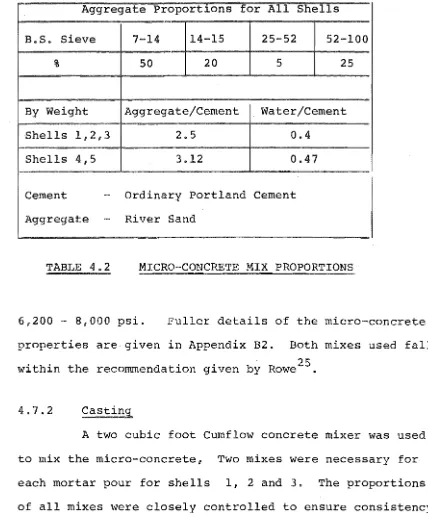
4.7 Concrete Mix and Casting 4.7.1 Concrete Mix

4.7.2 Casting

4.7.3 Curing and stripping 4.7.4 Variation of thickness 4.7.5 Test specimens

4.8 Prestressing System

4.8.1 Solid bearing block

4.8.2 Adjustable bearing block 4.8.3 Load cells

4.8.4 Jack

4.8.5 Anchorages

4.9 Joining, Prestressing and Grouting 4.9.1 Joining

4.9.2 Prestressing 4.9.3 Grouting 4.10 Strain Measurement

4.10.1 Strain gauges 4.10.2 Strain recording 4.11 Deflection Measurement 4.12 Reaction Frame

4.13 Loading Technique 4.14 Testing Procedure

4.15 Evaluation of Young's M.odulus 4.16 Analysis of Strain Data

'"

4.16.1 Prestressing 4.16.2 Surface loading

4.16.3 Symmetry and reliability 4.17 Analysis of Deflection Data

4.17.1 Prestressing 4.17.2 Surface loading

4.17.3 Symmetry and reliability

5. AND THEORETICAL RESULTS

5.1 Elastic Behaviour 5.1.1 Prestressing 5.1.2 Surface loading 5.2 Post Elastic Behaviour

5.2.1 5.2.2 5.2.3 5.2.4 5.2.5 5.2.6 5.2.7 5.2.8

Change in neutral axis position Cracking patterns

Recoverability from overloads Deflections

I

Experimental failure mechanisms o

Comparisons between $k = 30 shells Comparisons between 8'-0" shells

Comparison of shells with and without edge beams

5.3 Ultimate Load Behaviour 5.3.1 1st shell

5.3.2 Shells 2 and 3 5.3.3 4th shell

5.3.4 5th shell

6. APPROXIMATE METHODS FOR THE ELASTIC DESIGN OF PRESTRESSED CYLINDRICAL SHELLS

6.1 Dead and Live Loads 6.2 Anchorage Load

6.2.1 Nl at midspan 6.2.2 Nl near traverse

6.2.3 M2 due to anchorage load 6.3 Draped Cable Loads

6.3.1 Nl due to cable drape 6.3.2 M? due to cable drape

""

6.4 Discussion

vii

7. CONCLUSIONS 161

7.1 Model Tests 161

7.2 Elastic Behaviour 162

7.2.1 Prestressing 162

7.2.2 Surface loading 163

7.2.3 Simplification 164

7.2.4 General ₁₆₄

7.3 Post Elastic Behaviour 165

7.4 Ultimate Load Behaviour 166

7.5 Major Cpnclusions 167

REFERENCES ₁₆₈

APPENDIX A. "D.K.J." COMPUTER PROGRAM _Al

LIST OF FIGURES

Page

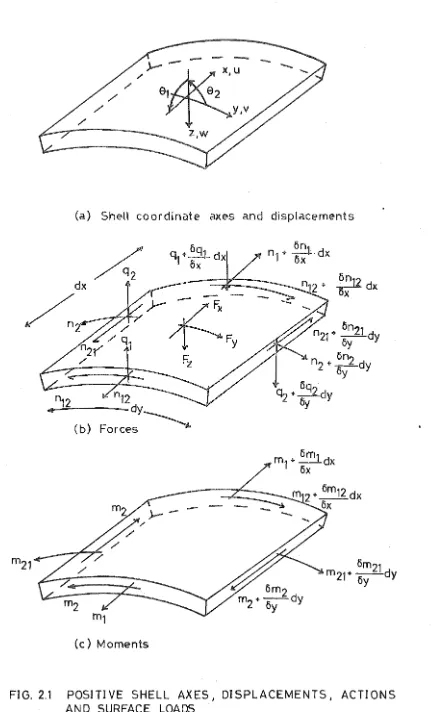
2.1

positive shell axes, displacements, actions

6

and surface loads

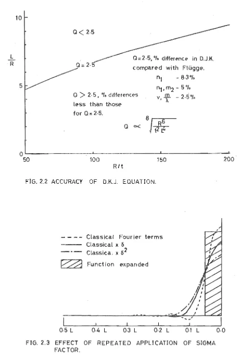
2.2

Accuracy of D.K.J. equation

9

2.3

Effect of repeated application of sigma factor

9

2.4

Effect of Fejer arithmetic mean and

convergence factor

17

2.5

Comparison of triangular and rectangular

pulse expansions

17

2.6

Prestress force distribution using Rish's

method

20

2.7

Comparison of line load expansions

20

2.8

Curvilinear shell coordinate system

20

2.9

Cartesian shell coordinate system

20

2.10 Forces acting on an elemental length of cable

24

2.11

positive edge beam actions and displacements

24

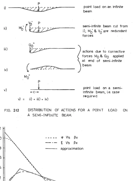
2.12 Distribution of actions for apoint load on a

semi-infinite beam

30

2.13 Variation of

and

with

Sx

30

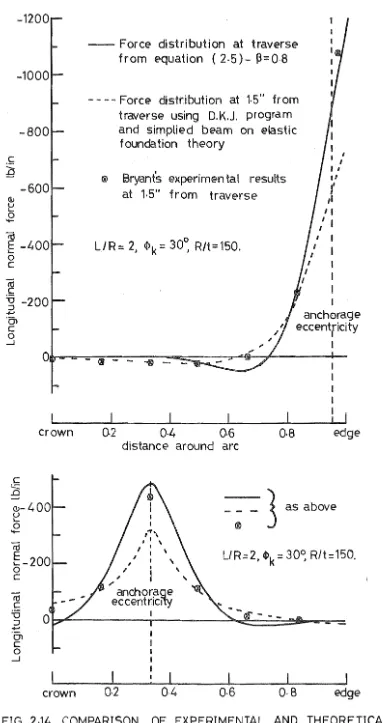
2.14 Comparison of experimental and theoretical Nl

distributions near traverse

32

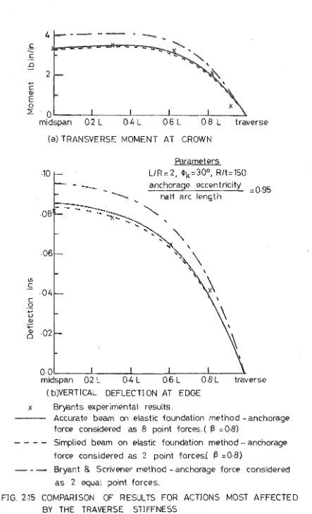
2.15 Comparison of results for actions most affected

by the traverse stiffness

36

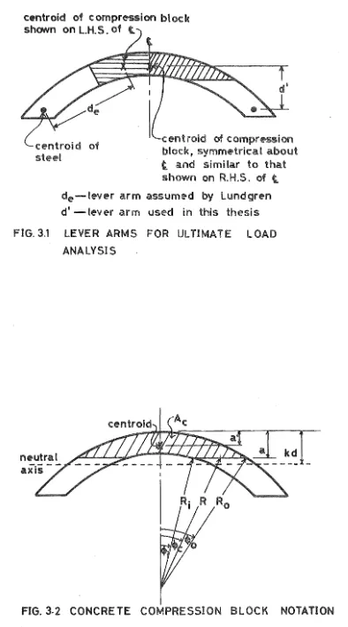
3.1

Lever arms for ultimate load analysis

40

I

3.2

Concrete compression block notation

40

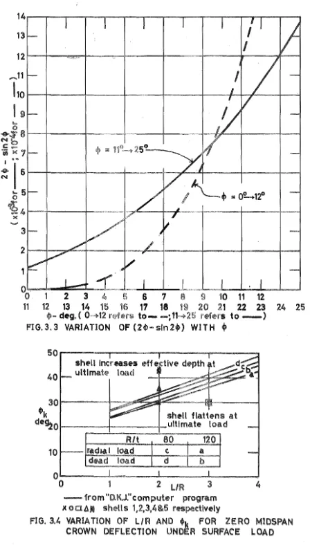
3.3

Variation of

- sin 2

with

45

3.4

Variation of L/R and

~k

for zero midspan crown

deflection under surface load

45

4.1

Assembled shell mould used for shells 1, 2 and

3

65

4.2

Assembled shell mould used for shells 4 and 5

65

4.3

1st shell reinforcing mesh

68

4.4

Typical shell cross-section

68

4.6 4.7 4.8 4.9 4.10 5.1 5.7 5.8

Prestressing system, 2 tor. load cell, and roller support

4th shell prior to testing showing data logger and strain gauge layout

Reaction frame used for shells 1, 2 and Reaction frame used for shells 4 and 5 Loading sequence for shells

3

- Prestressing experimental and theoretical actions and displacements

- Surface loading experimental and theoretical

l.X 75 75 88 88 91

99 -100

5.12 actions and displacements _106-111

5.13

5.14

Midspan variation of longitudinal strain with depth below crown

Crack patterns of failed shells

116 118-119 5.15 Typical surface load versus deflection curve

5.16 Radial deflection across transverse centr~ line 5.17 Horizontal deflections

5.18 Failed 5th shell

5.19 Comparison of deflections for shells with and without edge beams

5.20 Comparison of theoretical moment resistance and experimental failure moment

5.21 Failure mechanism of 5th shell in centre segment 6.1 Accuracy of beam theory results

6.2 Nl at midspan due to unit dead load

121 122 123 123 128 131 135 139 140 6.3 - Midspan Nl due to anchorage load

6.5 142-143

6.6 6.7

6.8 6.9

Variation of midspan Nl with change in R/t Va.riation of M at· crown for change in anchorage eccentricity

M2 ratio envelope

Variation of crown M2 ~t midspan for change in anchorage eccentricity and L/R ratio

6.10 Midspan M2 ratio envelopes

6.11 L

146

147 147 151 152 Variation of crown M2 at 78 from traverse for change in anchorage eccentricity and L/R ratio 153 6.12 M2 ratio envelopes at L/8 from traverse 154 6.13 Variation in M2 distribution for change in R/t 156 6.14 Comparison of results from "D.K.J." program and

A.l comparison of "D.K.J." computer program with results given by Billington

A.2 Comparison of "D.K.J." computer program with results given by Gibson

B.l Load-strain curve for prestressing steel B.2 Load-strain curve for cold drawn wire B.3 Load-strain curve for spot welded wire

results

A2 results

4.1

4.2

4.3

4.4

5.1

6.1

6.2

B.l

B.2

B.3

B.4

B.5

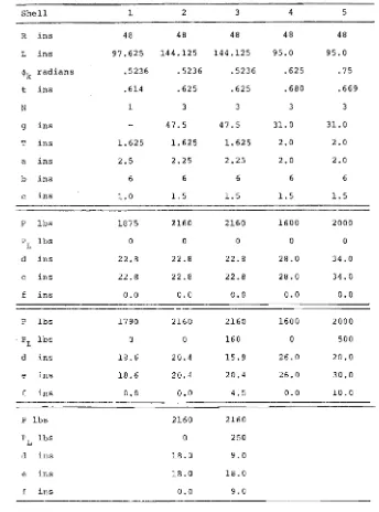
LIST OF TABLES

Dimensions of shells tested

Micro-concrete mix proportions

Typical shell thickness measurements

Typical repeatability of strain measurements

Data used in calculating the theoretical moment resistance of the shells

Influence of traverse on maximum Nl values

Variation of maximum M2 values along shell

due to anchorage

Mortar mix code

Mortar compression tests on

4"

Young's modulus and Poisson's ratio values from strain gauged 4" x 2" cylinders

Tensile tests on 4" x 2" cylinders

Beam flexure test results

xi

60

70

72

93

129

144

149

B6

B7

B8

B8

NOTATION

Each notation is defined where i t first appears in the text. For convenience of reference the more important are listed below:

a constant defining parabola a depth of compression block

a' depth to centroid of compression block

nth Fourier coefficient in the x direction a . nth Fourier coefficient for the ith strip

n~

am mthFourier coefficient in the

y

b b

c

c

c'

c

d

d

d

d'

e

constants of integration for beam on elastic foundation theory i

area of concrete in compression prestressed steel area

non prestressed steel area

concrete area in compression required to balance tendon force T

t breadth of edge beam

effective width of traverse

distance 0f a point force from the end of a semi-infinite beam

parameter describing parabolic cable

coefficient for rectangular stress block depth concrete compressive force

I

anchorage eccentricity as an arc distance from the crown

depth to centroid of prestressing steel from the top of the crown

thickness of traverse vertical lever arm slanted lever arm

f

fc

f I

C

f' S

concrete yield strain

steel strain due to surface loading at ultimate moment

steel strain due to prestressing

steel strain at ultimate moment

nominal steel yield strain

Young's modulus

drape of prestressing cable as an arc length

allowable average concrete compressive stress

concrete cylinder strength

ultimate prestress steel stress

steel stress at ultimate moment

nominal steel yield stress

concrete tensile strength

line loads/unit length in curvilinear coordinates

xiii

F F' F'

x' y' z line loads/unit length in Cartesian coordinates

g parameter describing parabolic cabl~

gi(x) equation of ith strip

h parameter describing parabolic cable

I moment of inertia of shell cross-section

I

z moment of inertia of traverse

k reaction/unit length, for unit deflection in

beam on elastic foundation theory

k positive integer

kd neutral axis depth from top of the crown

L shell span

m positive integer

M general expression for a moment

m

l longitudinal moment/unit length

m

12 twisting moment/unit length

m

M

o

M'

o

Mil o

n

N

Q

r

R R.

].

R

o

t

t

T

corrective moment, which with point force Q is applied to the end of a semi-infinite beam °to remove redundant forces which occur when i t is "cut" from an infinite beam

redundant moment on the end of a semi-infinite beam, when i t is "cut" from an infinite beam

moment due to corrective actions :t.10

ultimate moment positive integer principal normal

longitudinal normal force/unit length shear force/unit length

transverse force/unit length prestressing force

prestressing anchorage force

dimensionless constant used by Boland

and Q o

point force of equal magnitude to redundant shear force Vi

o

positive constant

shell reactions/unit length radius of shell middle surface radius of shell intrados

radius of shell extrados shell thickness

parameter describing parabola unit tangent

tendon force

u displacement in x direction v displacement in y direction

V general expression for shear force V' redundant shear force

o

V"

o shear force due to corrective actions Mo

w radial displacement

and Q o

x,y,z

x,y' ,z'

X,Y,Z

a,S,y

is

e,~,<p,1!! K

]l

shell axes - Cartesian coordinates

shell axes - curvilinear coordinates

surface loads/unit length in x,y,z directions

positive constant?

strain

variables in beam on elastic foundation theory

curvature

coefficient of friction

Poission's ratio

xv

coefficients used in modifying Fourier coefficients

CHAPTER ONE

INTRODUCTION AND OBJECTIVES

1.1 INTRODUCTION

Prestressing offers two main advantages to the designer of cylindrical shells.

First, the large edge beams traditionally used on cylindr-ical shells may be reduced in size, or, if the shell is

prestressed within the curved shell section itself, eliminated completely. This removes the main architectural objection to cylindrical shells. However, by reducing or eliminating the edge beams the inherent stiffness of the shell is reduced. This may lead to excessive cracking, although with careful choice of prestress cable layout, flexural cracking can be avoided until a reasonable load has been applied. For many cases i t is

possible to retard crack appearance until after design working load, thus effectively waterproofing the shell and eliminating the need for any external membrane. A further advantage is that while the section is uncracked, the whole cross-section is effective in resisting deflections.

Secondly, shells can be made of precast elements and joined by means of the prestressing cables. With high labour costs, as in New Zealand, precasting offers considerable advantages that make the use of cylindrical shells a viable economic proposition. Precast elements could be made in a repeatable mould in a

large slope. By the use of top moulds, shells with larger included angles could be constructed more easily than with in situ pouring of shells. Precasting should ensure faster erection on site, thus making construction progress less dependent on weather conditions. Also a reduced amount of skilled site labour would be required.

1.2 STORICAL BACKGROUND

The elastic analysis of circular cylindrical shells, prestressed within the shell surface, has been solved. de Litterl in 1963 and Berndt2 in 1966 described a method for the analysis of circular cylindrical shells with straight prestressing cables and in 1969 Bryant and scrivener3 gave a different method which can be used for both straight and draped cables. Both these techniques use a Fourier type analysis and require the summing of approximately 10 Fourier terms to obtain reliable results. The accuracy of results from these techniques was confirmed by the authors with tests on elastic models.

2

The series of tests carried out by Bryant6,52 on an

were symmetrical. Bryant obtained accurate and repeatable experimental results for his series of tests. He found that his theory accurately predicted the longitudinal stresses away from the traverse and also the frequent changes in sign of the transverse moments. Transverse stresses away from and shear stresses close to the traverse were predicted to within 10%. At the crown, vertical deflections were given to within 3% of experimental results, but near the edges the agreement was between 5% and 25%.

Up to the present time, very few tests have been carried out on concrete cylindrical shells, prestressed within the

4

shell surface. In 1961 Bouma et al reported a series of tests on eleven intermediate length cylindrical shells, one of which was prestressed both in the edge beams and in the shell surface. They found that while prestressing can improve working load behaviour, consideration of the effect of over-loads must be made, particularly with regard to the shell membrane reinforcement, or premature failure may occur.

Scrivener and Megget5 in 1967 carried out what appears to be the only reported test on a single cylindrical shell, pre-stressed within the curved surface and not having edge beams. This shell (L/R

=

=

which were designed to balance the tensile midspan edge stresses due to dead load. Scrivener and Megget found that despite the lack of edge beams, the shell had acceptable deflection and strain levels at normal working loads. The shell was found to recover to near its original state on removal of overloads of up to twice the working load.

1.3 OBJECTS OF THIS RESEARCH

4

was to carry out a systematic series of model tests to obtain reliable data on the behaviour of concrete cylindrical shell roofs, without edge beams, prestressed within the shell

surface. Results from these tests were to be used:

i) To determine whether shells can be designed by an elastic analysis to behave satisfactorily up to design working load.

ii) To ascertain the effect which cracking of the concrete and elongation of the steel has on the behaviour of the shells.

iii) To study the ultimate load behaviour and failure mechanism, and how these are altered with changes

in shell p~rameters.

The second part of the research was to develop an exist-6

ing computer program written by Bryant , so that circular cylindrical shells, with or without edge beams, could be analysed elastically for surface loading and for prestress loading - prestress loading to be either from straight or draped cables in either the edge beam or shell surface.

CHAPTER TWO

ELASTIC ANALYSIS

The elastic shell equation used throughout this thesis

1 k · 7 .

is the commonly used Donne -Karman-Jen lns equatlon:

l2(1-v

where

and E = Young's modulus

R = shell radius t = shell thickness

v

₌

x,y,z

=

u,v,w

=

Shell forces and moments are also defined in Figure 2.1 for future reference.

The D.K.J. equation is derived using Navier's hypothesis, small deflection theory and assuming linear - elastic thin

shell action. In addition the effects of radial shear forces on the shell deflection are ignored.

If the curved ends are assumed to be supported on kni edge supports, with complete rigidity in their own plane, v

=

(a) Shell coordinate axes and displacements

dx

~2

n₁₂ ...,...:.:::..---dy

(b) Forces

~

(c) Moments

6n1 nl + ---+- dx

Ox

standard texts " , • McNamee gives a particularly clear presentation as does Billington9 who shows the deriva-tion of the D.K.J. equaderiva-tion from general shell theory.

Elastic theoretical results used in this thesis were obtained by use of a computer program "D.K.J." described in Appendix A, which is based on the D. K .. J. equation. An indication that the accuracy of the D.K.J. computer program is good is given in Figures A.l and A.2 where results from the "D.K.J." computer program are compared with results

, b 'II' 9 d G'b 22 A b ' f d ' . f glven y B1 1ngton an 1 s o n . r1e escr1pt1on 0

the loading formulations used is given in sections 2.2, 2.3.2, 2.3.4, and 2.4.

2.1 RANGE OF APPLICABILITY OF D.K.J.

Due to the dropping of terms during the formulation of the D.K.J. equation, the range of applicability of the equation is limited. There is, however, some confusion between different texts as to this limit. Billington9 suggests that i t is reasonable to use the D.K.J. equation for short (L/R <}) and intermediate

(~

2~)

A.S.C.El~

11

should be used for larger shells. Hamaswamy recommends that the D.K.J. equation be used for short

(L/R~

shells and that for intermediate (1.6

~

12

8

compared with Flugge theory. Differerices from the Flugge theory are given for the first Fourier term (the second coefficient showing similar trends) and are plotted against a dimensionless constant Q,

nTI a

=

n

=

and hence Q is proportional to

J

As Q is reduced the percentage differences from the Flugge theory increase as does the rate of increase in

differences. The minimum value of Q for which differences are given by Holand is 2.5. These differences are given on Figure 2.2. Figure 2.2 also shows the range of L/R and R/t for which Q is greater than 2.5. In this range

the differences between results using D.K.J. theory and Flugge theory are less than the differences given on Figure

2.2 for Q = 2.5, and should be acceptable for design purposes.

2.2 SURFACE LOADING

In order that the governing differential equation may be solved, loading must be expressed in the form:

x

₌

)

y _{= EY sin yy cos a.x} ) _(2.1)

0

}

Z

=

a.

₌

_L

,

=

L

R

10

5

a<

Q

=

compared with Flugge.

Q>

less than those for Q::: 2·5.

Q 0<

n1 - 8·3°/0

n1 J m2 - 5 %

m '

v -

-

, A

o~---~~---~---~

50 100 150 200'

Rit

FIG. 2.2 ACCURACY OF D.K.J. EQUATION.

0·5 L

Classical Fourier terms Classical x 6

Classical x 62

Funct ion expanded

0·4 L 0·3 L 0·2 L 0·1 L

FIG. 2.3 EFFECT OF REPEATED APPLICATION OF SIGMA FACTOR.

10

2.2.1 Load

At any position on the shell cross-section, distance y around the arc from the crown, the dead load force P per unit area can be resolved into two components Y and Z where:

Y

=

This is the same form as equations (2.1) if ¢ == Y/ R := YY . In order that uniform dead load is obtained along the shell Y, Z must be expressed in the form (4P/nn) sin (nn/z) . Hence for dead load:

x

Y ₌₌

_-

r;-n R

Z ₌₌

-

_r;-

n R

2.2.2 Radial Load

At all points on the shell for a uniform radial pressure P , X := Y == 0 and Z == P . In a similar manner to dead load:

Z == 4p

L1.

n n

T

r;-2.3 PRESTRESSING IN SHELL SURFACE

cos YY _ 1

A number of methods, some approximate, have been

proposed for the analysis of cylindrical shells prestressed within the shell surface. Approximate methods where the line loads (forces from friction and cable drape) have been replaced by equivalent loads along the shell edge have been

d 1 4 14 h 15 d ' 16

favourable circumstances, their overall accuracy is

doubtful and the use of a more accurate method is preferable. For the more accurate methods, described in the following sections, there are two fundamentally different techniques for representing both the anchorage force and the line loads.

2.3.1 Anchorage Force - 1st Method

Berndt2 and de sitterl solve the problem of the . anchorage force on the end of the shell in two steps.

In the first stage the shell is considered as being simply supported along the straight edges and the anchorage force is expanded along the curved end as a Fourier series P(y) :

P(y) == - - cos a 2p d cos a y

R¢K n n

where a

n n == 0,1,2 . . .

d == anchorage eccentricity The boundary conditions are:

i) Curved ends

w=v=m =0 ₁ n

l = P(y) ii) Straight edges

m ₂ = n ₂ == 0

The second stage consists of removing the unwanted actions, n

12 and r 2 ' along the straight edges by a complementary function solution with the shell simply supported on the curved ends.

2.3.2 Anchorage Force - 2nd Method

12

at the curved ends and that the anchorage force is introduced to the shell as a shear force over a short longitudinal

length of the shell adjacent to the traverse. The analysis technique is a particular case of that used for draped cables described in Section 2.3.4.

2.3.3 Line Loads - 1st Method 2

The method used by Berndt and also investigated

, 6

by Bryant is to substitute the line loads by statically equivalent surface loads which are then developed as a double Fourier series:

sin Ct x cos

ex x

sin myy cos myy

n,rn are odd integers

Berndt reports that he found good agreement between model test results and results using his method of analysis. ' However, Bryant found that the above method did not give satisfactory convergence for some shell actions and so he developed the following method.

2.3.4 Line Loads - 2nd Method

The method described in this section is largely a summary of a paper by Bryant and scrivener3.

First the shell is divided up into a number of transverse strips of width L/ 2m , m being an integer, throughout which the line load intensities are considered constant. A number of equally spaced shell generators are then considered along the cable profile and the line loads divided between them. For each transverse strip the line load is divided between

generators the line load components F , F , F

z are replaced

x y

by the actions The anchorage load is consid-ered to be a shear load (n

12) spread into the shell along

two generators adjacent to the anchorage and treated similarly to the line loads.

These actions, n

12, n2, r 2, are then expanded as a Fourier series along each generator in order that a Levy type solution may be applied. If gi (x) is the equation along a generator for a line load component (value f (x.) )

~

of the ith transverse strip.

n1TX

1 n1TX.

where a sin n1T 1

ni

=

-

=

~

=

Then from the sum of all strips

m _{8 cos n1TX}

f(x) = E gi (x)

=

-

sin i';"l 1T n n

m

f (xi) where a = a

ni n == 1,3,5 n E

i=l

For each Fourier term the analysis is carried out as follows:

i) The shell is considered as a complete tube and

solved for each pair of symmetrical (one from each side of the centreline) generators. This is done by assuming that the loaded generators divide the tube into two shells and hence the generator loads can be considered as edge loads at the junctions of the

required points anywhere on the tube.

ii) All the complete tube solutions are then added

together and the required shell "cut" from the

tube, unwanted edge sections being removed by an

ordinary complementary function solution.

Bryant and scrivener3 have compared results obtained

14

by the above generator line-load method with experimental

results obtained for a number of cable layouts on a prestressed

aluminium model shell. Good correlation was obtained.

2.3.5 Convergence of Generator Line Load Technique

From the results of trial runs, Bryant and

Scrivener found that if 10 Fourier terms (n==1,3 ••• 19) were

summed for an anchorage load spread 0.05L into the shell

along two closely spaced gen~rators, a reasonable

approxi-mation of the anchorage load was obtained. For draped cables

they found that a generator spacing of R<Pk/6, m == 20 transverse

strips and 6 Fourier terms were required to give the same order

of accuracy as that obtained for the anchorage load.

An attempt, as described below, was made by the present

author to improve the convergence of the solution by using

different methods for modifying the classical Fourier coe

icients. However it was found that little improvement in

the convergence could be obtained from that using the

param-eters and method suggested by Bryant and Scrivener. The

greatest variation between methods occurred in the vicinity

of the cable near the traverse. Away from this area there

was negligible difference between many of the methods. For

the anchorage force a triangular shear pulse was considered

and Scrivener. Expressions for the rectangular and triangular pulses are:

Rf!'ctangular pulse'

_I

..

,

•

a

I

a

~-~J."'"

t E - - - L 12

---'lllOt

-Llr~ ~

Triangular pUI se

I

t;~

______________

~;;,_a~~,~,s.

ILl2

-Llr~

f(x)

n=l, 3 •••

and for anchorage force p

f(x_{i )} ==

L/R

8 r f (x. ) 1

f (x) = 1 cos n1T (1 ) sl'n n1T

2

2"

- -

(n1T) r

n

=

Three methods of modifying the Fourier coefficients were tried. All of these methods distort the original function and hence a balance must be reached between this distortion and the reduction in Gibbs oscillations. The methods used were:

Sigma Factor This method is described by Lanczos 17 and involves multiplying the Fourier coefficients by a factor ok'

sin klT/n

°

=

. k klT/n

where n == the number of Fourier terms to be considered k = kth Fourier term.

The effect of multiplying by the sigma factors is essentially to replace a function f(x) by f(x) where

f (x) =

2n~ f,~f

+

This new function smooths the original function by taking

at each point the arithmetic mean between the limits

Multiplication by the sigma factors can be repeated on the

new function, i.e. if the sigma factors were to be applied

16

twice, the classical Fourier coefficients would be multiplied

by

At each step the convergence becomes stronger, but

the operation of local smoothing distorts the function and

stronger convergence is obtained, not to the original function

but to a modified function.

The reduction in Gibbs

oscilla-tions and distortion of the function is shown in Figure 2.3

for a rectangular anchorage block, where it can be seen that

for

cr~

the slope of the graph is less than cr

_k

•

As a steep

slope is required in order that the line load is applied as

near the end of the shell as possible, any use of the sigma

factor beyond cr

_k

is not advisable.

Fejer Arithmetic Mean

Again described by Lanczos

,

this method involves taking the arithmetic mean of the partial

sums of the Fourier coefficients up to the nth term.

If S

=

o 0

cr

n

=

Lim. cr

f (x)

n

S 'i'

• . • _n-"' 1 n

This is equivalent to multiplying each Fourier term by Pk(n)

where Pk(n)

=

(1 -

~)

The summation converges to f(x) from below as shown in

Figure 2.4, for a rectangular anchorage pulse.

Figure 2.4

also shows that the Gibbs oscillations can sometimes be

- - - - Classical Fourier terms _ - - F ejer ari t hmet ic mean ---. - Convergence factor

Function expanded

-

--0·5 L 0·4 0·3 0·2

0·1

FIG.2.4 EFFECT OF FEJER ARITHMETIC MEAN AND

CONVER~ENCE FACTOR.

0·5 L

Classical Fourier terms Function expanded

Classical x (j factor Funct ion expanded

0·4 L 0·3 L t:)·2 L 0·1 L

0·0

0·0

FIG.2.5 COMPARISON OF TRIANGULAR AND RECTANGULAR

18

Convergence Factor This method is presented by Baryl8.

Each Fourier term is multiplied by l/loge k except when

k = 0 or 1. Figure 2.4 shows that although the convergence

factors eliminate the Gibbs oscillations, the slope at the

discontinuity is less than that given by the other methods.

2.3.6 ~nvergence of Anchorage Loads

As the distance over which the anchorage pulse is

assumed to act is decreased, the rate of convergence of the

Fourier series decreases.

The best method of applying the anchorage force using

a rectangular pulse is to use the classical Fourier

coeff-icientsand a pulse spread O.05L into the shell. This is

the same as suggested by Bryant and Scrivener. For a

triang-ular pulse the best method is to use the CJ

k x classical

Fourier coefficients, spreading the pulse again 0.05L into

the shell. These two expansions are compared in Figure 2.5.

There is little difference between the two expansions although

CJ

k x Classical Fourier coefficients would appear to be better

as with this expansion the total anchorage force is applied

to the shell closer to the traverse. Computer results from

the D.K.J. program show negligible difference between the

two expansions, except near the anchorage line close to the

traverse.

The above discussion is for 10 Fourier terms; however,

similar behaviour occurs for different numbers of terms. If

less than IO-terms are used the Gibbs oscillations will be

greater and the slope at the discontinuity less. The choice

of method would depend on whether the force is to be applied

near the end of the shell or whether the oscillations are to

' h

t'

'th th

t

.

f

d

b

R1S

, 1n connec 10n W1

e pres ress1ng 0

e ge earns,

has suggested a method for reducing the number of Fourier

terms required.

The prestressing force is applied as a

triangular shear pulse spread O.2SL into the shell, which

gives an almost perfect parabolic distribution after 4 Fourier

terms as shown in Figure 2.6.

Using a simplified form of.the characteristic equation

an edge correction is then made to return the prestress force

to the corners of the shell by applying corrective shear forces

to both the edge beam and shell edge.

The corrective shear

forces increase linearly to the traverses, from zero at the

quarter points, and their effect on the prestress force

distribution in the shell is shown in Figure 2.6.

It would appear that this technique could also be used

for prestressing in the shell surface if the generator line

load method is used.

However, the technique was not tried

out as it was felt it would give no more accuracy than the

present D.K.J. computer program and that a reduction in the

number of Fourier terms summed would make only a slight

difference in computation time required.

2.3.7

Convergence of Line Loads

Similar trends between different Fourier expansions

occur for line loads as for the anchorage loads.

The best

methods are the classical Fourier coefficients used by Bryant

and Scrivener or 0kx classical Fourier coefficients.

These

are compared in Figure 2.7 for a line load at L/4 , similar

trends occurring for line loads at other positions along the

shell length.

0·5 L 0·25 L 0·0

20

VIZ

I

II 1 II

Prestress force distribution in shell

rue

Prestress force distribution in shell due to cor r ective shear force.

FIG. 2·6 PRESTRESS FORCE DISTRIBUTION USING RISH'S METHOD.

VZ/J

Function expanded

- - - Classical Fourier terms

- - - Classical x c1 fact or .

...

..

-

...

..

....

..

_..

_,

..

-

,

-

_I

_I

0·5 L 0·4 L 0-3 L 0·2 L 0·1 L 0·0

FIG. 2·7 COMPARISON OF LINE LOAD EXPANSIONS .

... x -

0

"

"v

_{... -}

-_..L

₂

FIG. 2·8 CURVIUt\IEAR SHELL COORDINA TE SYSTEM

z'

coefficients) or whether a better convergence of the line

load, but spread

a greater length of shell, is desired.

However, as the effect of line loads is of a secondary order

compared with the anchorage load, the difference between the

effects from the two expansions will be small, except close

to the line load.

2.3.8

Line Loads Due to a Parabolic Cable In A Circular Curve

The line loads derived in this section occur when a

cylindrical shell of constant radius is prestressed with a

cable which is parabolic in the developed shell surface.

Using the curvilinear coordinate system of Figure

the parametric equations of the parabola in the developed

shell surface can be written:

t

x

=

_2a

Y

=

-=

-2

ax

where

t 2

4a

e

=

a

=

d+f

4f

L2 •

Bryant and Scrivener have used curvilinear coordinates to

calculate the line loads due to a parabolic cable in a

circular curve, however it is simplerto use the Cartesian

coordinates of Figure 2.9 and thus the parametric equations

become:

x

=

_2a

y'

=

Rsin$

where $

=

¥..

R 2

4ae -

4aR

Z I =

-R cos $

=

A point on the cable can be defined by a position vector

r(t)

(2

t

a ' Rsin$, - Rcos$),

therefore

dr

1

and

2

r 1

----,;r = -

(0, -coscp

+

c sin

-sin

-coscp ) ,

dt"

2a

unit Tangent - T

Kreyszig

20

(pp271) defines the

unit tangent, T , as

dr

T

₌

dt

I~I

1

_{(1, -tcoscp, - t sincp )}

2a

11

+

t

2

1

_{(1, -tcos<jl}

_{- t sincp ) •}

=

,

.1

₁

₊

_t

2

Curvature - K

dT

dT

dt

KN

ds

=

dt

d'S

th~refore

KN

=

Now

therefore

I

ddTSI

N

Principal Normal

K

=

Curvature

K =

2a

I

t 2C2

c 2

1

(1+t 2

Principal Normal -

dT

ds

IdTI

ds

=

2

~

2

{-t,-[cos<p -

c

sin<p - t

2

c sin<p],

(l+t ) (t c +0' +1)

2 ,.

sin<p + c cos <p+ t c cos <p ] }

Line Loads in

Coordinates

Consider a

small length of cable Os

shown in Figure 2.10.

oe

-

os

=

R s

The resultant force due to the cable curvature is

poe

and

it is directed along the principal normal.

poe

This can be written as

force/unit length in the

direction

Similarly, forces directed along the unit tangent/unit'

length in the

direction

ds

=

«(Jj

+

ax '

where

w

=

wobble factor

Now

therefore

Also

therefore

=

force/unit length to bodily move the cable.

ds

dx =

ds

dt

dt

2a

Ox

dt

ax

and

₌

_2a

ds =

,Adx) 2+

(~)2

+(dz

2

dt.

at

a t

dt

==

1-

'1'+t

2

/

p

I I

I

____ centre of curvature

~ for

oS

1\

I \

109\

~\

\

\

\ \

55

-\

\

P

FIG. 2·10 FORCES ACTING ON AN ELEMENTAL LENGTH OF CABLE.

/

I I

: I

; - - 1

-" I

(a) Forces and moments

Wb

(b) Displacements

poe

the curvature force

PK

ds

ag

dx:=

h2

and tangential force

and h

/1 + t

2

(w+v PK)

~

+

a3g

Resolving these forces in the x, y',

z'

directions

Fx

2 a tP +

+

~

P

h

3

}:1

F '

= -

a .

(cos

cp-

c sin<p- t

c 2 sin

+~

cos

y h

F

2aP (sin<p+ccos<p+t

c·

cos<p)

~vp)tsin<P

z

h3

The forces F,

Line Loads in x, y,

Coordinates

F' F'

y ' Z

can nowbe resolved into components along the curvilinear

coordinate directions.

F

F

-

2 atP

P +

₊

~

h

3

x

x

h

F

_F

_cos

cp

+F' sin

Y

z

=:

2a P

-

+ 2 a g

P) t

t;!

h

3

F

_z

F z' cos

- F ' sin

-2acP

_h

-y

These are the same forces obtained by Bryant and Scrivener

except that in their paper they have'mistakenly multiplied the

forces by h .

At the traverse, the anchorage force component in the x

direction is

=

Anchorage force

26

2.4 EDGE BEAMS

The effect of edge beams on a cylindrical shell can be

considered by means of a complementary function solution9,lO.

In order to obtain compatibility with the shell edge,

all loading on the edge beam must also be expanded as Fourier

series. For a prestress cable draped parabolically in the

edge beam, the loading on the edge beam can be expressed in

the form,

P_B

4 P_A

I n'ITx

=

'IT _{n n}

MB

4 P_{A 1 n'ITx}

::: _{- - E cos}

r:;-'IT _{n n}

VB

32 P_A f _{1 n'ITx}

::: _E

-

n L

n

where P

A ::: prestress anchorage force acting on edge beam

P

B ::: normal force along edge beam due to prestressing

MB ::: _{moment along edge beam due to prestressing}

e

=

VB ::: _{shear force along edge beam due to prestressing}

f ::: cable drape.

positive actions and displacements at the centroid of

the edge beam are shown in Figure 2.11. The solution requires

that compatibility of displacements and actions along the

shell-edge beam junction be maintained. In order to do this, a

translation matrix is used to obtain the actions and

displace-ments of the edge beam at the junction. A rotation matrix is

then applied to obtain the actions and displacements in the

same coordinate system as that of the shell, at the shell

2.5 EFFECT OF TRAVERSE ON THE DISTRIBUTION OF ANCHORAGE FORCES

The distribution of prestress anchorage force along the

end of the shell will depend on the properties of the traverse.

For instance if a traverse is made stiffer, the forces will be

spread into the shell over a greater arc length. Hence rather

than assuming that the anchorage force is spread equally down

two generators at some arbitrary distance close to the

anchor-age, an analysis technique is presented below which takes into

account the effect of the traverse stiffness on the

distribu-tion of anchorage forces to the shell. The effect of the

traverse is particularly important when the cable is near the

edge of the shell as the transverse moment and radial

deflec-tion may be significantly affected.

The following analysis technique, based on the theory

of beams on elastic foundations, is a means of calculating

the distribution of anchorage prestress force, including the

effect of the traverse (beam) on the end of the shell (elastic

foundation). In Section 2.5.7 the method is shown to give

good correlation with experimental results.

2.5.1 Assumptions

The basic assumptions made are that both in-plane

shear force between the traverse and the shell, and curvature

of the shell are neglected. The first approximation is not

serious as the in-plane shear force between shell and traverse

due to prestressing is generally small, and the second

approx-imation is reasonable if the anchorage force distribution is

spread over a relatively short arc length, as would occur in a

majority of shells.

2.5.2 Theory

The theory for beams on elastic foundations has been

For a beam on an elastic foundation, the reaction from

the foundation/unit length

ky

W

where y

deflection of beam and foundation

k

reaction/unit length when y

.

Now for a beam

d

_y

dx

therefore

The general solution is

y == eSx(A cos Sx +

sin Sx)

+e-Sx(CcosSx+Dsin Sx)

.4/~

where S

Z

Considering the case of an infinite beam with a single

point load,

the boundary conditions are:

i)

At points infinite from the load, y

2B

therefore A

and y

e -Sx (C cos S x + D sin S x)

ii)

At point where the load is applied, i. e.

x ==

~~

therefore C::::; D and y

C -Sx (cos a x + sin S x)

Now for

_x

_dx3

3

and shear force, Vx==O

-EIZ(~)

==

dx

p

- '2 •

Therefore

C

BS3

pa

-ax

_{a x + sin Sx)}

y

_{- - e}

_(cos

2k

M == -EI

d

2

_y

dx

2

and the moment

P

-Sx

.

==

-n

e

(sl.n

x - cos S x) •

Using the notation

e

-Sx

('1os ax + sin ax)

e =

e

-j3x

cos j3x

~

=

e

-j3x

sin j3x

y

Pj3

_cj>(ex)

P

M

413

_'¥(ex)

(2.2)

....

V

_'2

P

a (ex)

Considering the case of a moment,

Mo' being applied

at the end of a semi-infinite beam it can be shown that:

y

~

(ex)

M

_{Moa(ex )}

....

(2.3)

)

)

V

-6 Mo cj> (ex)

Using the above two cases, the distribution of y, M,

can be found for a point load on a beam of semi-infinite

length, as shown diagrammatically in Figure

Referring

to Figure

the redundant forces M

and

at the

o

end of a semi-infinite beam when it is "cut" from an infinite

beam, can be found from equation

Le.

M'

o

P

=413

and

::::

~

[a

(ec)]

From equations (2.2) and (2.3), the actions

and M

due to corrective forces

and

o

applied at the end of

the semi-infinite beam can be found.

Le.

MA

M

o

_and

o

Hence by equating

o

and

o

=

be shown that

Q

o = P (2 [8

Uk)]

+

'¥ (ec) )

Mo

-~

('¥(j3c)

+

8 (ec)

) ) )

••• (2.4)

1-2

1.0

·8

IP

or

·6

_.4

.2

0·0

iii)

IV)

(

M

o

v)

p

p

..-c-point load on an infinite beam·

semi-infinite beam cut from

j), MO' & Vo are redundant forces

actions due to corrective forces MO

&

beam

30

v) = ii) + iii) + iv)

pOint load on a semi-infinite beam, i. e. case required

FIG.

2·12

DlSTRIBU TION OF ACTION;S FOR A POIN T

LOAD

ON

A SEMI-INFINITE BEAM.·

....

-

-

-

g

approximation

"".... ...

_

__

-I I I I

J

0·0

1·0

2·0

3-0

4·0

5·0

px

Thus for a point load distance c from the end of a

semi-infinite beam, x-c W =-ky

=

Q

f3

+

+

{<Ii

••... (2.5)

i.e.

are plotted in Figure 2.13 for variation in S x.

The distance from a point force over which bending occurs

is given by Timoshenko as

'is,

deform-ations and forces a value of

~S

means that abeam may be considered semi-infinite if part of

it lies further than

~f3

force is applied to a beam at a distance greater than

~S

from both ends of the beam (i.e. an "infinite" beam) the last

two terms of equation (2.5) can be ignored.

To calculate the distribution of prestress anchorage

force from the traverse (beam) to the shell (elastic foundation),

equation (2.5) is used. Typical force distributions are shown

in Figure 2.14, both for an anchorage force close to and away

from the edge. When the anchorage is near the edge the

maxi-mum force/unit arc length is greater than when the anchorage

is away from the edge. Also the maximum force/unit arc

length occurs at the edge of the shell and not at the

anchor-age.

The technique can be used in a generator - line load

type computer program by summing the force distribution over

discrete arc lengths of the shell. The resultant forces are

then applied to the shell as point loads at the centroids

-800

.~

-g

...

1...-200

en

- Force distribution at traverse from equation (2.5) - ~: 0·8

- - - - Force distribution at

1·5"

foundation theory

® Bryant's experimen tal results

at

1.5"

LlR:2,

4>k:::30~

I

I I

I I I

I I

! I

t

,1

I I

I I I I I I anchorage eccentricity I

0·2 0·4 0.6 0·8 edge distance around arc

,

'"

,

I ,

anchoraqe eccentricity

I

0·2

0.4

-; -3

LlR=2, 4>k:::

-

..

0·6 0·8 edge

FIG.

2.5.3 Determination of

S

E

t

=

Assuming the shell acts as a column,

P

k

=

tE s

Es ~ Young's modulus of shell I

z

=

bd3

I

z

=

lC2

=

b = effective width of traverse.

40

By considering the A.C.!. recommendations for the effective widths of L-beams, b has been defined by:

Hence

and if

b ~ 6 x d ~ 1

16

. .

~

E

=

t s

J

=

L

.•. (2.6)

2.5.4 Summary of Method

i) Calculate

S

o from equation (2.4)

2.5.5 Simplification

The above method involves the summing of

non-linear relationships in order to find the distribution of

prestress force around the arc on the end of the shell.

The following procedure, which has been found to give

satisfactory results, is suggested in order to simplify

calculations.

i) Calculate f3 from equation (2.6).

ii) Calculate Mo and Q _o from equation (2.4).

34

iii) Approximate ~ and ~ curves to the triangular shapes

shown in Figure 2.13.

iv) Sum the forces on each side of the anchorage

2.5.6

separately, and calculate the centroid of each

force block.

v) Use the two forces calculated, acting at their

respective centroids, to find the effect of the

prestress anchorage force on the shell.

When the anchorage is further than 1.9 from f3

the shell edge, the

p

two equal forces,

2

the anchorage.

above simplification gives

d · t f 1.9 f

, at a 1S ance 0

±:nr

Effect of Change in f3

If the relative stiffness of a traverse is increased,

f3 will decrease. Except near the edge, the only effect that

a decrease in f3 will have is to spread the anchorage force

over a larger arc length, the distribution curve remaining

a similar shape. However, near the edge, as well as

spread-ing over a larger distance, the curve will change shape.