warwick.ac.uk/lib-publications
Original citation:
Hulusic, Vedad, Debattista, Kurt, Valenzise, Giuseppe and Dufaux, Frédéric. (2016) A model
of perceived dynamic range for HDR images. Signal Processing: Image Communication
Permanent WRAP URL:
http://wrap.warwick.ac.uk/84260
Copyright and reuse:
The Warwick Research Archive Portal (WRAP) makes this work by researchers of the
University of Warwick available open access under the following conditions. Copyright ©
and all moral rights to the version of the paper presented here belong to the individual
author(s) and/or other copyright owners. To the extent reasonable and practicable the
material made available in WRAP has been checked for eligibility before being made
available.
Copies of full items can be used for personal research or study, educational, or not-for-profit
purposes without prior permission or charge. Provided that the authors, title and full
bibliographic details are credited, a hyperlink and/or URL is given for the original metadata
page and the content is not changed in any way.
Publisher’s statement:
© 2016, Elsevier. Licensed under the Creative Commons
Attribution-NonCommercial-NoDerivatives 4.0 International http://creativecommons.org/licenses/by-nc-nd/4.0/
A note on versions:
The version presented here may differ from the published version or, version of record, if
you wish to cite this item you are advised to consult the publisher’s version. Please see the
‘permanent WRAP URL’ above for details on accessing the published version and note that
access may require a subscription.
A Model of Perceived Dynamic Range for HDR Images
Vedad Hulusica,∗, Kurt Debattistac, Giuseppe Valenziseb, Fr´ed´eric Dufauxb
aLTCI, CNRS, T´el´ecom ParisTech, Universit´e Paris-Saclay, 46 Rue Barrault, 75013, Paris, France
bLaboratoire des Signaux et Syst`emes (L2S, UMR 8506), CNRS - CentraleSup´elec - Universit´e Paris-Sud, 91192 Gif-sur-Yvette, France cWMG, University of Warwick, CV4 7AL, Coventry, UK
Abstract
For High Dynamic Range (HDR) content, the dynamic range of an image is an important characteristic in algorithm design and validation, analysis of aesthetic attributes and content selection. Traditionally, it has been computed as the ratio between the maximum and minimum pixel luminance, a purely objective measure; however, the human visual system’s perception of dynamic range is more complex and has been largely neglected in the literature. In this paper, a new methodology for measuring perceived dynamic range (PDR) of chromatic and achromatic HDR images is proposed. PDR can benefit HDR in a number of ways: for evaluating inverse tone mapping operators and HDR compression methods; aesthetically; or as a parameter for content selection in perceptual studies. A subjective study was conducted on a data set of 36 chromatic and achromatic HDR images. Results showed a strong agreement across participants’ allocated scores. In addition, a high correlation between ratings of the chromatic and achromatic stimuli was found. Based on the results from a pilot study, five objective measures (pixel-based dynamic range, image key, area of bright regions, contrast and colorfulness) were selected as candidates for a PDR predictor model; two of which have been found to be significant contributors to the model. Our analyses show that this model performs better than individual metrics for both achromatic and chromatic stimuli.
Keywords: High Dynamic Range, Perceived Dynamic Range, Subjective Evaluation, Predictor Model
1. Introduction
High dynamic range (HDR) technology [1, 2] enables the capture, storage, transmission and display of the full range of real-world lighting and colors, with a significant increase in pre-cision when compared to traditional low dynamic range (LDR) imaging. One of HDR’s main features is its ability to reproduce very bright and very dark portions of a scene concurrently. The span between these extrema in the brightness scale is commonly referred to as thedynamic rangeof a picture.
The dynamic range of image or video content is frequently reported by many HDR applications. It is typically computed as the ratio between the maximum and minimum pixel lumi-nance of an image, which will be referred to aspixel-based dy-namic range (DR) in this paper. Such a computation can be bi-ased due to image noise or singularities, such as isolated pixels with extreme luminance values. Furthermore, such measures do not capture the complex behavior of the human visual sys-tem’s (HVS) response and perception of lightness, including its intrinsic content-dependency [3]. The perceived dynamic range (PDR) of HDR content and its assessment in HDR condi-tions still remain unexplored. The accurate prediction of PDR would be important for a number of applications. It could be used to optimize and evaluate inverse tone mapping operators (ITMOs) [4, 5, 6], HDR compression methods and HDR repro-duction systems [7]; it could be used for developing objective
∗
Corresponding author
Email address:[email protected](Vedad Hulusic)
image quality measures and quantifying aesthetic attributes [8]; it provides an objective means to select content for HDR pre-sentations and subjective studies [9]; and in general it would help to better understand lightness and color perception, by ex-tending studies on the anchoring problem [3] to complex stimuli and HDR conditions.
To the authors’ knowledge, this work is the first attempt to assess and predict the perceived dynamic range of HDR im-ages under HDR conditions. Currently neither a standardized methodology nor an HDR data set with annotated measure-ments of this perceptual attribute exist. For this purpose, a sub-jective study with 23 participants was designed and conducted, using a set of 36 HDR images (chosen from a larger pool) with different characteristics and content semantics, including in-door/outdoor scenes, natural/man-made scenes and other varia-tions. This work is an extended version of the pilot study that investigated only the achromatic stimuli [10]; this extension has increased the number of participants, added chromatic stimuli to the study and used the data to propose and evaluate a pre-dictive model. While dynamic range is generally measured based only on the brightness of a picture, well-known color appearance phenomena such as Hunt or Helmholtz-Kohlrausch effects [11] tend to question this assumption and rather lean to-wards the hypothesis that dynamic range perception changes from achromatic to chromatic stimuli. Therefore, in this work, both the achromatic and chromatic images were used and the correlation of the subjective scores is investigated.
• a subjectively annotated data set with PDR values, us-ing complex, chromatic and achromatic stimuli and HDR viewing conditions (using an HDR display) was cre-ated1;
• a novel test methodology for measuring perceived dy-namic range, partially inspired by the subjective assess-ment methodology for video quality (SAMVIQ) [12] is proposed;
• based on the results of the study, the Pearson’s correla-tions between mean opinion scores (MOS) and five im-age features, i.e., pixel-based dynamic range (correlation coefficient r=.87 achromatic, r=.84 chromatic), image key (r=-.60, r=-.61), area (modified to account for non-linearity; r=.87, r=.87), contrast (r=-.19, r=-.22) and colorfulness (r=-.47 chromatic only) were analyzed;
• the effect of chromatic information on perceived dynamic range was investigated and the relation between chro-matic and achrochro-matic quantified (r=.99);
• a model for predicting the perceived dynamic range for both achromatic (adjustedR2 =.89) and chromatic (ad-justedR2=.87) images has been proposed.
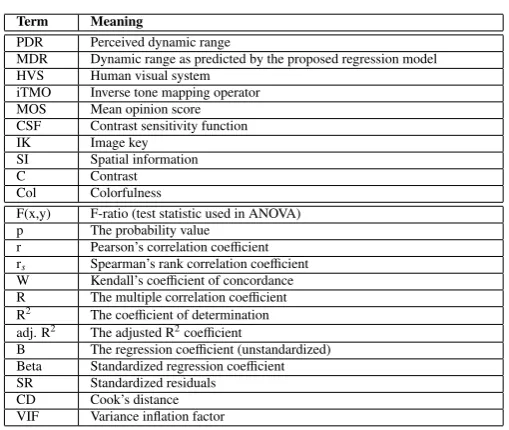
[image:3.595.36.291.415.630.2]In the rest of the paper, the abbreviations and terms pre-sented in Table 1 will be used.
Table 1: A list of abbreviations and terms used in the paper.
Term Meaning
PDR Perceived dynamic range
MDR Dynamic range as predicted by the proposed regression model HVS Human visual system
iTMO Inverse tone mapping operator MOS Mean opinion score CSF Contrast sensitivity function IK Image key
SI Spatial information C Contrast Col Colorfulness
F(x,y) F-ratio (test statistic used in ANOVA) p The probability value
r Pearson’s correlation coefficient rs Spearman’s rank correlation coefficient
W Kendall’s coefficient of concordance R The multiple correlation coefficient R2 The coefficient of determination
adj. R2 The adjusted R2coefficient
B The regression coefficient (unstandardized) Beta Standardized regression coefficient SR Standardized residuals
CD Cook’s distance VIF Variance inflation factor
2. Related Work
The study of perceived dynamic range shares some com-mon features with perceived lightness, image contrast and im-age quality. Most of these psycho-perceptual theories lack suf-ficient validation with complex stimuli, and have never been tested in HDR conditions.
1The data set is available on the project website: http://pdr.lefca.net
2.1. Perceived Lightness
Lightness is a measure of relative brightness of elements of a scene, and has been extensively studied within the field of per-ceptual psychology. One of the most popular models in light-ness perception is the intrinsic image model [13, 14, 15, 16]. This is typically based on a multi-component approach, which consists in factorizing the perceived scene as the interaction of different elements, e.g., surface reflectance, illumination and three-dimensional form or depth values. However, Gilchrist argued that these models are incomplete and proposed a new anchoring model [3], based on a combination of global and lo-cal anchoring of lightness values. On the whole, the anchoring models promote the idea that the perception of lightness is de-termined by the brightest patch of the scene. The human visual system then scales the rest to this maximum, generating an in-ternal, scene-dependent scale of light and dark. Furthermore, Li and Gilchrist [17] observed that anchoring is affected by the relativeareaof the brightest patch.
The Retinex theory [18] attempts to generate an output that is most similar to what a human observer would perceive by looking at the real scene where an image was taken. Com-pared with the anchoring theories, the Retinex theory indirectly arrives to the same conclusion through a probabilistic formu-lation. This is achieved by averaging luminance values along paths of pixels originating from each point of the picture [19], while taking into account the relative distance between patches of different brightness.
2.2. Image Contrast
While image contrast and dynamic range have similar per-ceptual connotation, they describe different aesthetic attributes. Global contrast measures [20, 21, 22] model image sharpness, which is a fine-scale image feature, as the perceptual experi-ments by Haun and Peli [23] clearly display. On the contrary, the perceived dynamic range is a measure of the magnitude of the global difference in the perceived image brightness. This is closely related to the “tone” aesthetic attribute as defined in work by Aydin et al. [8]. However, in their work this attribute is computed as a variation of the pixel-based dynamic range and does not take into account other perceptual factors. In a series of studies by Calabria and Fairchild it has been shown that per-ceived image contrast for LDR images is a function of image lightness, chroma, and sharpness [24] and the model of per-ceived image contrast and observed preference data were pro-posed [25].
2.3. Image Quality
Image quality metrics are usually based on either predicting the visibility of distortions [27, 28] or magnitude of aesthetic attributes [8]. While such metrics usually do not consider per-ceived dynamic range explicitly, there is evidence that the latter is highly related with the overall image quality. In the study by Aky¨uz et al., when two versions of the same image were com-pared, observers generally preferred the higher dynamic range one [29].
Therefore, assessing the perceived dynamic range of HDR pictures and videos can make a great contribution in design and evaluation of HDR methods, for example, inverse tone map-ping operators (iTMOs) [4, 30], where the dynamic range of LDR content is expanded for displaying on an HDR display. Most of the current approaches to enhance the perception of dy-namic range are based on heuristics. Meylan et al. [31] showed that, when expanding the dynamic range of LDR content, spec-ular highlights have to be allocated a significant range. Simi-larly, other studies tend to boost the brightest pixels of the LDR scene in order to “approximate the visceral response associated with the higher contrast and overall brightness in the original scene” [5, 4]. The results of the subjective experiment con-ducted in this paper provide a groundtruth for designing more perceptually meaningful dynamic range metrics.
Furthermore, as pointed out by Narwaria et al. [9], having a perceptually annotated HDR image dataset with MOS values is necessary for both HDR source content selection in subjective studies and for testing HDR processing algorithms. However, in that work the proposed objective measure is tailored to a dy-namic range reduction task, such as in the case of tone mapping evaluation. Moreover, no formal subjective evaluation is pro-posed to verify the perceptual relevance of that method. Predic-tive models, if successful, can serve the same role as annotated databases without requiring time-consuming data collection.
3. Motivation and Methodology
Computational metrics that predict PDR could allow for au-tomatic organization, ordering and presentation of HDR con-tent. This work’s goal is to analyze how humans perceive dy-namic range of HDR content on complex scenes, and be able to predict the PDR of a scene automatically. The research method employed involves data collection and analysis of HDR con-tent from real-world HDR images. This data is compared with objective measurements; these are subsequently used to build a PDR model. This section describes the choice of objective metrics and describes the experimental methodology.
3.1. Objective Evaluation
The objective measurements proposed here are based on the insights of a previous pilot study [10], on achromatic HDR im-ages, which inspired the work presented here; two measures (pixel-based DR and image key) are retained from the study and another three (area, contrast and colorfulness) are included based on analysis of that study’s results and previous findings on these topics [17, 24, 11]. Three objective measures were
used in the pilot study: dynamic range (DR), image key (IK) and spatial perceptual information (SI). After obtaining MOS scores, a significant correlation was found between the DR and MOS (Spearman’s rank-order correlation coefficientrs=.788;
p < .001) and IK and MOS (rs = −.671; p < .001), while
the correlation between the SI and MOS was not found to be significant (rs=.037;p=.830).
In addition, analysis of the results revealed that there might be a significant contribution to the perceived dynamic range based on the area of the brightest parts of the image. The im-ages with relatively small light sources (e.g. Zentrum, Waf-fleHouse, LasVegasStore) had the highest difference between the perceived and pixel-based DR. This is in accordance with the discussions in the literature on image contrast and anchor-ing theories where the area and distance between the contrast-ing patches have been found to be the significant image fea-tures [32, 3]. In these studies, usually two types ofwhiteare discriminated: the diffuse, below a certain threshold; and spec-ular or self-luminous, that represent values above the diffuse white threshold. A couple of studies on preferred diffuse range reported similar findings. The ITU document 6C/146-E, re-vealed that 90% of participants were satisfied with an upper limit of diffuse white being set to 2,400cd/m2[33]. In a sec-ond study, the same threshold (90% preference level) was been reported for three groups of participants with the following val-ues: 4,677cd/m2for technical, 3,090cd/m2for arts and 1,995 cd/m2for naive participants [34]. Both experiments were con-ducted on a dual modulation HDR display system [35], with the ability to reproduce luminance levels in the range from 0.004 to 20,000cd/m2. Seven images were evaluated, six of which were real-world structured stimuli, using 34 participants.
In addition, dynamic range is often confused with contrast in some contexts. Nevertheless, it was necessary to investigate perceptual relation between the two attributes, by inspecting whether a predictor of local contrast can further explain DR perception. Finally, as a number of psychophysical phenom-ena, such as the Helmhotz-Kohlrausch effect, link color appear-ance to dynamic range and contrast, colorfulness has been se-lected as an objective measure for chromatic images. The main goal was to investigate whether an attribute such as DR, gener-ally considered monochromatic, could be perceived differently when the chrominance changes even if the luminance is kept constant.
3.2. Objective Metrics
Following the results of the pilot study, DR and IK were maintained as metrics and were augmented by another three measures based on the above observations - theArea of spec-ular regions, theContrastand theColorfulness. TheAreawas motivated by the diffuse white thresholds; theContrastas the magnitude of the global lightness difference is considered as a crucial factor in perception; and theColorfulness since it is directly related to the perceived brightness of regions with con-stant luminance.
range with the following equation:
L0= L−min(L)
max(L)−min(L) ·(Dispmax−Dispmin)+Dispmin, (1)
where Dispmin = 0.03cd/m2 andDispmax = 4250cd/m2 in our setup. The DR is then calculated after excluding 1% of the darkest and brightest pixels in the image, using
DR=log10
max(L0)
min(L0), (2)
whereL0is the image with scaled values.
The image keyIK ∈ [0,1], a measure proposed by Ak¨uz and Reinhard [36], was defined as:
IK= ln(avg(L))−ln(min(L))
ln(max(L))−ln(min(L)), (3)
where the avg(L) was computed as ln(avg(L))= Σi jln(L(i,j)+ δ)/N, withδ=10−5 to avoid singularities andNwas the num-ber of pixels. Once again, min(L) and max(L) were calculated robustly, after excluding 1% of the darkest and the brightest pixels.
TheAreawas calculated as:
Area= Σi j(L(i,j)),L(i,j)>2400cd/m2, (4)
and represents the number of pixels greater than the diffuse white threshold value. The value of 2,400cd/m2 was se-lected as recommended in ITU document [33], as discussed in Section 3.1. It is in accordance with the results of the study by Daly et al. [34], where different thresholds were found for different levels of user expertise. As participants in our study ranged from naive to technical, but not necessarily in this par-ticular domain, it was reasonable to select a value towards to middle of the interval.
TheContrastmeasure is an adapted version of the work by Peli [20] and Rizzi et al. [21]. Let Lj be the image at level j
of a Gaussian pyramid, of sizeN/2j×M/2j, obtained by
dec-imating the original image with a Gaussian low-pass filter, and let N8(Lj) be the 8-neighborhood for a given pixel in Lj. In
this study, three levels were used, j ∈ [2,4], corresponding to 1.24, 2.47 and 4.95 cycle per degree (cpd), as the peaks of the contrast sensitivity function (CSF) for different light adaptation luminance lie approximately within that spatial frequency in-terval [37]. The cycles per degree were calculated based on the image dimensions, screen size and viewing distance. The contrast was computed as:
C=
P
j∈[2,4] LCj
3 , (5)
where
LCj=
P|L
j x,y−N8(Lxj,y)|
8
LWj ×LHj
, (6)
uses perceptually uniform luminance values [38]. LWj andLHj are the width and the height of the imageLat the j-th scale.
3.3. Experimental Method
The main aim of this study was to investigate the correlation between PDR and the five objective measures, for both achro-matic and chroachro-matic images, and, subsequently, to propose a model for calculating dynamic range based on these measures. Below, the design, participants, apparatus, stimuli and the ex-perimental procedure are described.
3.3.1. Design
In the study, a subjective evaluation of PDR of both achro-matic and chroachro-matic images was conducted. The participants were asked to evaluate theoverall impression of the difference between the brightest and the darkest part(s) in the images. The independent variable was the image content, while the depen-dent variable was the reported PDR of the image. The study was conducted in two separate sessions, one for achromatic and another for chromatic images; at least one day was allowed between sessions. The sessions were ordered randomly and equally.
Three possible evaluation methods are typically considered during the design of experiments of this type: paired com-parison, ranking and rating. Paired comparisons were ruled out due to their impracticality with large data sets. The effi -cient pair comparison techniques [39] can be used under certain assumptions. However, due to multidimensionality and non-deterministic DR appearance, these assumptions in our case were violated. While the ranking methods are straightforward, and quick to conduct, as with pairwise comparisons, they pro-vide no information on the magnitude of the differences. There-fore, this method has been designed in order to use the advan-tages of the three methods: it permits ranking of the stimuli, a direct comparison between the image pairs, and it uses the continuous scale for subjective scores.
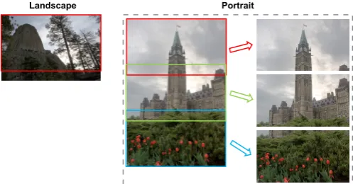
[image:5.595.308.557.492.622.2]Landscape Portrait
Figure 1: Preprocessing of the two images from the Fairchild’s data set: the landscape image (left) was first downsized from 4288×2848 to 1920×1275, and then cropped to 1920×1080 pixels; the portrait image (right) was first downsized from 2704×4015 to 1920×2851 pixels and the three HD images were cropped - top, middle and bottom.
Image
0 10 20 30 40
Dynamic range (DR)
0 1 2 3 4 5
Image
0 10 20 30 40
Image key (IK)
0.2 0.3 0.4 0.5 0.6 0.7 0.8
Image
0 10 20 30 40
Area
#104
0 5 10 15
Image
0 10 20 30 40
Contrast (C)
0 0.1 0.2 0.3 0.4
Image
0 10 20 30 40
Colorfulness (Col)
[image:6.595.72.522.89.336.2]0 10 20 30 40
Figure 2: Image features: pixel-based DR (top-left), IK (top-middle), Area (top-right), Contrast (bottom-left) and Colorfulness (bottom-right), all sorted by pixel-based DR.
selected from the pool of 137 images, and divided into three subsets of 12 pseudo-randomly selected images in a random-ized order (see section 3.3.4). The images thumbnails (422 ×
238 px) were presented across a 3×4 grid, with the correspond-ing subjective scores, initially set to zero, below each image. The red color of the score indicated that the image had not been yet evaluated. All thumbnails were tone-mapped [40] for two main reasons: the images were rather small, thus making it in-appropriate for subjective evaluation; and to discourage ratings based on the thumbnail appearance only.
The evaluation session was not time constrained. Each sub-set was evaluated independently, allowing participants to re-evaluate any image within, but not across subsets as many times as they wanted. The rating was performed on a 0-100 vertical continuous scale, divided into five equal intervals with corre-sponding labels: very low, low, medium, high and very high, included for general guidance. Upon completion, all partici-pants were interviewed, using a short structured questionnaire as described in Section 3.3.5.
3.3.2. Participants
24 participants volunteered for the study. All of them re-ported normal or corrected-to-normal visual acuity and were screened for color blindness using the Ishihara test prior to the session with chromatic images. One male participant (age 49) was found to be color blind before proceeding to the second session with chromatic images, and therefore his scores for the achromatic stimuli were discarded and not used in the analy-sis. From the remaining 23 participants 17 were male and 6 female, with the age ranging from 23 to 40 (with an average
age of 29). 12 participants were assigned to the chromatic con-dition for their first session, while the other 11 first evaluated the achromatic images during their first session.
3.3.3. Apparatus
All the experiments took place in a dark and quiet room. The stimuli were displayed at full HD (1920×1080 pixels) on an HDR SIM2 HDR47ES4MB 47” screen that allows for dis-playing>90% of Rec 709 color gamut [41]. It was utilized in the DVI Plus (DVI+) mode, that allows for directly and inde-pendently controlling backlight LEDs and LCD pixel values, based on the dual-modulation algorithm [42]. The ambient il-lumination in the room was measured between the screen and participants at 2.154lux. The luminance of the screen when turned offwas 0.03cd/m2. The distance from the screen was fixed to three heights of the display, with the eyes in the middle of the display, both horizontally and vertically.
3.3.4. Stimuli
Figure 3: The illustration of the test procedure.
Your task is to evaluate the overall impression of the difference between the darkest and the brightest part(s) of the presented images.
Figure 4: The abstraction of the attribute to be evaluated.
set are photographs of nature, a single frame from theMarket HDR video sequence proposed in MPEG by Technicolor [43] and a frame from both theCarouselandBistrovideo sequences from the Stuttgart HDR Video Database [44] were added to the test data set, see Figure 5. All 36 images were converted to the corresponding achromatic images, using BT.709 primaries to compute relative luminance [45]. In order to reproduce an im-age on the display, the luminance values should not exceed the range of the display. Values in excess of the maximum display brightness, for both the chromatic and achromatic images, were first clipped to the diplay’s peak luminance value of 4250cd/m2, and the images were then processed using the algorithm devel-oped by Zerman et al. [42] and displayed as RGB images in DVI+mode.
From the set of 36 test images, six images with the low-est and six with the highlow-est pixel-based DR were selected in two new subsets: imagesLowandimagesHigh. When generat-ing each session for the experiments, each subset of 12 images was composed of two randomly selected images from the im-agesLow subset, two fromimagesHigh and the rest from the remaining 24 images. This preserved the consistency of mea-sures among the subsets.
3.3.5. Procedure
Upon entering the experimentation room, the participants were first given the instructions to read and asked if they had any questions about the nature of the experiment and their task. This was followed by a training session, where the task was first explained using feature abstractions, inspired by the study by Aydin et al. [8], see Figure 4. They were told that in this example the magnitude of the feature increases from minimum
in the first gray block to maximum in the last, black and white block. After this, the simulation of the experimental framework was displayed with three images with high, low and average pixel-based DR range on each screen. The first three images were evaluated by the experimenter explaining that they cor-respond to the top, bottom and the middle of the rating scale respectively, and the rest of the images by the participant in or-der so stabilize their opinion. None of the six training images were part of the test data set. In both the written and verbal instructions, they were asked to evaluate the overall impression of the difference between the brightest and the darkest part(s) of the images. If the participants demonstrated a full understand-ing of the experimental task, they were asked to fill in the basic information form and the corresponding session commenced.
The images in each subset were evaluated independently; once the participant selected the next subset the results of the previous one could not be changed. However, they could eval-uate all the images in the current subset in any order and as many times as they needed. This allowed for multiple compar-isons between the images and fine adjustments of the scores. In order to evaluate an image, the participant had to click on the thumbnail. The selected HDR image was displayed full screen for evaluation. Once the participant was ready to give a rating they clicked on the presented image and a rating scale was pro-duced. The scale appeared in the far right side of the screen. After the score was given, the initial thumbnail preview of the current subset was re-displayed with the updated score for the evaluated image, see Figure 3. After the completion of the test, the experimenter had a short structured discussion about the test with all the participants. The questions used in the experiment were:
1. On a scale 1-10, how tiring was the experiment in terms of visual comfort and fatigue?
• Have you been bothered by some particular im-ages?
2. On a scale 1-10, how difficult did you find it to evaluate the images?
• What did you find difficult? Why? Which (type of) images?
3. With how many ratings are you confident (you think your score is correct)?
[image:7.595.85.242.226.331.2]507 AirBellowsGap BandonSunset(1) BigfootPass
Bistro BloomingGorse(1) Carousel DelicateFlowers
DevilsTower ElCapitan b Flamingo GoldenGate(1)
HancockKitchenInside HancockKitchenOutside HDRMark JesseBrownsCabin
LabBooth LabTypewriter LasVegasStore Market3
NorthBubble OCanadaNoLights b OCanadaNoLights m OtterPoint
PaulBunyan PeckLake SequoiaRemains t TupperLake(1)
URChapel(1) t URChapel(2) b URChapel(2) m WaffleHouse
[image:8.595.20.566.82.738.2]WillyDesk WillySentinel b WillySentinel m Zentrum
Table 2: Pearson’srand Spearman’srscorrelation coefficients between MOS values for both achromatic and chromatic images and
five objective measures: DR, IK, Area, C and Col. * denotes significance at p<.01.
MOS Achromatic Chromatic
Measure DR IK Area’ C DR IK Area’ C Col
r .87* -.60* .87* -.19 .84* -.61* .87* -.22 -.47* rs .87* -.55* .89* -.24 .84* -.57* .90* -.27 -.43*
• If so, what? How? Why?
5. Is there anything else you would like to comment on? 6. Was it easier to evaluate grayscale or color images?2
4. Results
Results were analyzed with a series of statistical tests to form a better understanding of the captured data. This section presents results across the participants testing for group, image and chromatic conditions and correlations comparing MOSs with the objective measurements.
4.1. Overall Results Across Participants
The effect of the independent variables on the PDR scores provided by the participant was analyzed in a 2 (session)
× 2 (color) × 36 (scenes) factorial design. session is a between-participants variable reflecting the order of chromatic-achromatic presentation whereby 12 participants were first pre-sented with the chromatic condition and the other 11 with the achromatic condition on their first session. coloris a within-participants variable that corresponds to the chromatic and achromatic results andscenesis also a within-participants vari-able corresponding to the 36 images presented to the partici-pants.
Results were analyzed using a mixed-model factorial ANOVA. The main effect ofsession was not significant F(1, 21)=2.06 , p=.17. This indicates that the session ordering did not have a significant effect on the results.
The main effect ofcolorwas also insignificant, F(1, 21)= .40 , p=.40. Again this indicates that there was no significant difference between the scores for the chromatic and achromatic set. Further analysis of the chromatic and achromatic results is given below.
The main effect ofsceneswas significant F(35, 735)=98.73 , p<.01 as expected. Analysis of the differences and correla-tions with objective measurements will be given below.
In order to analyze the agreement across participant scores, Kendall’s coefficient of concordanceW was employed. W re-ports a value of 1 for absolute agreement across all judges and 0 for complete disagreement. For the achromatic condition, Kendall’s coefficient of concordance was significant (W =.81, p<.01) and similarly for the chromatic condition (W =.76, p
<.01). These results indicate a very strong agreement across participants’ allocated scores.
4.2. Correlations of MOS
In order to analyze the correlations among the PDR values provided by the participants per scene, results were collapsed into a mean opinion score (MOS) per scene. The MOSs are correlated with the four (five for chromatic) objective measures presented in Section 3.2. The scatter plots for each of the five objective measures are provided in Figure 6 and Figure 7.
Since the calculated measures were on different scales, they were scaled using the equation:
x0i= xi− 1
n Pn
i=1xi
max(X)−min(X) (7)
so that they are all represented with the same order of magni-tude. The results of the correlation between the MOS values and objective measures can be seen in Table 2.
Initially, when comparing the Pearson’s (r) and Spearman’s (rs) correlation coefficients, the only substantial difference was
found for the Area measure (r = .64 andrs = .87 for
achro-matic, and r = .64 andrs = .88 for chromatic stimuli). By
observing the correlation scatter plots (Figures 6 and 7), an evi-dent trend of the root function was noticeable for this measure. A number of root functions were tested in order to linearize the data and the best was found to be:
Area0= 4
√
Area. (8)
With the fitted data (Area0) the Pearson’s correlation coefficient was almost identical to the Spearman’s (see Table 2), which eventually resulted in a more robust predictor model, see Sec-tion 5.
The correlations between the chromatic MOS and achro-matic MOS werer=.99 andrs=.98, both significant at p<
.01, indicating the chromatic and achromatic scores were very highly correlated.
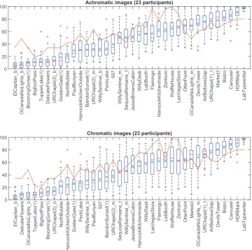
In Figure 8, the extended box plot depicts the distribution of the perceived DR scores, with the corresponding mean and median values, confidence intervals and outliers. In addition, the pixel-based DR is also presented to visually display the cor-relation between the subjective and objective scores.
4.3. Post-experimental Inquiry
The comments obtained upon completion of each session of the study were fairly consistent across all the questions. The av-erage score of the answer to the first question was 3.93, which means that there were instances which were slightly annoying
Dynamic range (DR)
0 1 2 3 4 5
MOS
0 20 40 60 80 100
Image key (IK)
0.2 0.4 0.6 0.8
MOS
0 20 40 60 80 100
Area #104
0 5 10 15
MOS
0 20 40 60 80 100
Contrast (C)
0 0.1 0.2 0.3 0.4
MOS
[image:10.595.62.527.108.359.2]0 20 40 60 80 100
Figure 6: Achromatic MOS across the four objective measures (top-left to bottom-right): pixel-based DR, IK, Area and Contrast.
Dynamic range (DR)
0 1 2 3 4 5
MOS
0 20 40 60 80 100
Image key (IK)
0.2 0.4 0.6 0.8
MOS
0 20 40 60 80 100
Area #104
0 5 10 15
MOS
0 20 40 60 80 100
Contrast (C)
0 0.1 0.2 0.3 0.4
MOS
0 20 40 60 80 100
Colorfulness (Col)
0 10 20 30 40
MOS
0 20 40 60 80 100
[image:10.595.70.524.443.695.2]to observe. Around 60% of participants reported that the bright-est images with the visible sun or light sources were uncomfort-able to look at.
The average score to the second question was 4.17. Sev-eral participants reported that the images with “very small but very bright portions of the image” were more difficult to eval-uate and that the area of the brightest parts (i.e. light sources, sun) could have an affect on the perception of DR. A number of participants mentioned that they think that the PDR varies de-pending on the proximity of the brightest and the darkest parts in the image. For example, if there is the sun in one corner of the image and a part of the scene in shadow in the other corner (e.g. OtterPoint) versus if there is the sun behind the tree (e.g. DevilsTower).
It was reported that the user confidence for the given scores (question 3; i.e. images that were relatively easy to evaluate and to which they think they gave an objective score) was 70.74%. The images constituting the remaining 29.26% correspond to the images with a medium DR, which was in accordance with the increased confidence interval for these images, see Figure
8.
Generally, all the participants liked the experimental design and there were no major complaints regarding the framework (question 4). One participant suggested that it might be better to have more than 12 images in a subset. Initially, there were two subsets, each consisting of 20 images. However, the pilot study revealed that it might be too difficult to perform comparisons among that many images. Furthermore, ten images are used in the SAMVIQ methodology, upon which this framework had been developed.
In the general comments section (question 5), the partici-pants reported that the possibility of re-evaluating images was very helpful and liked the fact that they could evaluate images in any order without time constraints. They also reported that the overall image brightness might be affecting the PDR.
The responses to the last question revealed that it was slightly easier to evaluate achromatic images (60.87% of par-ticipants) as opposed to chromatic (26.09%). 13.04% of partic-ipants reported that it was the same in terms of difficulty. Most of the participants from the first group (i.e. the 60.87% who
ElCapitan_b
OCanadaNoLights_b BloomingGorse(1)
BigfootPass
TupperLake(1) DelicateFlowers URChapel(2)_b GoldenGate(1) NorthBubble PaulBunyan
HancockKitchenOutside
BandonSunset(1) URChapel(2)_m WillySentinel_b
PeckLake
507
WillySentinel_m
SequoiaRemains_t JesseBrownsCabin WillyDesk LabBooth Flamingo
HancockKitchenInside
Zentrum
WaffleHouse
LasVegasStore
OtterPoint
OCanadaNoLights_m
DevilsTower
AirBellowsGap URChapel(1)_t
Market3 Bistro Carousel HDRMark
LabTypewriter
0 20 40 60 80
100 Achromatic images (23 participants)
ElCapitan_b
DelicateFlowers
OCanadaNoLights_b
TupperLake(1) BigfootPass BloomingGorse(1) URChapel(2)_b
NorthBubble
HancockKitchenOutside
GoldenGate(1)
PeckLake
WillySentinel_b
PaulBunyan
507
BandonSunset(1) URChapel(2)_m SequoiaRemains_t WillySentinel_m JesseBrownsCabin
HancockKitchenInside
WillyDesk
LasVegasStore
Flamingo LabBooth
WaffleHouse
Zentrum OtterPoint Market3
OCanadaNoLights_m
URChapel(1)_t AirBellowsGap DevilsTower
Bistro
Carousel HDRMark
LabTypewriter
0 20 40 60 80
[image:11.595.120.481.344.702.2]100 Chromatic images (23 participants)
Table 3: The summary of the model withR,R2, adjustedR2 and F change significance values for both achromatic and chromatic images, presented across the hierarchies.
Achromatic Chromatic
Model R R2 adj.
R2
sig. F
change R R
2 adj. R2
sig. F change
DR .866 .750 .743 .000 .839 .704 .695 .000 DR, Area’ .945 .893 .887 .000 .932 .868 .860 .000
found achromatic easier) reported that this could be due to the extra chromatic information which compounded the complexity of the choice.
These comments were a valuable input to the study and were considered when choosing the predictors in the regression model (see Section 5).
5. PDR Predictor Model
This section looks into producing a model that can predict PDR based on the results of the experiment. To achieve this, multivariate linear regression is employed and analyzed.
5.1. Creating the Model
The results from the pilot study [10] and the previous sec-tion indicate that the pixel-based DR is a generally good predic-tor of the PDR, but there are cases where it fails (see Section 6), and that it could be potentially improved if other measures are considered. The results were also used as an indication of the measures that could be used as variables for predicting the out-come in the multiple regression analysis. In particular, a model is fit to the data and used to predict values of the outcome from several predictors.
[image:12.595.309.563.291.405.2]Miles and Shelvin [46] suggest that when expecting a large effect size, a sample size of around 40 is sufficient for two to four predictors. This is close to our initial sample of 36 images. Prior to employing the regression, the data for the Area mea-sure was linearized using the Equation 8, and all the meamea-sures were feature-scaled using Equation 7. The hierarchical method was utilized in order to see the behavior of the model with new predictors. Since pixel-based DR was known to be a good pre-dictor of the perceived DR, it was selected for the first block in the hierarchy. The forced entry method was selected for DR. All other predictors (IK, Area’, C and Col) were added to the second block. For this block, the forward method was used. This method calculates the contribution of each predictor by looking at the semi-partial correlation with the outcome. The model summary with the correspondingR,R2, adjustedR2and the significance of the F change values are presented in Table 3. TheRvalues show the multiple correlation coefficients be-tween the predictors and the outcome. In the first case where there is only one predictor (DR), this is a simple correlation be-tween MOS and this measure. In case of achromatic images, theRvalue increases from.866 with DR only, to.945 with DR and Area’ measures. SimilarRvalues can be observed for the chromatic images (R =.839 for DR andR=.932 for DR and Area’ measures).
Table 4: EstimatedBetaInvalue, t-statistics and its significance for each predictor. For both achromatic and chromatic models the Area’ predictor has the highest (significant)tvalue, and was therefore included in the model. In the following iteration none of the remaining variables (IK, C and Col for the chromatic model) had significanttvalue, and thus were not included into the model.
Achromatic Chromatic
Model BetaIn t S ig. BetaIn t S ig.
IK -.137 -1.303 .202 -.181 -1.610 .117 Area’ .516 6.657 .000 .553 6.418 .000 C -.113 -1.325 .194 -.150 -1.640 .110
Col -.219 -2.362 .024
IK .069 .889 .381 .031 .361 .720
C -.049 -.838 .408 -.082 -1.291 .206
[image:12.595.307.558.449.558.2]Col -.116 -1.725 .094
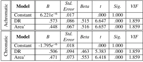
Table 5: Model parameters for the achromatic and chromatic images.
Achromatic
Model B Std.
Error Beta t Sig. VIF
Constant 6.221e−6 .017 .000 1.000
DR .573 .086 .515 6.647 .000 1.859
Area’ .448 .067 .516 6.657 .000 1.859
Chromatic
Model B Std.
Error Beta t Sig. VIF
Constant -1.795e−6 .018 .000 1.000
DR .506 .094 .463 5.383 .000 1.859
Area’ .471 .073 .553 6.418 .000 1.859
In the stepwise regression, at each iteration, the BetaIn value is estimated for each predictor that has not been included into the model, as if it were entered into equation at this stage. The standardized b-value,BetaIn, indicates the number of stan-dard deviations that the outcome will change as a result of one standard deviation change in the predictor. Based on this value, the t-statistics for these values are computed and based on its significance the next predictor is entered, until there are no pre-dictors with significant value less than .05, see Table 4.
5.2. The Model Parameters
Therefore, the regression model for the achromatic images is defined as:
MDR≈0.573DR+0.4484
√
Area (9)
while for the chromatic images it is:
MDR≈0.506DR+0.4714
√
Area (10)
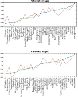
In Figure 9 the observed scores (MOS), pixel-based DR and MDR values are displayed for each scene. A significantly higher correlation between the MOS and MDR than between the MOS and pixel-based DR is evident. The cases with the highest discrepancy between the latter will be further discussed in Section 6.
In order to verify whether the model fits the data or if it is skewed by a few extreme cases (outliers), the standardized residuals (SR), obtained by dividing the residual by an esti-mate of their standard deviation, were examined. In addition,
Cook’s distance (CD) was calculated in order to check for the influential cases [47]. This test analyzes whether the regres-sion model is stable across the sample, by calculating the over-all influence of a particular case on the model. Based on the findings by Cook and Weisberg [48], values greater than 1 may be cause for concern. Computing the residual statistics on a case-wise basis, the results revealed that there were no cases with the absolute value of the SR greater than 3.29. For three achromatic images:HancockKitchenInside, OCanadaNo-Lights bottomandSequoiaRemains topthis value was−2.25,
−2.441 and 2.238 respectively. In the case of chromatic images there was onlyHancockKitchenInsideimage for which the SR value was−2.748. Cook’s distance (CD) for the three achro-matic images was .170, .167 and .087 respectively, while for theHancockKitchenInsidechromatic image this value was.253 respectively. Therefore, based on these results, the sample rep-resents an accurate model.
Multicollinearity between predictors makes it difficult to as-sess the individual contribution of a predictor. If the two
pre-ElCapitan_b
OCanadaNoLights_b
BloomingGorse(1)
BigfootPass
TupperLake(1)
DelicateFlowers URChapel(2)_b GoldenGate(1) NorthBubble PaulBunyan
HancockKitchenOutside
BandonSunset(1) URChapel(2)_m WillySentinel_b
PeckLake
507
WillySentinel_m
SequoiaRemains_t JesseBrownsCabin WillyDesk LabBooth Flamingo
HancockKitchenInside
Zentrum
WaffleHouse
LasVegasStore
OtterPoint
OCanadaNoLights_m
DevilsTower
AirBellowsGap URChapel(1)_t
Market3
Bistro
Carousel HDRMark
LabTypewriter
-60 -40 -20 0 20 40
60 Achromatic images
ElCapitan_b
DelicateFlowers
OCanadaNoLights_b
TupperLake(1)
BigfootPass
BloomingGorse(1)
URChapel(2)_b
NorthBubble
HancockKitchenOutside
GoldenGate(1)
PeckLake
WillySentinel_b
PaulBunyan
507
BandonSunset(1) URChapel(2)_m
SequoiaRemains_t
WillySentinel_m
JesseBrownsCabin
HancockKitchenInside
WillyDesk
LasVegasStore
Flamingo LabBooth
WaffleHouse
Zentrum
OtterPoint Market3
OCanadaNoLights_m
URChapel(1)_t AirBellowsGap
DevilsTower
Bistro
Carousel HDRMark
LabTypewriter
-60 -40 -20 0 20 40
[image:13.595.152.452.333.704.2]60 Chromatic images
dictors are highly correlated, there is a high possibility that each accounts for similar variance in the outcome. Multicollinearity was tested by using the variance inflation factor (VIF), see Ta-ble 5. As argued by Myers, a value greater than 10 indicates a potential problem [49]. In addition, values less than 0.2 indi-cate a potential multicollinearity and should be further investi-gated [50]. As VIF values for both achromatic and chromatic models were 1.859, there is no indication of multicollinearity between the predictors in the models.
5.3. Calculating Model Generalizability
TheR2values show how much of the variability in the MOS is accounted for by the predictors. For the achromatic images using only DR as a predictor R2 = .75, while for the same model with chromatic imagesR2=.704, which means that DR accounts for 75% and 70.4% of total variation of the MOS re-spectively. Adding Area’ as the second predictor, this percent-age rises to 89.3% for achromatic, and 86.8% for chromatic.
Finally, for assessing how well the sample represents the entire population, that is how accurately the model can pre-dict the outcome in a different sample, a cross-validation of the model was performed. If the prediction on another sample is similarly correct, then the model can be generalized. Cross-validation was calculated by adjusting theR2values by estimat-ing how theR2 values were derived from the population from which the sample was taken. The adjustedR2 values give an indication of how well the model generalizes. The closer the values to the R2 ones are, the better the prediction from the sample is. For example, the difference between theR2and the adjustedR2 values for the achromatic model with two predic-tors is 0.893−0.887 = 0.006, which means that if the model was derived from the population, instead of from the sample, it would account for 0.6% less variance in the MOS. The values presented in Table 3 indicate a very good cross-validity of the model.
Calculating the change statistics, the significance of the change inR2by adding new predictors can be calculated. This is usually done by calculating the F-ratio by using the following equation:
F=(N−k−1)R 2
k(1−R2) (11)
whereNis the number of cases, andkis the number of predic-tors in the model.
In Table 3, a significance of the F change is provided. In both the achromatic and chromatic image models, there was a significant change inR2 value for addition of the Area’ (p <
.001).
6. Analysis of High Discrepancy Scenes
As was shown in Section 4, a straightforward metric such as pixel-based DR can be a good predictor of dynamic range for many of the images. However, there are some particular cases where it fails to truthfully predict the PDR. In this sec-tion the scenes with highest discrepancies between pixel-based
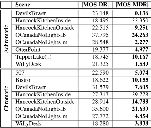
[image:14.595.306.556.245.456.2]DR and MOS values are investigated, for both the achromatic and chromatic images. Two subsets of eight scenes with the highest discrepancies were selected, see Figure 10. The values obtained by taking the absolute value of the subtracted feature-scaled scores are presented in Table 6.
Table 6: Eight achromatic (top) and eight chromatic (bottom) scenes with the highest difference between the MOS and pixel-based DR, along with the differences between the MOS scores and predicted perceived dynamic range by the proposed model (MDR). The scores are calculated as the absolute difference be-tween the feature-scaled values obtained using Equation 7), and multiplied by 100 for better readability.
Scene |MOS-DR| |MOS-MDR|
Achromatic
DevilsTower 23.148 0.136
HancockKitchenInside 18.495 22.350 HancockKitchenOutside 22.515 9.251 OCanadaNoLights b 37.795 24.263 OCanadaNoLights m 28.548 2.277
OtterPoint 19.377 4.977
TupperLake(1) 18.745 10.167
WillyDesk 21.325 1.539
Chromatic
507 22.590 5.074
Bistro 18.622 10.155
DevilsTower 31.579 7.605
HancockKitchenInside 27.317 29.778 HancockKitchenOutside 28.914 14.788 OCanadaNoLights b 35.600 21.639 OCanadaNoLights m 27.772 4.854
WillyDesk 18.280 3.838
These results demonstrate that in 14 out of the 16 cases the model predicts the PDR better than the pixel-based DR mea-sure. Table 7 shows the correlations between the MOS scores and both pixel-based DR and MDR, performed on these sub-sets. For both achromatic and chromatic scenes, the correlation between the MOS and DR is not significant (p>0.05). Nev-ertheless, the correlation between the MOS and predicted per-ceived dynamic range (MDR) is significant in all cases. These chosen cases demonstrate why the predictive method can be considered superior to the DR method when predicting PDR.
Table 7: The Pearson’srand Spearman’srscorrelation coeffi
-cients between MOS values and both pixel-based DR and MDR for achromatic and chromatic scenes. *Correlation significant at p<.01; **Correlation significant at p<.05.
MOS Achromatic Chromatic
Measure DR MDR DR MDR
r .584 .912* .354 .881*
[image:14.595.335.527.657.710.2]DevilsTower HancockKitchenIn HancockKitchenOut OCanadaNoLights b
OCanadaNoLights m OtterPoint TupperLake(1) WillyDesk
507 Bistro DevilsTower HancockKitchenIn
[image:15.595.109.488.91.390.2]HancockKitchenOut OCanadaNoLights b OCanadaNoLights m WillyDesk
Figure 10: Achromatic (top) and chromatic (bottom) high discrepancy images used in the analysis.
7. Conclusions and Future Work
While traditional dynamic range measures can be an ac-ceptable predictor of PDR, they can also be inaccurate in some cases. In order to develop a generic model that can truthfully predict PDR, sensory and cognitive processes involved in ex-traction of this attribute from complex stimuli need to be taken into account. Previous research has shown that the area of the brightest patches and the image topology affect the perception of lightness and contrast [17, 19, 26], and therefore should be considered in constructing such a PDR model. Furthermore, image contrast and colorfulness are important factors in visual perception and, based on previous findings [8, 11, 24, 25], could be involved in the process related to the extraction of observed image attributes.
In this study a new experiment for subjective evaluation of perceived dynamic range in HDR images has been designed and conducted. The results were used to generate a subjectively annotated data set of 36 HDR images, with both MOS scores for achromatic and chromatic data. This data set can be used in future HDR content studies on algorithm or metric validation and aesthetic attribute analysis and modeling. This is, to the best of the authors’ knowledge, the first study on perceived DR using complex stimuli and HDR conditions.
The results of the Kendall’s coefficient of concordance show that there was a high agreement between participants’ scores in both sessions. Using the mixed model factorial ANOVA the
ef-fect of scenes was found as significant, while neither the session order nor chromaticity of the data were found to produce signif-icant differences in the results. In addition, the correlation be-tween the chromatic and achromatic MOSs was computed, and the results demonstrated very high correlations. Furthermore, the correlations between the PDR and five objective measures were computed. All correlations, except for the contrast (C), were found as significant for both achromatic and chromatic images, with very small discrepancies between the two condi-tions.
Models that can predict PDR of both achromatic and chro-matic images were generated using multivariate linear regres-sion. The regression model revealed that only pixel-based DR and linearized Area measures had significant contribution to the predictor model. Cross-validation of the model showed that the model could accurately predict the outcome in a different sam-ple, i.e. the model can be generalized.
Finally, eight scenes with the highest discrepancies between the MOS and pixel-based DR values were selected from both achromatic and chromatic sets. The statistics showed that the PDR prediction was significantly improved when the Area pre-dictor contributed to the model.
the perception of such visual attributes. Therefore, in the fu-ture, we would like to further investigate this topic by looking at these and other perceptual factors that could be involved in this process at a lower level. Furthermore, the existing objective metrics have to be redesigned and, possibly, novel ones devel-oped targeted directly at HDR content. While this is beyond the scope of this paper, it was evident that a gap exists in this area. Another direction at which we would like to expand this work is the analysis of aesthetic attributes. Finally, we are inter-ested in extending this work to video content and investigating the temporal aspects. In the case of video, the perceptual phe-nomena behind the perception of dynamic range can be more complex. While, for a static image, the luminance range repro-ducible by an HDR display matches the steady-state dynamic range of the HVS, temporal variations of this range, e.g., due to a change from a bright to a dark scene, can span a much broader interval of luminance than the HVS could process at a given adaptation level, causing maladaptation phenomena and visual discomfort [37]. It is known that light/dark adaptation is not instantaneous, which results in higher masking for larger temporal variations of the luminance range. This entails a loss of contrast sensitivity in the maladaptation phase, but could en-hance the overall perception of bright-dark differences on short time segments. Therefore, initial studies will be conducted with a similar methodology, using short clips, and the scores will be correlated with dynamic range models similar to those dis-cussed in this work.
8. Acknowledgments
The authors would like to thank Emin Zerman for the help with the DVI+content generation and with development of the test framework. We would like to thank all the participants that volunteered in the subjective study. This work was supported by Region Ile de France, in the framework of the FUI 4EVER2 project. Debattista is partially supported by a Royal Society Industrial Fellowship.
References
[1] F. Banterle, A. Artusi, K. Debattista, A. Chalmers, Advanced high dy-namic range imaging: theory and practice, CRC Press, 2011.
[2] F. Dufaux, P. Le Callet, R. Mantiuk, M. Mrak, High Dynamic Range Video. From Acquisition, to Display and Applications, Academic Press, 2016.
[3] A. Gilchrist, C. Kossyfidis, F. Bonato, T. Agostini, J. Cataliotti, X. Li, B. Spehar, V. Annan, E. Economou, An anchoring theory of lightness perception., Psychological review 106 (4) (1999) 795.
[4] F. Banterle, P. Ledda, K. Debattista, A. Chalmers, Inverse tone mapping, in: Proc. of the 4th International Conference on Computer Graphics and Interactive Techniques in Australasia and Southeast Asia, GRAPHITE ’06, ACM, New York, NY, USA, 2006, pp. 349–356. doi:10.1145/ 1174429.1174489.
URLhttp://doi.acm.org/10.1145/1174429.1174489
[5] A. G. Rempel, M. Trentacoste, H. Seetzen, H. D. Young, W. Heidrich, L. Whitehead, G. Ward, LDR2HDR: On-the-fly reverse tone mapping of legacy video and photographs, in: ACM SIGGRAPH 2007 Papers, SIGGRAPH ’07, ACM, New York, NY, USA, 2007. doi:10.1145/ 1275808.1276426.
URLhttp://doi.acm.org/10.1145/1275808.1276426
[6] F. De Simone, G. Valenzise, P. Lauga, F. Dufaux, F. Banterle, Dynamic range expansion of video sequences: A subjective quality assessment study, in: IEEE Global Conference on Signal and Information Process-ing, IEEE, 2014, pp. 1063–1067.
[7] C. Mantel, J. Korhonen, S. Forchhammer, J. Pedersen, S. Bech, Subjec-tive quality of videos displayed with local backlight dimming at different peak white and ambient light levels, in: 7th Int. Work. on Quality of Mul-timedia Experience, IEEE, 2015, pp. 1–6.
[8] T. O. Aydin, A. Smolic, M. Gross, Automated aesthetic analysis of pho-tographic images, Visualization and Computer Graphics, IEEE Transac-tions on 21 (1) (2015) 31–42.
[9] M. Narwaria, C. Mantel, M. Perreira de Silva, P. Le Callet, An objective method for High Dynamic Range source content selection, in: 6th Int. Work. on Quality of Multimedia Experience, 2014, pp. 13–18.
[10] V. Hulusic, G. Valenzise, E. Provenzi, K. Debattista, F. Dufaux, Perceived dynamic range of HDR images, in: Proceedings 8th International Work-shop on Quality of Multimedia Experience (QoMEX2016), IEEE, 2016. [11] M. D. Fairchild, Color appearance models, John Wiley & Sons, 2013. [12] J.-L. Blin, SAMVIQ - Subjective assessment methodology for video
qual-ity, Rapport technique BPN 56 (2003) 24.
[13] S. S. BERGSTROM, Common and relative components of reflected light as information about the illumination, colour, and three-dimensional form of objects, Scandinavian journal of psychology 18 (1) (1977) 180–186. [14] H. Barrow, J. Tenenbaum, Recovering intrinsic scene characteristics,
Comput. Vis. Syst., A Hanson & E. Riseman (Eds.) (1978) 3–26. [15] A. L. Gilchrist, The perception of surface blacks and whites, WH
Free-man, 1979.
[16] E. H. Adelson, A. P. Pentland, The perception of shading and reflectance, Perception as Bayesian inference (1996) 409–423.
[17] X. Li, A. L. Gilchrist, Relative area and relative luminance combine to an-chor surface lightness values, Perception & Psychophysics 61 (5) (1999) 771–785.
[18] E. H. Land, J. J. McCann, Lightness and retinex theory, JOSA 61 (1) (1971) 1–11.
[19] E. Provenzi, L. De Carli, A. Rizzi, D. Marini, Mathematical definition and analysis of the retinex algorithm, Journal of the Optical Society of America A 22 (12) (2005) 2613–2621.
[20] E. Peli, Contrast in complex images, JOSA A 7 (10) (1990) 2032–2040. [21] A. Rizzi, T. Algeri, G. Medeghini, D. Marini, A proposal for contrast
measure in digital images, in: Conference on Colour in Graphics, Imag-ing, and Vision, Vol. 2004, Society for Imaging Science and Technology, 2004, pp. 187–192.
[22] K. Matkovic, L. Neumann, A. Neumann, T. Psik, W. Purgathofer, Global contrast factor-a new approach to image contrast., Computational Aes-thetics 2005 (2005) 159–168.
[23] A. M. Haun, E. Peli, 24.1: Measuring the perceived contrast of natural images, in: SID Symposium Digest of Technical Papers, Vol. 42, Wiley Online Library, 2011, pp. 302–304.
[24] A. J. Calabria, M. D. Fairchild, Perceived image contrast and observer preference i. the effects of lightness, chroma, and sharpness manipulations on contrast perception, Journal of imaging Science and Technology 47 (6) (2003) 479–493.
[25] A. J. Calabria, M. D. Fairchild, Perceived image contrast and observer preference ii. empirical modeling of perceived image contrast and ob-server preference data, Journal of Imaging Science and Technology 47 (6) (2003) 494–508.
[26] P. Vangorp, K. Myszkowski, E. W. Graf, R. K. Mantiuk, A model of local adaptation, ACM Transactions on Graphics (TOG) 34 (6) (2015) 166. [27] S. Winkler, Chapter 5: Perceptual video quality metrics–a review, Digital
Video Image Quality and Perceptual Coding (2006) 155–179.
[28] J. Kopf, W. Kienzle, S. Drucker, S. B. Kang, Quality prediction for image completion, ACM Trans. Graph. 31 (6) (2012) 131:1–131:8. doi:10. 1145/2366145.2366150.
URLhttp://doi.acm.org/10.1145/2366145.2366150
[29] A. O. Aky¨uz, R. Fleming, B. E. Riecke, E. Reinhard, H. H. B¨ulthoff, Do HDR displays support ldr content?: a psychophysical evaluation, in: ACM Transactions on Graphics (TOG), Vol. 26, ACM, 2007, p. 38. [30] F. Banterle, P. Ledda, K. Debattista, M. Bloj, A. Artusi, A. Chalmers, A
psychophysical evaluation of inverse tone mapping techniques, Computer Graphics Forum 28 (1) (2009) 13–25.
[31] L. Meylan, S. Daly, S. Susstrunk, The reproduction of specular highlights on high dynamic range displays, in: Proc. of the 14th Color Imagining Conference, 2006.
[32] M. D. Fairchild, The HDR photographic survey, in: Color and Imag-ing Conference, Vol. 2007, Society for ImagImag-ing Science and Technology, 2007, pp. 233–238.
[33] ITU-R, Proposed preliminary draft new Report - Image dynamic range in television systems, ITU-R WP6C Contribution 146 (April 2013). [34] S. Daly, T. Kunkel, X. Sun, S. Farrell, P. Crum, 41.1: Distinguished paper:
Viewer preferences for shadow, diffuse, specular, and emissive luminance limits of high dynamic range displays, in: SID Symposium Digest of Technical Papers, Vol. 44, Wiley Online Library, 2013, pp. 563–566. [35] H. Seetzen, L. A. Whitehead, G. Ward, 54.2: A high dynamic range
dis-play using low and high resolution modulators, in: SID Symposium Di-gest of Technical Papers, Vol. 34, Wiley Online Library, 2003, pp. 1450– 1453.
[36] A. O. Aky¨uz, E. Reinhard, Color appearance in high-dynamic-range imaging, Journal of Electronic Imaging 15 (3) (2006) 033001–033001. [37] S. Kunkel, S. Daly, M. J. Froehlich, Perceptual design for high dynamic
range systems, in: F. Dufaux, P. Le Callet, R. Mantiuk, M. Mrak (Eds.), High Dynamic Range Video. From Acquisition, to Display and Applica-tions, Academic Press, 2016, Ch. 15, pp. 391–430.
[38] T. O. Aydın, R. Mantiuk, H. Seidel, Extending quality metrics to full dynamic range images, in: Proc. of SPIE Electronic Imaging: Human Vision and Electronic Imaging XIII, San Jose, USA, 2008, pp. 6806–10. [39] D. A. Silverstein, J. E. Farrell, Efficient method for paired comparison,
Journal of Electronic Imaging 10 (2) (2001) 394–398.
[40] R. Mantiuk, S. Daly, L. Kerofsky, Display adaptive tone mapping, ACM Transactions on Graphics (TOG) 27 (3) (2008) 68.
[41] SIM2, http://www.sim2.com/hdr/(Jun. 2014). URLhttp://www.sim2.com/HDR/
[42] E. Zerman, G. Valenzise, F. De Simone, F. Banterle, F. Dufaux, Effects of display rendering on HDR image quality assessment, in: SPIE Optical Engineering+Applications, International Society for Optics and Photon-ics, 2015, pp. 95990R–95990R.
[43] S. Lasserre, F. LeL´eannec, E. Francois, Description of HDR sequences proposed by technicolor, ISO/IEC JTC1/SC29/WG11 JCTVC-P0228, IEEE, San Jose, USA.
[44] J. Froehlich, S. Grandinetti, B. Eberhardt, S. Walter, A. Schilling, H. Brendel, Creating cinematic wide gamut HDR-video for the evalua-tion of tone mapping operators and HDR-displays (2014).arXiv:http: //spiedigitallibrary.org.
URLhttp://spiedigitallibrary.org
[45] ITU-T, Parameter values for the HDTV standards for the studio and for international programme exchange., Recommendation BT.709 (1993). [46] J. Miles, M. Shevlin, Applying regression and correlation: A guide for
students and researchers, Sage, 2001.
[47] R. D. Cook, Detection of influential observation in linear regression, Technometrics 19 (1) (1977) 15–18.
[48] R. D. Cook, S. Weisberg, Residuals and influence in regression. [49] R. Myers, Classical and modern regression with applications. boston:
Pws and kent publishing company (1990).