Coupled bulk surface free boundary problems arising from a mathematical model of receptor ligand dynamics

Original citation:

Elliott, Charles M., Ranner, Thomas and Venkataraman, Chandrasekhar. (2017) Coupled

bulk-surface free boundary problems arising from a mathematical model of receptor-ligand

dynamics. SIAM Journal on Mathematical Analysis, 49 (1). pp. 360-397.

Permanent WRAP URL:

http://wrap.warwick.ac.uk/83693

Copyright and reuse:

The Warwick Research Archive Portal (WRAP) makes this work of researchers of the

University of Warwick available open access under the following conditions. Copyright ©

and all moral rights to the version of the paper presented here belong to the individual

author(s) and/or other copyright owners. To the extent reasonable and practicable the

material made available in WRAP has been checked for eligibility before being made

available.

Copies of full items can be used for personal research or study, educational, or not-for-profit

purposes without prior permission or charge. Provided that the authors, title and full

bibliographic details are credited, a hyperlink and/or URL is given for the original metadata

page and the content is not changed in any way.

Publisher’s statement:

First Published in SIAM Journal on Mathematical Analysis in 49 (1), 2017 published by the

Society for Industrial and Applied Mathematics (SIAM). Copyright © by SIAM. Unauthorized

reproduction of this article is prohibited.

Published version:

http://dx.doi.org/10.1137/15M1050811

A note on versions:

The version presented in WRAP is the published version or, version of record, and may be

cited as it appears here.

COUPLED BULK-SURFACE FREE BOUNDARY PROBLEMS ARISING FROM A MATHEMATICAL MODEL OF

RECEPTOR-LIGAND DYNAMICS∗

CHARLES M. ELLIOTT†, THOMAS RANNER‡, AND CHANDRASEKHAR VENKATARAMAN§

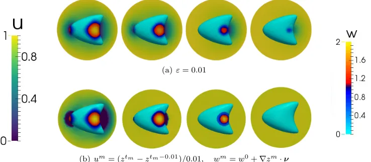
Abstract. We consider a coupled bulk-surface system of partial differential equations with nonlinear coupling modeling receptor-ligand dynamics. The model arises as a simplification of a mathematical model for the reaction between cell surface resident receptors and ligands present in the extracellular medium. We prove the existence and uniqueness of solutions. We also consider a number of biologically relevant asymptotic limits of the model. We prove convergence to limiting problems which take the form of free boundary problems posed on the cell surface. We also report on numerical simulations illustrating convergence to one of the limiting problems as well as the spatiotemporal distributions of the receptors and ligands in a realistic geometry.

Key words. receptor-ligand dynamics, surface PDEs, free boundary problems, bulk-surface finite elements

AMS subject classifications. 35R35, 35R37, 35K58, 35K65, 35R01, 92C37

DOI. 10.1137/15M1050811

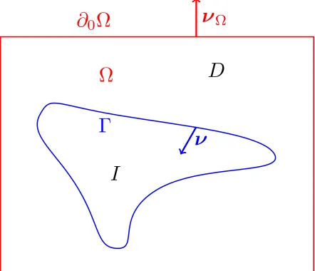
1. Introduction. We start by outlining the mathematical model for receptor-ligand dynamics whose analysis and asymptotic limits will be the main focus of this work. Let Γ be a smooth, compact closed n-dimensional hypersurface contained in the interior of a simply connected domain D _⊂ Rn+1, n = 1,2. The surface Γ

separates the domain D into an interior domain I and an exterior domain Ω. We will denote by∂0Ω the outer boundary of Ω, i.e., the boundary∂D. The vectorsν

and νΩ denote the outward pointing unit normals to Ω on Γ and ∂0Ω, respectively.

Figure 1 shows a cartoon sketch of the setup. We assume that the outer boundary

∂0Ω is Lipschitz. We consider the following problem: Findu: ¯Ω×[0, T)→R+ and

w: Γ_×[0, T)→R+ such that

δΩ∂tu−∆u= 0 in Ω×(0, T), (1.1a)

∇u_·ν=₋1

δk

uw on Γ_×(0, T),

(1.1b)

u=uD or ∇u·νΩ= 0 on∂0Ω×(0, T),

(1.1c)

∗_{Received by the editors December 16, 2015; accepted for publication (in revised form)}

Novem-ber 4, 2016; published electronically February 8, 2017. http://www.siam.org/journals/sima/49-1/M105081.html

Funding: This work was started whilst the authors were participants in the Isaac Newton In-stitute programme: “Free Boundary Problems and Related Topics” and finalized whilst the authors were participants in the Isaac Newton Institute programme: “Coupling Geometric PDEs with Physics for Cell Morphology, Motility and Pattern Formation” supported by EPSRC Grant EP/K032208/1. The work of the first author was partially supported by the Royal Society via a Wolfson Research Merit Award. The work of the second author was funded by the Engineering and Physical Sciences Research Council (EPSRC EP/J004057/1). The work of the third author was supported by the Leverhulme Trust Research Project Grant (RPG-2014-149).

†_{Mathematics Institute, University of Warwick, Coventry, CV4 7AL, UK (C.M.Elliott@warwick.}

ac.uk).

‡_{School of Computing, University of Leeds, Leeds, LS2 9JT, UK ([email protected]).} §_{Mathematical Institute, University of St. Andrews, Fife, KY16 9SS, UK (cv28@st-andrews.}

ac.uk).

360

Fig. 1. A sketch of the cell membraneΓand the extracellular mediumΩ.

∂tw−δΓ∆Γw=∇u·ν on Γ×(0, T), (1.1d)

u(_·,0) =u0₍

·) in Ω,

(1.1e)

w(·,0) =w0(·) on Γ,

(1.1f)

where δΩ, δΓ, δk >0 are given model parameters and the initial data are bounded, nonnegative functions, i.e.,u0_∈L∞_(Ω),w0_∈L∞_{(Γ), andu}0_{, w}0_{≥0. In the above}

∆Γdenotes the Laplace–Beltrami operator on the surface Γ and∆the usual Cartesian

Laplacian inRn+1.

We will use either Dirichlet or Neumann boundary conditions on ∂0Ω. For the Dirichlet case, we assume that the Dirichlet boundary data uD are positive scalar constants. Our analysis remains valid if we consider bounded positive functions for the Dirichlet boundary data; we restrict the discussion to positive scalar boundary data for the sake of simplicity. The restriction to nonnegative solutions is made since we are interested in biological problems whereuandwrepresent chemical concentrations and hence are nonnegative.

Problem (1.1) may be regarded as a basic model for receptor-ligand dynamics in cell biology, modeling the dynamics of mobile cell surface receptors reacting with a mobile bulk ligand, which is a reduction of the model (2.1) presented in section 2. Receptor-ligand interactions and the associated cascades of activation of signalling molecules, so called signalling cascades, are the primary mechanisms by which cells sense and respond to their environment. Such processes therefore constitute a funda-mental part of many basic phenomena in cell biology such as proliferation, motility, the maintenance of structure or form, adhesion, cellular signaling, etc. (Bongrand, 1999; Hynes, 1992; Locksley, Killeen, and Lenardo, 2001). Due to the complexity of the biochemistry involved in signaling networks, an integrated approach combining theoretical and computational mathematical studies with experimental and modeling efforts appears necessary. Motivated by this need, in this work we focus on under-standing a mathematical reduction of theoretical models for receptor-ligand dynamics in cell biology consisting of a coupled system of bulk-surface partial differential equa-tions (PDEs).

A number of recent theoretical and computational studies of receptor-ligand in-teractions (e.g., Marciniak-Czochra and Ptashnyk, 2008; Garc´ıa-Pe˜narrubia, G´alvez, and G´alvez, 2013), employ models which are similar in structure to those considered in this work. Models with similar features arise in the modeling of signaling networks coupling the dynamics of ligands within the cell (e.g., G-proteins) with those on the cell surface (Levine and Rappel, 2005; Jilkine, Mar´ee, and Edelstein-Keshet, 2007; Mori, Jilkine, and Edelstein-Keshet, 2008; R¨atz and R¨oger, 2012, 2014; Madzvamuse, Chung, and Venkataraman, 2015; Bao, Fellner, and Latos, 2014; Morgan and Sharma, 2016). The ability of cells to create their own chemotactic gradients, i.e., to influence the bulk ligand field, has been conjectured to play a crucial role in collective di-rected migration, for example, during neural crest formation (McLennan et al., 2012, 2015a,b) and hence understanding such models is of much biological importance.

Through proving well-posedness results, this work gives a mathematically sound foundation for the use and simulation of coupled bulk-surface models for receptor-ligand dynamics. Moreover, we justify the consideration of various small parameter asymptotic limits of such models, through nondimensionalization using experimentally measured parameter values. We provide a rigorous derivation of the limiting problems and discuss their well-posedness. We also discuss the numerical solution of the original and limiting problems illustrating the asymptotic convergence together with robust and efficient methods for their approximation. This work suggests that models for receptor-ligand dynamics featuring fast reaction kinetics can be derived using classical elements of free boundary methodology as components of the modeling.

While our focus is on receptor-ligand dynamics, problems of a similar structure arise in fields such as ecology where one considers populations consisting of two or more competing species (Holmes et al., 1994). Such a scenario can be modeled by so-called spatial segregation models and the corresponding asymptotic limits have been the subject of much mathematical study (e.g., Conti, Terracini, and Verzini, 2005; Crooks et al., 2004; Dancer et al., 1999). Further details on the cell-biological motivation for studying (1.1), together with the limitsδΩ, δΓ, δk→0, is given in section 2.

The main focus of this work is to show the system of PDEs (1.1) is well-posed and so is meaningful from the mathematical perspective and, furthermore, to obtain reduced models as limits of this system as we send the parameters δΩ, δΓ, and δk to zero. Specifically, we establish existence and uniqueness of a solution to (1.1) and show that in the limits δk → 0, δΩ, δΓ > 0 fixed, δΓ =δk → 0, δΩ > 0 fixed,

δΩ=δΓ =δk → 0, this solution to (1.1) converges to a solution of suitably defined limit problems. Furthermore, in the latter two cases, δΓ =δk → 0 and δΩ =δΓ =

δk→0, the uniqueness of the solution to the limit problems, respectively, constrained parabolic and elliptic problems with dynamic boundary conditions, is also shown. We then show that the limit problems with dynamic boundary conditions may be reformulated as variational inequalities and briefly explore some connections with classical free boundary problems. These reduced models in the form of free boundary problems may be considered as models in their own right and offer simplifications with respect to numerical computation.

That the fast reaction limit (δk →0) leads to interesting free boundary problems is because of the complementary nature of the resulting limit

u_≥0, w_≥0, uw= 0 on Γ.

Such limits have been considered for coupled systems of parabolic equations (posed in the same domain) in a number of previous works (e.g., Evans, 1980; Bothe, 2001; Bothe and Pierre, 2012) with the limiting problem corresponding to a Stefan problem

(Hilhorst, Van Der Hout, and Peletier, 1996; Hilhorst et al., 2001; Hilhorst, Mimura, and Sch¨atzle, 2003). Here in this paper the main complication in the analysis is that the species reside in different domains and the coupling is on the boundary of the bulk domain which results in added technical complications in passing to the limit.

For the limit problemsδΓ=δk = 0 andδΓ=δk=δΩ= 0 with dynamic boundary conditions, we obtain Stefan and Hele–Shaw-type problems on the hypersurface Γ with a differential operator, which may be interpreted as a nonlocal fractional differential operator, obtained by using the Dirichlet to Neumann map for the bulk parabolic and elliptic operators. This leads to an interesting variational inequality reformulation in the case of the limit bulk elliptic equation consisting of a boundary obstacle problem that is satisfied by the integral in time of the solution. The approach follows that employed for the reformulation of the one-phase Stefan problem and the Hele–Shaw problem for which the transformed variable (integral in time of the solution) satis-fies a parabolic (Duvaut, 1973) or elliptic (Elliott, 1980; Elliott and Janovsk`y, 1981) variational inequality, respectively.

Problems related to those considered in this work have been the focus of recent studies. For example, Morgan and Sharma (2016) consider coupled bulk-surface sys-tems of parabolic equations with nonlinear coupling in which the surface resident species are defined on the boundary of the bulk domain. They derive sufficient con-ditions on the coupling to ensure global existence of classical solutions extending the results of Pierre (2010) from the planar case to the coupled bulk-surface case. Schimperna, Segatti, and Zelik (2013) consider the well-posedness of singular heat equation with dynamic boundary conditions of reactive-diffusive type (i.e., including the Laplace–Beltrami of the trace of the solution on the boundary). Bao, Fellner, and Latos (2014) consider a reaction-diffusion equation in a bulk domain coupled to a reaction-diffusion equation posed on the boundary. They prove existence and uniqueness of a weak solution to the problem and establish exponential convergence to equilibrium. V´azquez and Vitillaro (2008, 2009, 2011) study the well-posedness of the Laplace and heat equations with dynamic boundary conditions of reactive and reactive-diffusive type. The heat equation with nonlinear dynamic Neumann bound-ary conditions which arises in problems of boundbound-ary heat control is considered by Athanasopoulos and Caffarelli (2010). The authors prove continuity of the solution and, furthermore, they extend their results to the case where the heat operator in the interior is replaced with a fractional diffusion operator. Existence and uniqueness of weak solutions to Hele–Shaw problems which are Stefan-type free boundary problems with vanishing specific heat are considered by Crowley (1979). Elliptic equations with nonsmooth nonlinear dynamic boundary conditions have been studied in a number of applications. Aitchison, Lacey, and Shillor (1984) propose a simplified model for an electropaint process that consists of an elliptic equation with nonlinear dynamic boundary conditions involving the normal derivative. The authors formally derive the steady state stationary problem which consists of a Signorini problem similar to the elliptic variational inequality we derive in section 9. This problem is studied by Caffarelli and Friedman (1985) where the authors prove that the steady state solution (t_{→ ∞}) of an implicit time discretization solves the Signorini problem proposed as the formal limit by Aitchison, Lacey, and Shillor (1984). A similar problem, which models percolation in gently sloping beaches, that consists of an elliptic equation vari-ational inequality with dynamic boundary conditions involving the normal derivative is proposed and analyzed by Aitchison, Elliott, and Ockendon (1983); Elliott and Friedman (1985); Colli and Kenmochi (1987). Perthame, Quir´os, and V´azquez (2014) derive Hele–Shaw-type free boundary problems as limits of models for tumor growth.

Finally we mention the work of Nochetto, Ot´arola, and Salgado (2015) who consider the numerical approximation of obstacle problems, in particular, they prove optimal convergence rates for the thin obstacle (Signorini) problem and prove quasi-optimal convergence rates for the approximation of the obstacle problem for the fractional Laplacian.

Our main results are stated in Theorems 4.2, 5.3, 6.3, and 7.3.

• In Theorem 4.2 we establish the existence of a unique, bounded solution to (1.1).

• In Theorem 5.3 we present a rigorous derivation that in the limit δk → 0,

δΩ, δΓ >0 fixed, the solution to (1.1) converges to a solution of a system of constrained coupled bulk-surface parabolic equations (cf., (5.1)).

• In Theorem 6.3 we present a rigorous derivation that in the limitδΓ=δk →0, with δΩ >0 fixed, the solution to (1.1) converges to the unique solution of constrained parabolic problem with dynamic boundary condition (cf., (6.1)).

• In Theorem 7.3 we present a rigorous derivation that in the limit δΩ=δΓ =

δk→0, the solution to (1.1) converges to the unique solution of constrained elliptic problem with dynamic boundary condition (cf., (7.1)).

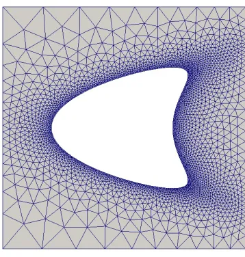
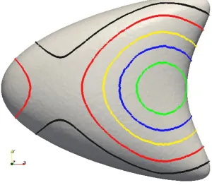
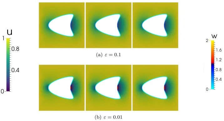
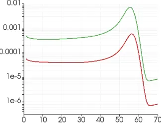
We conclude the paper by providing some numerical experiments employing a coupled bulk-surface finite element method where we support numerically the the-oretical convergence results to a limiting problem and investigate the resulting free boundary problem on a surface.

2. Biological motivation. We now present a model for receptor-ligand dynam-ics and justify, through nondimensionalization of the model using parameter values previously measured in experimental studies, the simplifications and limiting problems considered in this work.

We start with the following model, that corresponds to one of the models pre-sented by Garc´ıa-Pe˜narrubia, G´alvez, and G´alvez (2013) if one neglects the terms involving internalization of receptors and complexes. The reaction under considera-tion is between mobile receptors that reside on the cell surface with ligands present in the extracellular medium (the bulk region surrounding the cell). We assume a single species of mobile surface (cell membrane) resident receptor whose concentration (sur-face density) is denoted bycr and a single species of bulk resident diffusible ligand whose concentration (bulk concentration) is denoted bycL. The receptor and ligand react reversibly on the surface to form a (surface resident, mobile) receptor-ligand complex, whose concentration is denoted bycrl. The kinetic constants kon and koff represent the forward and reverse reaction rates. Denoting by Γ the cell surface and by Ω the extracellular medium with outer boundary ∂0Ω (cf., Figure 1), we have in mind models of the following form:

∂tcL−DL∆cL= 0 in Ω×(0, T), (2.1a)

DL∇cL·ν=−koncLcr+koffcrl on Γ×(0, T), (2.1b)

cL=cD orDL∇cL·νΩ= 0 on∂0Ω×(0, T),

(2.1c)

∂tcr−Dr∆Γcr=−koncLcr+koffcrl on Γ×(0, T), (2.1d)

∂tcrl−Drl∆Γcrl=koncLcr−koffcrl on Γ×(0, T). (2.1e)

The model is closed by suitable (bounded, nonnegative) initial conditions. For the outer boundary condition we take either a Dirichlet or a Neumann boundary condition. The Dirichlet boundary condition, withcD >0 a positive constant, arises under the modeling assumption that the background concentration of ligands sufficiently far

away from the cell is uniform. Alternatively, the Neumann boundary condition arises from assuming zero flux across∂0Ω.

2.1. Nondimensionalization and limit problems. We are interested in dif-ferent limit problems arising from model (2.1) for ligand-receptor binding. To simplify notation, we write the unknowns asu=cL, w=cr, and χ=crl and the parameters

DΩ=DL,DΓ =Dr=Drl,k=kon,k−1=koff.

The first problem we consider is to findu: Ω_×[0, T)_→Randw, χ: Γ×[0, T)→R

such that

∂tu−DΩ∆u= 0 in Ω×(0, T), (2.2a)

DΩ_∇u_·ν=₋kuw+k−1χ on Γ×(0, T), (2.2b)

u=uD orDΩ∇u·νΩ= 0 on∂0Ω×(0, T),

(2.2c)

∂tw−DΓ∆Γw=DΩ∇u·ν on Γ×(0, T), (2.2d)

∂tχ−DΓ∆Γχ=−DΩ∇u·ν on Γ×(0, T),

(2.2e)

u(·,0) =u0(·) in Ω,

(2.2f)

w(·,0) =w0(·) on Γ,

(2.2g)

χ(_·,0) =χ0(_·) on Γ.

(2.2h)

In order to determine the sizes of each coefficient, we take the following rescaling. We set

˜

x=x/L, t˜=t/S, u˜=u/U, w˜=w/W, χ˜=χ/X,

where Lis a length scale,S is a time scale, U, W. andX are typical concentrations foru, w, andχ, respectively.

Applying the chain rule, this leads to a nondimensional form of (2.2):

δΩ∂˜tu˜−∆˜u= 0 in ˜Ω×(0,T˜), (2.3a)

∇u˜_·ν=₋1

δk ˜

uw˜+δχχ˜ on ˜Γ×(0,T˜), (2.3b)

˜

u= ˜uD or ∇u˜·ν_Ω˜ = 0 on∂0Ω˜ ×(0,T˜),

(2.3c)

∂˜tw˜−δΓ∆Γ˜w˜=µ∇u˜·ν on ˜Γ×(0,T˜),

(2.3d)

∂˜tχ˜−δΓ∆˜Γχ˜=−µ0∇u˜·ν on ˜Γ×(0,T˜),

(2.3e)

˜

u(·,0) = ˜u0(·) :=u0(·)/U in Ω,

(2.3f)

˜

w(_·,0) = ˜w0(_·) :=w0(_·)/W on Γ,

(2.3g)

˜

χ(_·,0) = ˜χ0(_·) :=χ0(_·)/X on Γ.

(2.3h)

Here we have six nondimensional coefficients:

δΩ= L

2

DΩS, δk= DΩ

kLW, δχ =

k−1LX

DLU

, δΓ= DΓS

L2 ,

µ=DΩSU

LW , µ

0 ₌DΩSU

LX .

Taking values from Table 1, we infer that

δΩ= (5.6 s)_·S−1, δk= 5.7·10−2, δχ = 8.7·10−2,

δΓ= (1.8_·10−4s−1)_·S, µ= (5.7_·10−2s−1)_·S, µ0= (5.7_·10−2s−1)_·S.

Table 1

Parameters used for rescaling equations. The values for U and W are extreme values taken from within a physical range fromGarc´ıa-Pe˜narrubia, G´alvez, and G´alvez (2013).

Parameter Value Source

L 7.5·10−6_{m Garc´ıa-Pe˜narrubia, G´alvez, and G´alvez (2013)}

U 1.0·10−3_{mol m}−3 _{Garc´ıa-Pe˜narrubia, G´alvez, and G´alvez (2013)}

W 2.3·10−8_{mol m}−2 _{Garc´ıa-Pe˜narrubia, G´alvez, and G´alvez (2013)}

X 2.3·10−8_{mol m}−2 _{Limited by total receptor concentration}

DΩ 1.0·10−11m2s−1 Linderman and Lauffenburger (1986)

DΓ 1.0·10−15m2s−1 Linderman and Lauffenburger (1986)

kon 1.0·103m3mol−1s−1 Garc´ıa-Pe˜narrubia, G´alvez, and G´alvez (2013)

koff 5.0·10−3s−1 Garc´ıa-Pe˜narrubia, G´alvez, and G´alvez (2013)

First, we note thatδχ 1. Considering the limitδχ→0 by dropping the terms

δχχ decouples the equations for ˜u,w˜, from the equation for ˜χ. This results in the problem, which we have written in terms of the original variables:

∂tu−δ_Ω−1∆u= 0 in Ω, (2.4a)

∇u_·ν=₋1

δk

uw on Γ_×(0, T),

(2.4b)

u=uD or∇u·νΩ= 0 on∂0Ω,

(2.4c)

∂tw−δΓ∆Γw=µ∇u·ν on Γ,

(2.4d)

u(_·,0) =u0(_·) in Ω,

(2.4e)

w(_·,0) =w0(_·) on Γ.

(2.4f)

This is the first problem we consider in section 4. Similar methods to those shown in the remaining sections can be used to show well-posedness of the system (2.3) and rigorously take the limit δχ → 0 for δk, δΩ, δΓ, µ > 0 fixed. The existence and uniqueness theory of (2.3) and the limit to obtain (2.4) in the more general case of time dependent domains are considered by Alphonse, Elliott, and Terra (2016).

We see that δk 1. Again using the original variables, we consider the limit problem: Findu: Ω_×[0, T)→Randw: Γ×[0, T)→Rsuch that

∂tu−δΩ−1∆u= 0 in Ω,

(2.5a)

uw= 0 on Γ,

(2.5b)

u=uD or∇u·νΩ= 0 on∂0Ω,

(2.5c)

∂tw−δΓ∆Γw=µ∇u·ν on Γ,

(2.5d)

u(_·,0) =u0(_·) in Ω,

(2.5e)

w(_·,0) =w0₍

·) on Γ,

(2.5f)

where δΩ, δΓ, and µ are positive parameters. We consider this problem as a large ligand–receptor binding rate limit of (2.2). We consider the well posedness of the problem and the justification of the limit in section 5.

We can consider different problems by choosing different timescales S. We can achieve two different problems by resolving the timescale of the volumetric diffusion (δΩ_≈1) or the timescale of the surface adsorption flux (µ_≈1).

ForS=L2_{/DΩ= 5.6 s, we have}

δΩ= 1, δΓ = 1.0_·10−31, µ= 3.2_·10−1_≈1.

This leads to a parabolic limit problem with dynamic boundary condition: Find

u: Ω_×[0, T)_→Randw: Γ×[0, T)→Rsuch that

∂tu−δ_Ω−1∆u= 0 in Ω, (2.6a)

uw= 0 on Γ,

(2.6b)

u=uD on∂0Ω,

(2.6c)

∂tw=∇u·ν on Γ, (2.6d)

u(·,0) =u0(·) in Ω,

(2.6e)

w(·,0) =w0(·) on Γ.

(2.6f)

In this case, we have resolved the timescale of the diffusion of ligand, but the effect of the diffusion of surface bound receptor is lost. We consider the well-posedness of this problem and the justification of the limit in section 6.

Alternatively, takingS= 102_{s, we have}

δΩ= 5.7_·10−21, δΓ= 1.8_·10−21, µ= 5.7_≈1.

This leads to an elliptic problem with dynamic boundary condition: Find u: Ω_× [0, T)→Randw: Γ×[0, T)→Rsuch that

−∆u= 0 in Ω,

(2.7a)

uw= 0 on Γ,

(2.7b)

u=uD on∂0Ω,

(2.7c)

∂tw=∇u·ν on Γ, (2.7d)

w(_·,0) =w0(_·) on Γ.

(2.7e)

In this regime, we have chosen a timescale so that the diffusion of ligand has no memory of its previous value, except via the boundary condition. This means this problem no longer requires an initial condition for uto be a closed system. We do not consider the exterior Neumann boundary condition in this case, since we arrive at a trivial problem where the solution isu= 0 and w=w0. The well-posedness of this problem and a rigorous justification of limit is given in section 7. We also show in section 9 that we can reformulate problems (2.6) and (2.7) by integrating forwards in time to derive variational inequalities.

Remark 2.1. In the large ligand-receptor binding rate limit, the nonlinear con-straint (2.5b) (uw= 0) implies that the domain Γ is separated into two regions, for positive times, where u= 0 and where u >0. In the region u >0, we have a Neu-mann boundary condition_∇u_·ν= 0. This can be interpreted that there is no flux of ligand onto or off the surface in this region. In the regionu= 0, we have a Dirichlet boundary condition (u= 0). This can be interpreted that the ligand in this region is perfectly (i.e., instantaneously) absorbed.

3. Preliminaries. In this section, we define some of our notation and collect some technical results that will be used in the subsequent sections. We also prove some compact embedding results in Lemmas 3.6, 3.7, and 3.8 that are used to deduce strong convergence from weak convergence in suitable spaces.

Given a Hilbert space Y we denote the dual space of linear functionals onY by (Y)0. As we consider functions defined on surfaces, along with the surface function spacesL2_{(Γ) andH}1_{(Γ), we will also use the spaceH}1/2_{(Γ) and its dual (H}1/2_(Γ))0_.

For a Hilbert spaceY, we consistently use the notation _h·,_·iY to denote the duality pairing between the spaceY and its dual (Y)0.

Definition 3.1. The space H1/2(Γ) is defined by

(3.1) H1/2(Γ) :=nξ∈L2(Γ) :kξkH1/2_(Γ)<+∞ o

,

where

(3.2) _kξ_kH1/2_(Γ):= Z

Γ

ξ2 dσ+

Z

Γ

Z

Γ

|ξ(x)−ξ(y)|2

|x₋y_|n dσ(x) dσ(y) !12

.

The space can be characterized via the following result.

Proposition 3.2 (trace theorem).The trace operator from H1(Ω)toH1/2(Γ)is bounded and surjective.

Proof. The result can be found in (Grisvard, 2011, Thm 1.5.1.3).

We recall the following interpolated trace inequality.

Proposition 3.3 (interpolated trace theorem). For all φ∈H1(Ω) and for any δ >0

(3.3) _kφ_k2_L2_(Γ)≤δk∇φk

2

L2_(Ω)+cδkφk2_L2_(Ω).

Proof. See, e.g., (Grisvard, 2011, Thm 1.5.1.10).

Note that forξ_∈L2_{(Γ) andρ}

∈H1/2_{(Γ) the following duality pairing is equal to}

theL2_{(Γ) inner-product:}

(3.4) hξ, ρiH1/2_(Γ)=

Z

Γ ξρ dσ.

3.1. Compact embeddings. Since we are dealing with nonlinear problems, we will need to use some compact embeddings of Bochner spaces.

We recall that if {fk} is a sequence of bounded functions inLp(0, T;B) withB a Banach space, for 1≤p < ∞, then there exists a subsequence{fkj} ⊂ {fk} and

f ∈Lp_{(0, T;B) such that}

(3.5) fkj * f in L

p

(0, T;B).

Here we are interested to show under what conditions we may assert the existence of a strongly convergent subsequence. The basic results we require are summarized by Simon (1986).

Lemma 3.4 (Aubin–Lions–Simons compactness theory (Simon, 1986)). Let{fk}

be a bounded sequence of functions in Lp_{(0, T;B), where B is a Banach space and} 1_≤p_{≤ ∞}. If

1. the sequence of functions _{fk} is bounded in Lp(0, T;X), where X is

com-pactly embedded in B,

2. and either

(a) the derivatives_{∂tfk}are bounded in the spaceLp(0, T;Y), whereB ⊂Y

or

(b) for eachk, the time translates of{fk} are such that

(3.6)

Z T−τ

0

fk(t+τ)−fk(t) p

B dt→0 as τ→0,

then there exists a subsequence_{fkj} ⊂ {fk} andf ∈L

p_{(0, T;X)such that}

(3.7) fkj * f inL

p_{(0, T;X),}

fkj →f inL

p_{(0, T;B).}

Remark 3.5. Using the criterion 2(a), we see that if_{ηk} ⊂L2(0, T;L2(Ω)) with a constantC >0 such that

kηkkL2_(0,T;H1_(Ω))+k∂tηkk_L2_0,T;(H1_(Ω))0≤C for allk,

then, there exists a subsequence, for which will use the same subscript {ηk}, and

η∈L2_{(0, T;H}1_{(Ω)) such that}

(3.8) ηk * η inL

2_{(0, T;H}1_(Ω)),

ηk →η inL2(0, T;L2(Ω)).

This follows from the compact embedding ofH1_{(Ω) inL}2_(Ω).

However, we wish to recover strong convergence of a subsequence with less control over the time derivatives. The generality of criterion 2(b) allows a more general weak in time notion of solution to be used.

We will apply this result for sequences to derive strongly convergent subsequences inL2(0, T; (H1/2_(Γ))0_).

Lemma 3.6. Let {ξk} be a bounded sequence in H1/2(Γ). Then there exists a

subsequence _{ξkj} ⊂ {ξk} andξ∈H

1/2_{(Γ)such that}

(3.9) ξkj * ξ inH

1/2_(Γ),

ξkj →ξ inL

2_(Γ).

Proof. For anyρ_∈H1/2_{(Γ), we define an extension to Ω, written Eρ}

∈H1_(Ω),

as the unique solution of:

−∆(Eρ) = 0 in Ω,

Eρ= 0 on∂0Ω,

Eρ=ρ on Γ.

We note that for a constant independent ofρ, we have

kEρkH1_(Ω)≤ckρk_H1/2_(Γ).

This implies we have a sequence _{Eξk} which is uniformly bounded in H1(Ω): There existsC0>0 such that

kEξkkH1_(Ω)≤C0.

From the compact embedding of H1_{(Ω) into L}2_{(Ω), we know that there exists a}

subsequence_{ξkj} ⊂ {ξk}andη ∈H

1_{(Ω) such that}

Eξkj →η inL

2_(Ω).

Denoteξ=η_|Γ. Fixε >0 and chooseδ≤ε/(4C0). From the strong convergence

of_{Eξkj}, we know there existsKsuch that forj ≥K,

Eξkj −η

_L2_(Ω)≤

ε

2cδ

,

wherecδ is from Proposition 3.3. It follows that for j≥K, we can infer by applying the interpolated trace inequality (Proposition 3.3), withδas above, that

ξkj−ξ

_L2_(Γ)≤δ

Eξkj−η

_H1_(Ω)+cδ

Eξkj−Eξ

_L2_(Ω)

≤2δC0+ε 2 ≤ε.

Thus, we have shown the strong convergence ofξk toξin L2(Γ).

Lemma 3.7. Let {ξk} be a bounded sequence in L2(Γ). Then there exists a

sub-sequence _{ξkj} ⊂ {ξk} andξ∈L

2_{(Γ) such that}

(3.10)

ξkj * ξ inL

2_(Γ),

ξkj →ξ in

H1/2_(Γ)0_.

Proof. Since {ξk} is uniformly bounded in L2(Γ), we know that it has a sub-sequence {ξkj} which weakly converges to some ξ ∈ L

2_{(Γ). We suppose, for}

con-tradiction, that there exists no subsequence of{ξkj} that strongly converges toξ in

(H1/2_(Γ))0_{. This implies that there existsδ >0 such that}

ξkj−ξ

_(H1/2_(Γ))0 ≥δ.

Using the definition of (H1/2_(Γ))0 _{as the dual space to H}1/2_{(Γ), this implies there}

exists a sequence{ρj} ⊂H1/2(Γ) with ρj

_H1/2_(Γ)= 1, such that for allj

hξkj −ξ, ρjiH1/2_(Γ)= Z

Γ

(ξkj −ξ)ρj dσ≥

δ

2.

From Lemma 3.6, we know that a subsequence _{ρjl} ⊂ {ρj} converges strongly to

ρ∈H1/2_{(Γ) in L}2_{(Γ). Hence, we can infer}

Z

Γ

(ξkj−ξ)ρ dσ≥

δ

2.

However, this contradicts the supposition that ξkj converges weakly to ξ in

L2_(Γ).

We conclude this section with a result which is similar in nature to the previous results.

Lemma 3.8. Let {ηk} be a bounded sequence in L2(0, T;H1(Ω)) and η ∈

L2_{(0, T;H}1_{(Ω))such that}

(3.11) ηk →η inL2(0, T;L2(Ω)).

Then the trace sequence converges to the trace of the limit:

ηk|Γ →η|Γ inL2(0, T;L2(Γ)).

(3.12)

Proof. Denote byC0>0 the upper bound of_{ηk} andη inL2(0, T;H1(Ω)):

kηkk_L2_(0,T;H1_(Ω))+kηk_L2_(0,T;H1_(Ω))≤C0.

Fix ε > 0 and choose δ _≤ ε/(2C0). Then from the convergence of _{ηk} in

L2_{(0, T;L}2_{(Ω)), there existsK such that fork}

≥K,

kηk−ηkL2_(0,T;L2_(Ω))≤

ε

2cδ

,

wherecδ is from Proposition 3.3. It follows that fork≥K, we can infer by applying the interpolated trace inequality (Proposition 3.3), withδas above, that

kηk−ηk_L2_(0,T;L2_(Γ))≤δkηk−ηk_L2_(0,T;H1_(Ω))+cδkηk−ηk_L2_(0,T;L2_(Ω))

≤δC0+ε 2 ≤ε.

Thus, we have shown the strong convergence ofηk toη inL2(0, T;L2(Γ)).

4. Ligand-receptor model. In this section, we establish an existence and uniqueness theory for (1.1). As described in section 2.1, (1.1) arises from (2.1) if one neglects the receptor-ligand complexes, nondimensionalizes as in (2.3), and (for simplicity) sets the surface interchange fluxµ= 1.

In order to introduce the concept of a weak solution to (1.1), for γ _∈ R, we

introduce the Sobolev space

He1γ(Ω) :={v∈H

1_(Ω)

|v=γ on∂0Ω_},

where the boundary values are understood in the sense of traces and we adopt the notation of using the same symbol for a function and its trace. We now introduce our concept of a weak solution to (1.1).

Definition 4.1 (weak solution of (1.1)). For the Dirichlet boundary data case, we say that a pair (u, w) ∈ L2_{(0, T;H}1

e_uD(Ω))×L2(0, T;H1(Γ)) with u, w ≥ 0 and

with (∂tu, ∂tw)∈L2(0, T; (He01(Ω))0)×L2(0, T; (H1(Γ))0) is a weak solution of (1.1)

if for all (η, ρ)_∈H1

e0(Ω)×H1(Γ) and for a.e.t∈(0, T)

δΩ_h∂tu, ηi_H1

e₀(Ω)+

Z

Ω∇

u_{· ∇}η dx=₋1

δk Z

Γ

uwη dσ,

(4.1a)

h∂tw, ρi_H1_(Γ)+δΓ Z

Γ∇

Γw_{· ∇}Γρ dσ=₋1

δk Z

Γ

uwρ dσ.

(4.1b)

In the case of Neumann boundary data, we say that a pair(u, w)_∈L2_{(0, T;H}1_(Ω))

×

L2_{(0, T;H}1_{(Γ)) with u, w}

≥ 0 and with (∂tu, ∂tw) ∈ L2(0, T,(H1(Ω))0) ×

L2_{(0, T; (H}1_(Γ))0_{) is a weak solution of (1.1) if for all (η, ρ)}

∈H1_(Ω)

×H1_{(Γ) and} for a.e.t_∈(0, T)

δΩh∂tu, ηiH1_(Ω)+ Z

Ω∇

u· ∇η dx=−_δ1

k Z

Γ

uwη dσ,

(4.2a)

h∂tw, ρiH1_(Γ)+δΓ Z

Γ∇

Γw· ∇Γρ dσ=−_δ1

k Z

Γ

uwρ dσ.

(4.2b)

We note that if u _∈ L2_{(0, T;H}1_{(Ω)) then by the trace theorem u}

∈

L2_{(0, T;H}1/2_{(Γ)). We now show the well-posedness of problem (1.1) in the sense}

of the following theorem.

Theorem 4.2 (existence and uniqueness of a bounded solution pair to (1.1)). Given bounded, nonnegative initial datau0 andw0, there exists a unique solution pair

(u, w) to the systems (4.1) and (4.2). Furthermore, we have that in the case of Dirichlet data

(4.3) 0≤u(x, t)≤max(ku0kL∞(Ω), uD) for a.e. (x, t)∈Ω×(0, T), 0≤w(x, t)≤ kw0kL∞_(Γ) for a.e. (x, t)∈Γ×(0, T),

or in the case of Neumann data

(4.4) 0≤u(x, t)≤ ku0kL∞(Ω) for a.e. (x, t)∈Ω×(0, T), 0_≤w(x, t)_{≤ k}w0_kL∞_(Γ) for a.e. (x, t)∈Γ×(0, T).

Proof. In the interests of brevity we give the full details of the proof only in the Dirichlet case. An analogous argument holds for the case of Neumann boundary conditions.

We start by replacingwbyM(w) in the nonlinear coupling terms, whereM: R→ R+ is the cutoff function

(4.5) M(r) =



  

  

0, r <0, r, 0_≤r_≤M, M, r > M

withM _{≥ k}w0_kL∞_(Γ). This leads us to consider the following problem. Find (u, w),

in the same spaces as Definition 4.1, that satisfy for all (η, ρ)_∈H1

e0(Ω)×H

1_{(Γ) and}

for a.e. t_∈(0, T)

δΩ_h∂tu, ηiH1 0(Ω)+

Z

Ω∇

u_{· ∇}η dx=₋1

δk Z

Γ

uM(w)η dσ,

(4.6)

h∂tw, ρiH1_(Γ)+δΓ Z

Γ∇

Γw· ∇Γρ dσ=−1 δk

Z

Γ

uM(w)ρ dσ.

(4.7)

As M(w) is bounded, existence for this problem with the cutoff nonlinearity can be shown via a Galerkin method and standard energy arguments. We now show positivity of the solutions to (4.6), (4.7): u, w_≥0 a.e. in their domains and that the trace of u _≥ 0 on Γ . Testing (4.6) with u− = min(u,0) and using the fact that

M(w)_≥0, we have

δΩ

2

d dt

Z

Ω

(u−)2 dx+ Z

Ω|∇

(u−)|2 dx=−1

δk Z

Γ

(u−)2M(w) dσ≤0.

Since u0 _≥ 0, we have u_≥ 0 a.e. in Ω_×(0, T). Moreover, by the trace inequality, applied to u−, we have that the trace of u is nonnegative. We next test (4.7) with

w−= min(w,0) to get

1 2

d dt

Z

Γ

(w−)2 dσ+δΓ Z

Γ|∇

Γ(w−)|2 dσ=−1

δk Z

Γ

uM(w)w− dσ= 0,

as M(w)w− = 0 from the definition ofM() (4.5). Since w0 ≥0, we see thatw≥0 a.e. in Γ_×(0, T). We now show pointwise bounds. Let (u, w) be solutions of (4.6) and (4.7) and setθw_{= (w}

− kw0_kL∞_(Γ)). The variable θw satisfies

h∂tθw, ρiH1_(Γ)+δΓ Z

Γ∇ Γθw

· ∇Γρ dσ=−1 δk

Z

Γ

uwρ dσ.

We test withρ= (θw₎

+≥0 and recall that whenu, w≥0 then

1 2 d dt Z Γ

(θw

+)2 dσ+δΓ

Z

Γ|∇ θw

+|2 dσ=−

1

δk Z

Γ uwθw

+ dσ≤0.

This implies thatθw

+ = 0 and hencew≤ kw0kL∞_(Γ). The same argument for uwith

θu _{= (u}

−max(uD,kuk_L∞_(Ω)) so that θu₊ ∈ H_e01, gives u≤max(uD,kuk_L∞_(Ω)). As

M was chosen such thatM _{≥ k}w0_kL∞_(Γ)andw≥0, we have thatM(w) =w, hence

we have constructed a solution to (4.1) which satisfies

(4.8) 0_≤u_≤max(_ku0_k∞, uD) and 0≤w≤ kw0k∞.

It remains to show that the solution is unique. To do this, we argue as follows. Let (u1, w1) and (u2, w2) be two (weak) solutions of (4.1) . Definingeu _:=u1

−u2

and ew_:=w1

−w2 we have that eu_{, e}w _{satisfy for all (η, ρ)}

∈H1

e0(Ω)×H1(Γ) and for a.e.t∈(0, T)

δΩ_h∂teu, ηi_H1

e₀(Ω)+

Z

Ω∇ eu

· ∇η dx=₋1

δk Z

Γ

(u1w1₋u2w2)η dσ,

(4.9a)

h∂tew, ρiH1_(Γ) dσ+ Z

Γ

δΓ_∇Γew

· ∇Γρ dσ=₋1

δk Z

Γ

(u1w1₋u2w2)ρ dσ.

(4.9b)

Let ψ : R → R be a smooth convex function satisfying ψ(0) =ψ0(0) = 0. Setting

η=ψ0_(eu_{) andρ=ψ}0_(ew_{) in (4.9) and combining the equations gives}

d dt

Z

Ω

δΩψ(eu_{) dx+} Z

Γ

ψ(ew_{) dσ}

+

Z

Ω ψ00(eu₎

|∇eu

|2 dx+

Z

Γ

δΓψ00(ew₎

|∇Γew

|2 dσ

(4.10)

=₋1

δk Z

Γ

(u1w1₋u2w2) ψ0_(eu_{) +ψ}0_(ew₎

dσ.

Hence asψis convex we have

d dt

Z

Ω

δΩψ(eu_{) dx+} Z

Γ

ψ(ew_{) dσ}

≤ −_δ1

k Z

Γ

(u1w1−u2w2) ψ0(eu_{) +ψ}0_(ew₎

dσ.

(4.11)

Integration in time gives

(4.12)

Z

Ω

δΩψ(eu₍

·, t)) dx+

Z

Γ ψ(ew₍

·, t)) dσ

≤ −_δ1

k Z t

0

Z

Γ

(u1w1₋u2w2) ψ0_(eu_{) +ψ}0_(ew₎

dσ dt,

as eu₍

·,0) = 0 and ew₍

·,0) = 0 and we have chosen ψ such thatψ(0) = 0. Defining the function

sgn(η) =

      

1 ifη >0,

0 ifη= 0,

−1 ifη <0,

we replaceψby a sequence of smooth functionsψk such that

ψk(x)→ |x|, ψk0(x)→sgn(x), x∈R,

pointwise and pass to the limit (k_{→ ∞}), which yields

(4.13)

Z

Ω δΩ

e u

(·, t) dx+

Z

Γ

e

w (·, t)

dσ

≤ −_δ1

k Z t

0

Z

Γ

(u1w1₋u2w2) sgn(eu_{) + sgn(e}w₎

dσ dt.

Fora1, b1, a2, b2_∈R+ it is easily verified that

(a1b1−a2b2)(sgn(a1−a2) + sgn(b1−b2))≥0,

hence the right-hand side of (4.13) is nonpositive. Thus for a.e.,t∈(0, T)

Z

Ω δΩ_|eu

| dx+

Z

Γ| ew

| dσ

= 0,

which completes the proof of uniqueness and hence the proof of the theorem.

In the subsequent sections we will consider the limit problems obtained on sending

δΩ, δΓ, and δk to zero in (1.1). To this end we derive some estimates on the solution pair (u, w) of (4.1) , which we will use in the subsequent sections to deduce the exis-tence of convergent subsequences which converge to solutions of the limit problems. We note that the bounds hold for constants which are independent ofδk, δΓ, andδΩ.

Lemma 4.3 (estimates for the solution of (4.1) and (4.2)). The solution pair

(u, w)to(4.1)and(4.2)satisfy the following estimates,

δΩkuk2L∞_((0,T);L2_(Ω))+ 2k∇uk

2

L2_((0,T);L2_(Ω))≤δΩ Z

Ω

u20 dx+CD,

kwk2L∞_((0,T);L2_(Γ))+ 2δΓk∇Γwk

2

L2_((0,T);L2_(Γ))≤ Z

Γ w20 dσ,

(4.14)

where CD ∈ R+ depends on the Dirichlet boundary data uD and CD = 0 in the

case of the Neumann boundary condition. Furthermore, we have an estimate on the nonlinearity:

1

δk k

uwkL1_((0,T)×Γ)≤ kw0k_L1_(Γ). (4.15)

The following estimate on time translates of u andw along with Lemma 3.4 will be used to deduce the necessary compactness

(4.16)

δΩ

Z T−τ

0

Z

Ω

u(·, t+τ)−u(·, t)2

dx dt

+

Z T−τ

0

Z

Γ

w(_·, t+τ)₋w(_·, t)2

dσ dt_≤Cτ,

where the constant C is independent ofτ, δΩ, δΓ, andδk.

Proof. The first estimate (4.14) follows from a straightforward energy argument due to the nonnegativity of uand w. Specifically, test with (u₋Du, w), where Du

satisfies∆Du= 0 in Ω,Du= 0 on Γ, andDu=uDon∂0Ω in the Dirichlet case (4.1) or simply with (u, w) in the Neumann case (4.2).

For the estimate (4.15) we have, using the nonnegativity ofu, w,

1

δk k

uwkL1_(Γ×(0,T)) = 1 δk Z T 0 Z Γ

wu dσ dt

=

Z T

0

Z

Γ−

∂tw dσ dt

=

Z

Γ−

w(_·, T) +w0(_·) dσ

≤ w

0 _L1_(Γ),

where we have used the nonnegativity ofwin the last step.

For the estimate (4.16) we argue as follows. For a fixed τ ∈ (0, T) and for

t∈[0, T −τ) introducing the notation ¯∂τf(t) :=f(t+τ)−f(t) we have, using (4.1),

Z

Γ

w(·, t+τ)−w(·, t)2

dσ = Z τ 0 Z Γ

∂tw(·, t+s) ¯∂τw(·, t) dσ ds

=

Z τ

0

Z

Γ−

δΓ_∇Γw(_·, t+s)_{· ∇}Γ∂¯τw(·, t)− 1

δk

[uw](_·, t+s) ¯∂τw(·, t) dσ ds.

Integrating in time gives

Z T−τ

0

Z

Γ

w(_·, t+τ)₋w(_·, t)2

dσ dt

(4.17)

=

Z τ

0

Z T−τ

0

Z

Γ−

δΓ∇Γw(·, t+s)· ∇Γ∂¯τw(·, t)

−_δ1

k

[uw](·, t+s) ¯∂τw(·, t) dσ dt ds

≤ Z τ

0

2δΓ_k∇Γw_k2_L2_(Γ×(0,T))+ ∂¯τw

_L∞_(Γ×(0,T))

1

δkk

uw_kL1_(Γ×(0,T)) ds,

where we have used Young’s inequality in the last step. Applying the estimates (4.8), (4.14), and (4.15) in (4.17) yields the desired estimate for the second term in (4.16). For the bound on the first term in (4.16), we note that as ¯∂τu∈He01(Ω),

δΩ

Z

Ω

¯

∂τu(·, t)2 dx

=

Z τ

0

Z

Ω−∇

u(_·, t+s)_{· ∇}∂¯τu(·, t)− 1

δk

[uw](_·, t+s) ¯∂τu(·, t) dσ ds,

from which the desired bound follows from an analogous calculation to (4.17) together with the estimates (4.8), (4.14), and (4.15).

5. Fast reaction limit problem (δk = 0). We now show that for fixed δΩ, δΓ > 0 as δk → 0 the solution to (1.1) converges to a (weak) solution to the following constrained parabolic limit problem. For convenience we work withv=₋w

and setv0₌

−w0_.

Fig. 2.Sketch of the functionβ; cf.(5.2).

Problem 5.1 (problem for instantaneous reaction rate). Find u¯: Ω×[0, T)→

R+,¯v: Γ×[0, T)→R− such that

δΩ∂tu¯−∆¯u= 0 in Ω×(0, T), (5.1a)

∇u¯_·ν+∂tv¯−δΓ∆Γ¯v= 0 and v¯∈β(¯u) on Γ×(0, T),

(5.1b)

¯

u=uD or ∇u¯·νΩ= 0 on ∂0Ω×(0, T),

(5.1c)

¯

u(_·,0) =u0(_·)_≥0 in Ω,

(5.1d)

¯

v(_·,0) =v0(_·)_≤0 on Γ.

(5.1e)

Here β:R→ {0,1}R is the set valued function (cf. Figure2)

(5.2) β(r) =



  

  

∅ ifr <0,

[_−∞,0] ifr= 0,

{0_} ifr >0.

We consider (5.1) as a parabolic equation with dynamic boundary conditions inter-preted as a differential inclusion.

In order to define a weak solution to (5.1) we define the Bochner spaces

Ve0(Ω) = (

v_∈L2_{0, T;H}1

e0(Ω)

:∂tv∈L2

0, T;H1

e0(Ω) 0

)

and

V(Γ) =

(

v_∈L20, T;H1(Γ):∂tv∈L2

0, T;H1(Γ)0

)

.

We will make use of the following function space

Ve0(Ω,Γ) := (

v∈ Ve0(Ω) :v|Γ∈ V(Γ) )

.

We note that similar spaces have been introduced for the weak formulation of a parabolic problems with dynamic boundary conditions, (see, for example, Calatroni and Colli, 2013).

Definition 5.2 (weak solution of Problem 5.1). We say that a pair(¯u,v¯)with u_∈L2_{(0, T;H}1

e_uD(Ω))∩L∞(0, T;L2(Ω)) and ¯v∈L2(0, T;H1(Γ))∩L∞(0, T;L2(Γ))

with u¯≥0 andv¯≤0 is a weak solution of Problem5.1 if for allη ∈ Ve0(Ω,Γ)with

η(·, T) = 0, we have

(5.3)

Z T

0 −

δΩh∂tη,u¯iH1

euD(Ω)+

Z

Ω∇

¯

u· ∇η dx− h∂tη,v¯iH1_(Γ)

+

Z

Γ

δΓ∇Γ¯v· ∇Γη dσ

!

dt=

Z

Ω

δΩu0η(·,0) dx+

Z

Γ

v0η(·,0) dσ

and

¯

v_∈β(¯u) a.e. on Γ_×(0, T).

(5.4)

We make the corresponding modifications to the function spaces for the Neumann boundary condition.

Theorem 5.3 (convergence of the solution of (1.1) to a solution of (5.1)). As δk → 0 the solution pair (u, w) to (4.1) converge (up to a subsequence) to a pair (¯u,w¯)in the following topologies:

u *u¯ inL2_{(0, T;H}1

e_uD(Ω)) (5.5)

(u *u¯ inL2(0, T;H1(Ω)) in the Neumann case), w *w¯ inL2_{(0, T;H}1_(Γ)),

(5.6)

u→u¯ inL2(Ω×(0, T)),

(5.7)

w_→w¯ inL2(Γ_×(0, T)).

(5.8)

Moreover, the pair(¯u,¯v), with ¯v=₋w¯ are a weak solution to Problem5.1.

Proof. In the interests of brevity we give the details for the Dirichlet boundary condition case. The Neumann case is handled similarly.

From standard weak compactness arguments (3.5) together with the estimate (4.14), we can extract a subsequence which we will still denote (u, w) such that

u *u¯ inL2(0, T;He1_uD(Ω)),

w *w¯ in L2(0, T;H1(Γ)).

From the Aubin–Lions–Simon compactness theory (Lemma 3.4), the estimate on time translates (4.16) means we can extract a subsequence which we will still denote (u, w) such that

u→u¯ inL2(Ω×(0, T)), w_→w¯ in L2(Γ_×(0, T)).

We now show the pair (¯u,¯v), with ¯v=₋w¯, are a weak solution to Problem 5.1. We start by noting that for allη_{∈ V}e0(Ω,Γ) withη(·, T) = 0, we have

Z T

0 −

δΩ_h∂tη, ui_H1

euD(Ω)+

Z

Ω∇

u_·∇η dx dt₋δΩ

Z

Ω

u0η(_·,0) dx=

Z T 0 Z Γ− 1 δk

uwη dσ dt

=

Z T

0 − h

∂tη, wiH1_(Γ)+δΓ Z

Γ∇

Γw· ∇Γη dσ dt−

Z

Γ

w0η(·,0) dσ.

Lettingδk →0 the convergence results (5.5)–(5.8) give

Z T

0

−δΩh∂tη,u¯iH1

euD(Ω)+

Z

Ω∇

¯

u· ∇η dx

dt−δΩ

Z

Ω

u0η(·,0) dx

=

Z T

0

− h∂tη,w¯iH1_(Γ)+δΓ Z

Γ∇

Γw¯· ∇Γη dσ

dt− Z

Γ

w0η(·,0) dσ,

and, hence, with ¯v=−w¯

(5.9)

Z T

0

−δΩ_h∂tη,u¯iH1

euD(Ω)+

Z

Ω∇

¯

u_{· ∇}η dx_{− h}∂tη,¯viH1_(Γ)+δΓ Z

Γ∇

Γv¯· ∇Γη dσ

dt

=δΩ

Z

Ω

u0η(·,0) dx+

Z

Γ

v0η(·,0) dσ.

It remains to show that ¯v _∈ β(¯u). As u, w _≥ 0 for all δk, we have ¯u ≥ 0 and ¯

v=₋w¯ _≤0. Moreover, from (4.15) we have

Z T

0

Z

Γ

uw≤δkkw0kL1_(Γ),

and, hence, the strong convergence results (5.7) and (5.8) imply

¯

uv¯=₋u¯w¯= 0 a.e. in Γ_×(0, T).

Thus the limit pair (¯u,v¯) are a weak solution to Problem 5.1 in the sense of Defini-tion 5.2.

Remark 5.4 (uniqueness of the solution to Problem 5.1). Theorem 5.3 ensures existence of a solution to Problem 5.1. However we are unable at present to prove uniqueness. In particular, the strategy employed for the proof of uniqueness to the limiting problems 6.1 and 7.1 does not seem applicable in this case.

6. Parabolic limit problem with dynamic boundary condition (δk = δΓ= 0). We now present a rigorous derivation of the parabolic problem with dynamic boundary conditions presented in section 2.1 as a limit of (1.1). Specifically we show that for fixed δΩ> 0, in the limit δk =δΓ →0 the unique solution of the problem (1.1) converges to the unique solution of the following problem.

Problem 6.1. Find ˜u: Ω×[0, T)→R+ andv˜: Γ×[0, T)→R− such that

δΩ∂tu˜−∆˜u= 0 inΩ×(0, T), (6.1a)

∇u˜·ν+∂tv˜= 0 onΓ×(0, T),

(6.1b)

˜

v_∈β(˜u) onΓ_×(0, T),

(6.1c)

˜

u=uD or ∇u˜·ν= 0 on∂0Ω×(0, T), (6.1d)

˜

u(_·,0) =u0(_·)_≥0 onΩ,

(6.1e)

˜

v(_·,0) =v0(_·)_≤0 onΓ,

(6.1f)

whereβ:R→ {0,1}Ris the set valued function defined in (5.2).

In order to define a weak solution of Problem 6.1 we introduce the space

H10, T;He10(Ω)

:=

v∈L20, T;He10(Ω)

:∂tv∈L2

0, T;He10(Ω)

.

Definition 6.2 (weak solution of (6.1)). We say a function pair (˜u,˜v) with

˜

u_∈L2_{(0, T;H}1

e_uD(Ω))∩L∞(0, T;L2(Ω))andv˜∈L∞(0, T;L2(Γ))is a weak solution

of (6.1), if for all η_∈H1 _{0, T;H}1

e0(Ω)

withη(_·, T) = 0, we have

(6.2)

Z T

0

Z

Ω−

δΩu∂˜ tη+∇u˜· ∇η dx+ Z

Γ−

˜

v∂tη dσ

dt

=δΩ

Z

Ω

u0η(·,0) dx+

Z

Γ

v0η(·,0) dσ

and ˜v∈β(˜u)a.e. inΓ×(0, T).

We make the obvious modifications for the Neumann case.

Theorem 6.3 (convergence of the solution of (1.1) to a solution of (6.1)). As δk=δΓ→0the solution pair(u, w)to(4.1)converge to a pair (˜u,w˜)in the following

topologies:

u *u˜ in L2(0, T;He1_uD(Ω)) (6.3)

(u *u˜ in L2(0, T;H1(Ω)) in the Neumann case), w *w˜ inL2_{(0, T;L}2_(Γ)),

(6.4)

u→u˜ in L2(Ω×(0, T)),

(6.5)

u_|Γ→u˜|Γ in L2(Γ×(0, T)).

(6.6)

Moreover, the pair u,˜ v, with˜ v˜ = ₋w˜ are the unique weak solution to (6.1) in the sense of Definition (6.2).

Proof. As in the proof of Theorem 5.3, the uniform estimates of Lemma 4.3 together with the compactness results of Lemma 3.4 and Lemma 3.8 imply the weak and strong convergence results given in the theorem.

We now show that the limit pair (˜u,˜v), with ˜v=₋w˜are a weak solution of (6.1). We start by noting that for all η _∈C∞_(Ω

×(0, T)) with η = 0 on ∂0Ω_×(0, T) and

η(·, T) = 0, we have

Z T

0

Z

Ω−

δΩu∂tη+∇u· ∇η dx dt−δΩ Z

Ω u0_η(

·,0) dx

=

Z T

0

Z

Γ−

1

δk

uwη dσ dt

=

Z T

0

Z

Γ−

w∂tη+δΓ∇Γw· ∇Γη dσ dt− Z

Γ

w0η(_·,0) dσ

=

Z T

0

Z

Γ−

w∂tη−δΓw∆Γη dσ dt− Z

Γ

w0η(·,0) dσ.

Lettingδk =δΓ→0, the convergence results (6.3)–(6.5) give

Z T

0

Z

Ω−

δΩu∂˜ tη+∇u˜· ∇η dx dt−δΩ Z

Ω

u0η(_·,0) dx

= Z T 0 Z Γ− ˜

w∂tη dσ dt− Z

Γ

w0η(·,0) dσ,

and, hence, with ¯v=₋w¯, we infer that

(6.7)

Z T

0

Z

Ω−

δΩu∂˜ tη+∇u˜· ∇η dx dt−δΩ Z

Ω

u0η(_·,0) dx

− Z T 0 Z Γ ˜

v∂tη dσ dt− Z

Γ v0_η(

·,0) dσ= 0.

A density argument yields that the above holds for all test functionsη in the spaces of Definition 6.2. As u, w ≥0 we have ˜u≥ 0,v˜ = −w˜ ≤ 0. To check ˜v ∈ β(˜u) it remains to show thatR

Γu˜˜v= 0. This follows since

Z T

0

Z

Γ

˜

uv˜ dσ dt=

Z T

0

Z

Γ−

˜

uw˜ dσ dt

=− lim δk,δΓ→0

Z T

0

Z

Γ

(˜u−u) ˜w+u( ˜w−w) +uw dσ dt= 0,

where we have used that the first term on the right-hand side is zero since u_→u˜and ˜

w_∈L2_{(0, T;L}2_{(Γ)) from (6.6), (4.14), the second term is zero since w *w˜ andu}

is bounded inL2_{(0, T;L}2_{(Γ)) from (6.4), and the final term is zero from the estimate}

(4.15).

To prove that the solution is unique we argue as follows. Let (˜u1,˜v1) and (˜u2,˜v2) be solutions of (6.1) in the sense of Definition 6.2. We define θu˜₍

·, t) := (˜u1(·, t)−u2˜ (·, t)), θv˜₍

·, t) := (˜v1(·, t)−˜v2(·, t)). The pair (θu˜_{, θ}˜v_{) satisfy}

Z T

0

Z

Ω− δΩθu˜_∂

tη+∇θu˜· ∇η dx dt− Z T

0

Z

Γ θv˜_∂

tη dσ dt= 0 (6.8)

for all η _∈ H1 _{0, T;H}1

e0(Ω)

with η(_·, T) = 0 . For t _∈ (0, T) we define θz˜₍

·, t) =

RT t θ

˜

u₍

·, s) ds. Noting that θz˜ _{is an admissible test function, we set η =θ}z˜ _{in (6.8)}

which gives δΩ Z T 0 Z Ω

(θu˜)2 dx dt− Z T 0 1 2 d dt Z Ω ∇θ ˜ z 2

dx dt+

Z T

0

Z

Γ

θ˜vθu˜ dσ dt= 0.

Asθz˜₍

·, T) = 0 we have

δΩ

Z T

0

Z

Ω

(θu˜₎2 _{dx dt+}1

2 Z T 0 Z Ω ∇θ ˜ u 2

dx dt+

Z T

0

Z

Γ

(˜v1₋v2˜ ) (˜u1₋u2˜ ) dσ dt= 0.

Recalling that ˜vi∈β(˜ui), i= 1,2, the monotonicity ofβ gives

θ ˜ u 2

L2_((0,T);H1_(Ω))= 0.

Finally, (6.8) and the above bound yield

Z T

0

Z

Γ

θ˜v∂tη dσ dt= 0

for all η that are admissible test functions in the sense of Definition 6.2. For any

φ ∈ L2_{(0, T;H}1/2_{(Γ)) we define}

Dφ such that Dφ = φ on Γ, ∆Dφ = 0 in Ω, and Dφ= 0 on ∂0Ω. Then we may take η(·, t) =RtTDφ(·, s) dsas a test function in the above which gives

Z T

0

Z

Γ

θ˜vφ dσ dt= 0

for allφ∈L2_{(0, T;H}1/2_{(Γ)). Hence}

kθv˜k_L2_0,T;(H1/2_(Γ))0= 0 which completes the proof of the theorem.

7. Elliptic limit problem with dynamic boundary condition (δΩ =δΓ=

δk = 0). We now present a rigorous derivation of the elliptic problem with dynamic

boundary conditions presented in section 2.1 as a limit of (1.1). As mentioned in section 2.1 we will only consider the case of Dirichlet boundary data. Specifically we show that asδΩ=δΓ =δk →0 the unique solution to (1.1) with Dirichlet boundary data converges to the unique solution of the following problem.

Problem 7.1. Find ˆu: Ω_×(0, T)→R+ andˆv: Γ×[0, T)→R− such that

−∆ˆu= 0inΩ×(0, T),

(7.1a)

∇uˆ_·ν+∂tvˆ= 0on Γ×(0, T), (7.1b)

ˆ

v_∈β(ˆu)on Γ_×(0, T),

(7.1c)

ˆ

u=uD on ∂0Ω×(0, T), (7.1d)

ˆ

v(_·,0) =v0(_·)_≤0 on Γ,

(7.1e)

whereβ:R→ {0,1}Ris the set valued function defined in (5.2).

Definition 7.2 (weak solution of (7.1)). We say a function pair (ˆu,ˆv) with

ˆ

u_∈L2_{(0, T;H}1

e_uD(Ω)) andvˆ∈L∞(0, T;L2(Γ)) is a weak solution of (7.1)if for all

η∈H1_{(0, T;H}1

e0(Ω))with η(·, T) = 0 onΓ, we have

(7.2)

Z T

0

Z

Ω∇

ˆ

u_{· ∇}η dx₋

Z

Γ

ˆ

v∂tη dσ

dt₋

Z

Γ

v0η(_·,0) dσ= 0

and vˆ∈β(ˆu)a.e. inΓ×(0, T).

The strategy of passing to the limit follows that of section 6.

Theorem 7.3 (convergence of the solution of (1.1) to a solution of (7.1)). As δΩ =δΓ = δk → 0 the solution pair (u, w) to (4.1) converge to a pair (ˆu,wˆ) in the

following topologies:

u *uˆ inL2(0, T;He1_uD(Ω)), (7.3)

w *wˆ inL2(0, T;L2(Γ)),

(7.4)

w_→wˆ inL2(0, T;H−1/2_(Γ)).

(7.5)

Moreover, the pairu,ˆ v, withˆ ˆv=₋wˆ are the unique solution to Problem(7.1) in the sense of Definition (7.2).

Proof. As in the proof of Theorems 5.3 and 6.3, the estimates of Lemma 4.3, specifically (4.14) together with the compactness results recalled in (3.5) imply the convergence results (7.3) and (7.4). The strong convergence result (7.5) follows due to the Lions–Aubin–Simon compactness theory (Lemma 3.4) together with the estimate on the time translates ofw(4.16) and the compact embedding ofL2_{(Γ) intoH}−1/2_(Γ)

shown in Lemma 3.7.

The fact that the limits ˆu,vˆ=₋wˆ satisfy

Z T

0

Z

Ω∇

ˆ

u· ∇η dx− Z

Γ

ˆ

v∂tη dσ

dt− Z

Γ

v0η(·,0) dσ= 0

for allη as in Definition 7.2, follows from the weak convergence results (7.3) and (7.4) together with an analogous density argument to that used in the proof of Theorem 6.3. It remains to check ˆv∈β(ˆu). As previously we have ˆu≥0 and ˆv≤0. The fact that ˆ

u,vˆ∈L2(Γ×(0, T)), the strong convergence result (7.5), the weak convergence result (7.3) which implies weak convergence of the trace ofuinL2_{(0, T;H}1/2_{(Γ)), and the}

estimate (4.15) imply

Z T

0

Z

Γ

ˆ

uvˆ dσ dt=

Z T

0 h

ˆ

v,uˆiH1/2_(Γ) dt= 0,

and hence ˆv_∈β(ˆu).

Similarly the uniqueness argument mirrors that which was used in the proof of Theorem 6.3. Letting (ˆu1,v1ˆ ) and (ˆu2,v2ˆ ) be two solutions of (7.1) in the sense of Definition 7.2 and settingθˆu₍

·, t) := (ˆu1(_·, t)₋u2ˆ (_·, t)), θvˆ₍

·, t) := (ˆv1(_·, t)₋ˆv2(_·, t)). The pair (θuˆ_{, θ}ˆv_{) satisfy}

Z T

0

Z

Ω∇ θuˆ

· ∇η dx dt₋

Z T

0

Z

Γ θvˆ_∂

tη dσ dt= 0 (7.6)

for allη_∈H1_{(0, T;H}1

e0(Ω)) with η(·, T) = 0 on Γ. For t∈(0, T) we defineθ

ˆ

z₍

·, t) =

RT t θ

ˆ

u₍

·, s) ds. Noting θzˆ_{is an admissible test function, we setη=θ}ˆz_{in (7.6) which} gives, using the fact thatθz˜₍

·, T) = 0,

1 2 Z T 0 Z Ω ∇θ ˆ u 2

dx dt+

Z T

0

Z

Γ

(ˆv1−ˆv2) (ˆu1−u2ˆ ) dσ dt= 0.

Recalling that ˆvi∈β(ˆui), i= 1,2, the monotonicity of β, together with the Poincar´e inequality asθzˆ

∈H1

e0(Ω) gives

θ ˜ u 2

L2_((0,T);H1_(Ω))= 0.

Finally, via the same argument used in the proof of Theorem 6.3, (7.6) and the above bound yield θ ˆ v

_L2_((0,T);H−1/2_(Γ))= 0, which completes the proof of the theorem.

8. Degenerate parabolic equations. In this section we give alternative for-mulations of the limiting problems of sections 5–7. Solutions to the Problems 8.1, 8.2, and 8.3 introduced in this section are solutions of Problems 5.1, 6.1, and 7.1, respectively.

The structure of the equations is revealed by writing them as abstract degenerate parabolic equations holding on the surface Γ. Doing this, one observes that the prob-lems are the analogues of the Hele–Shaw and steady one-phase Stefan probprob-lems with the half-Laplacian replacing the usual Laplacian (−∆) (see (Crowley, 1979; Elliott and Ockendon, 1982) for further details on the formulation of the Hele–Shaw and one-phase Stefan problems).

First, we define a parabolic extension operator

PδΩ_:L2_{(0, T;H}1/2_(Γ))→L2_{(0, T;H}1 e_uD(Ω)) or

PδΩ_:L2_{(0, T;H}1/2_(Γ))

→L2(0, T;H1(Ω))

Neumann case. We fixη∈L2(0, T;H1/2_{(Γ)), we defineP}δΩ_{ηto be the unique solution} of

(8.1)

δΩ∂t(PδΩη)−∆(PδΩη),= 0 in Ω×(0, T),

PδΩ_{η=η on Γ}

×(0, T), PδΩ_{η= 0 or}

∇(PδΩ_η)

·νΩ= 0 on∂0Ω×(0, T),

(PδΩ_{η)(·,0) = 0 in Ω.}

This allows us to define a parabolic Dirichlet to Neumann (DtN) map

AδΩ_:L2_{(0, T;H}1/2_(Γ))

→L2((0, T); (H1/2_(Γ))0₎ by

(8.2) AδΩ_η:=∇(PδΩ_{η)·ν forη∈L}2_{(0, T;H}1/2_(Γ)).

Next, we define a new elliptic extension operator P0_{: L}2_{(0, T;H}1/2_(Γ))

→

L2_{(0, T;H}1

e_uD(Ω)), which formally is a limit of PδΩ from (8.1). Forη∈L2(0, T;H1/2(Γ)) we defineP0ηto be the unique solution of

(8.3)

−∆(P0η) = 0 in Ω×(0, T), P0η=η on Γ_×(0, T), P0η= 0 on∂0Ω_×(0, T).

This allows us to define the elliptic DtN map _A0_{: L}2_{(0, T;H}1/2_(Γ))

→

L2_{((0, T); (H}1/2_(Γ))0_{) by}

(8.4) A0_η:=

∇(P0η)·ν forη ∈L2(0, T;H1/2(Γ)).

We note that the operator_A0_{may also be viewed as the half-Laplacian (}

−∆Γ)1/2 for

functions on Γ (Caffarelli and Silvestre, 2007).

It is also convenient to introduce extensions of the data. First we introduceUδΩ D as the solution of the parabolic problem

(8.5)

δΩ∂tU_DδΩ−∆U_DδΩ = 0 in Ω×(0, T),

UDδΩ = 0 on Γ×(0, T),

UδΩ

D =uD or∇(UDδΩ)·νΩ= 0 on∂0Ω×(0, T),

UδΩ

D (·,0) = 0 in Ω.