Optimizing machine learning on Apache Spark in HPC environments

warwick.ac.uk/lib-publications

Manuscript version: Author’s Accepted Manuscript

The version presented in WRAP is the author’s accepted manuscript and may differ from the

published version or Version of Record.

Persistent WRAP URL:

http://wrap.warwick.ac.uk/110875

How to cite:

Please refer to published version for the most recent bibliographic citation information.

If a published version is known of, the repository item page linked to above, will contain

details on accessing it.

Copyright and reuse:

The Warwick Research Archive Portal (WRAP) makes this work by researchers of the

University of Warwick available open access under the following conditions.

Copyright © and all moral rights to the version of the paper presented here belong to the

individual author(s) and/or other copyright owners. To the extent reasonable and

practicable the material made available in WRAP has been checked for eligibility before

being made available.

Copies of full items can be used for personal research or study, educational, or not-for-profit

purposes without prior permission or charge. Provided that the authors, title and full

bibliographic details are credited, a hyperlink and/or URL is given for the original metadata

page and the content is not changed in any way.

Publisher’s statement:

Please refer to the repository item page, publisher’s statement section, for further

information.

Optimizing Machine Learning on Apache Spark in

HPC Environments

Zhenyu Li

Department of Computer Science University of Warwick

Coventry, UK Zhenyu.Li@warwick.ac.uk

James Davis

Department of Computer Science University of Warwick

Coventry, UK J.Davis.4@warwick.ac.uk

Stephen A. Jarvis

University of Warwick Coventry, UK S.A.Jarvis@warwick.ac.uk

Abstract—Machine learning has established itself as a pow-erful tool for the construction of decision making models and algorithms through the use of statistical techniques on training data. However, a significant impediment to its progress is the time spent training and improving the accuracy of these models – this is a data and compute intensive process, which can often take days, weeks or even months to complete. A common approach to accelerate this process is to employ the use of multiple machines simultaneously, a trait shared with the field of High Performance Computing (HPC) and its clusters. However, existing distributed frameworks for data analytics and machine learning are designed for commodity servers, which do not realize the full potential of a HPC cluster, and thus denies the effective use of a readily available and potentially useful resource.

In this work we adapt the application of Apache Spark, a distributed data-flow framework, to support the use of machine learning in HPC environments for the purposes of machine learning. There are inherent challenges to using Spark in this context; memory management, communication costs and syn-chronization overheads all pose challenges to its efficiency. To this end we introduce: (i) the application of MapRDD, a fine grained distributed data representation; (ii) a task-based all-reduce implementation; and (iii) a new asynchronous Stochastic Gradient Descent (SGD) algorithm using non-blocking all-reduce. We demonstrate up to a 2.6x overall speedup (or a 11.2x theoretical speedup with a Nvidia K80 graphics card), a 82-91% compute ratio, and a 80% reduction in the memory usage, when training the GoogLeNet model to classify 10% of the ImageNet dataset on a 32-node cluster. We also demonstrate a comparable convergence rate using the new asynchronous SGD with respect to the synchronous method. With increasing use of accelerator cards, larger cluster computers and deeper neural network models, we predict a 2x further speedup (i.e. 22.4x accumulated speedup) is obtainable with the new asynchronous SGD algorithm on heterogeneous clusters.

Index Terms—Machine Learning, High Performance Com-puting, Apache Spark, All-Reduce, Asynchronous Stochastic Gradient Descent

I. INTRODUCTION

Machine learning is a field of study that allows computers to make data-driven decisions without being explicitly pro-grammed. Deep learning is a subset of algorithms in machine learning that learns data representations, and deep neural networks are one of the most popular methods used in pattern recognition and sequence recognition. We use deep learning and machine learning interchangeably in the rest of this paper.

Training a deep learning model is a compute and data intensive process, which often takes a long time for the learned model to reach a certain accuracy on the test dataset. To accelerate the learning process, a collection of computers can be deployed to train a deep learning model simultaneously, an approach known as distributed deep learning/machine learning. To make effective use of this technique, it is important to ensure that all available resources are used where possible. Cluster machines are one such resource, commonly encoun-tered in the field of High Performance Computing (HPC), that are often comprised of powerful compute hardware connected via high-speed interconnects. Leveraging these resources pro-vides a valuable opportunity to improve the training times of distributed machine learning techniques.

When developing for cluster-based machines, there is an important consideration. Implementation on these platforms requires the use of a distributed computing framework, of which for the purposes of this work there are two potential major platforms: the Message Passing Interface (MPI) (fre-quently seen in scientific computing), and Data-flow frame-works (encountered in data analytics). Traditionally, a MPI-based scientific application takes a fixed input and produces a large output, which does not possess the ability to handle large static and streaming data inputs, making MPI unsuitable for big data processing. Alternatively, Data-flow frameworks were originally designed to process large volumes of data through data-flow pipelines, making them more suitable for streaming data-inputs. However, since all the data is immutable and all the tasks within the same stage must synchronize, the design of data-flow frameworks is not efficient for iterative algorithms. Parameter servers are a compromised solution that allows persistent mutable data to be stored in the remote centralized servers that are not local to the workers, which adds extra latency in transmitting data across the network. As such, research is needed for a more efficient framework for distributed deep learning.

However, it does not use the full potential of a HPC cluster, possessing drawbacks for the application of machine learning due to the cost of data loading, the cost of communication between workers and the synchronization overhead. This work is motivated by the fact that data science is moving from commodity servers to high performance cluster computers, and adapting a data analytics framework can help accelerate data science in this migration. In this work, we modify the Apache Spark framework to improve its suitability for machine learning in HPC environments.

The contributions of this paper are as follows:

• We demonstrate how we can improve machine learning on Apache Spark by applying our previous work, (i) MapRDD and (ii) a task-based all-reduce implementa-tion, for more efficient memory management and more efficient communication respectively.

• We show a 2.0-2.6x overall speedup in training the

GoogLeNet model, a real-world representative workload, to classify 10% of the ImageNet dataset with a 20% accuracy on a 32-node cluster, using our implementation (MapRDD & all-reduce) with respect to the original Spark implementation. We estimate a 9.6-11.2x speedup with the NVidia K80 graphics cards in the same settings, with the processing time measured on a single node. We also demonstrate a significant increase in compute ratio from 31-47% to 82-91%, contributed mainly by the improvements in communication. An up to 80% reduction in memory usage is also observed in our experiments and we expect a higher percentage when the full dataset is used.

• We propose a new asynchronous stochastic gradient

descent algorithm using non-blocking all-reduce from the previous contribution. We demonstrate comparable convergence rate with the new algorithm compared to the synchronous method. We theorize that a further 2x speedup is obtainable with respect to the synchronous method using the same problem configuration. We argue that this allows accelerated cluster computers to reach the same accuracy faster (greater than 2x) with a larger batch size.

The remainder of this paper is organized as follows: Sec-tion II provides backgrounds on deep learning applicaSec-tions, the Stochastic Gradient Descent (SGD) algorithm, distributed computing platforms in the context of machine learning, and the Apache Spark framework and its use in machine learning; Section III describes our methods for improving machine learning efficiency on Spark, including: (i) MapRDD, (ii) Task-based all-reduce, and (iii) Asynchronous SGD using non-blocking all-reduce, for efficient memory management, effi-cient communication and overhead minimization respectively; Section IV evaluates our methods against the original Spark implementation with the GoogLeNet model and the ImageNet dataset; and in Section V we conclude that the compute ratio and the memory usage are optimized with our methods, and a 100% efficiency is obtainable on accelerated compute clusters

with the new asynchronous method.

II. BACKGROUND& RELATEDWORK

In this section we explore the characteristics of deep learn-ing applications and the system implementation for distributed machine learning on the major distributed computing platforms (i.e. the Message Passing Interface (MPI) and task-based data analytics frameworks) in Subsections II-A & II-B respectively. We provide a survey of data analytic frameworks in Subsection II-C, and we introduce Apache Spark and its use on machine learning in Subsections II-D & II-E. We briefly introduce the core of machine learning - the stochastic gradient descent algorithm in Subsection II-F.

A. Characteristics of A Deep Learning Application

Deep learning/machine learning is comprised of training and testing. The purpose of training is to build a machine learning model, which is the most time consuming step, after which the model can be evaluated in testing or deployed in production. The accuracy of the machine learning model is calculated by the difference between the predicted value and the actual value. Deep learning applications improve their predictions through the analysis of data. The input can be in static or streaming form and is usually beyond the memory capacity of a single computer. Since datasets can be too big to reside in main memory, a batch of random samples is used in each training iteration. A complete enumeration of the dataset is called an epoch, and usually more than 1 epoch is needed to train the deep learning model to the desired accuracy. The basic operations of a neural network algorithm rely on linear algebra (e.g. matrix multiplications), which are compute intensive. The machine learning model itself is relatively small compared with the input dataset, and can reside in main memory. However, unlike the input data, the machine learning model is volatile and must persist over iterations. This leaves us with a technique that is both compute intensive and data intensive.

B. System implementation for distributed machine learning

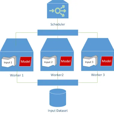
In a distributed setting, a machine learning system is com-prised of a scheduler, a database/file system and a plurality of worker nodes, which are connected through a network. Each worker keeps a partition of the immutable training input and a mutable copy of the machine learning model (Figure 1).

As mentioned in Section I, there are two main platforms for distributed computing: the message passing interface and data-flow frameworks. In Sub-section II-A, we discussed the characteristics of a deep learning application, and now we can discuss how deep learning applications can fit into existing distributed frameworks.

Fig. 1: A distributed machine learning system.

To this end, the MPI framework fits the requirements for scientific applications, since every MPI process has its own local copy of the memory (as illustrated in Figure 2a) and communication is reduced to minimal via messages. How-ever, programmers are responsible for memory management and there is no native support for data beyond the memory capacity.

2) Data-flow & Big Data: A typical big data analytic application takes a large dataset as input and feeds it into a data processing pipeline, after which the data is reduced into a small output.

To this end, the data-flow paradigm suits big data analytic applications. Since it is time costly to move large amounts of data across the network, the compute function is instead sent to the worker. The pair of a compute function and a small chunk of the input data forms a task, which transforms the input data into intermediate data and saves it on the disk; this solves the problem of not having enough main memory to hold the data. The intermediate data is passed onto the next stage for further processing until it is reduced into the final output, and each stage of the data processing pipeline is executed in a lock-step. The workers do not have persistent memory across different tasks or stages. This is illustrated in Figure 2b.

3) Distributed Framework for Machine Learning: Neither MPI or data-flow fits the characteristics of machine learning, as the MPI requires explicit memory management from the users, and the data-flow frameworks suffer from significant overhead costs in task running (discussed further in Section II-D).

Parameter servers [1] are a different approach to the memory persistence and the fault-tolerance problem, which is employed in the TensorFlow [2] library. It works by keeping mutable variables in a remote server, away from error-prone workers. It is not an ideal solution since the variables are not local to the workers, and this adds extra latency and traffic to the network. It is not the best approach going forward for larger

(a) MPI Processes (b) Analytic Tasks

Fig. 2: A comparison between MPI processes and analytic tasks.

scale and more advanced high performance compute clusters. There are two solutions: (i) adapt the data-flow frameworks for machine learning; (ii) add distributed memory management support for MPI. Adapting the data-flow frameworks is a better choice, since data-flow frameworks are data-oriented and traditionally used for data analytics and machine learning, and more and more analytic workloads are migrating to high performance clusters.

C. Survey of data analytics frameworks

Modern data analytics frameworks arose from the MapRe-duce[3] paradigm for batch processing large amounts of data, which is a simple fixed data processing pipeline consisting of a Map and a Reduce stage, leading to a different approach of ‘moving compute to data’. After MapReduce, there has been research on improving the flexibility of the pipeline, and as a result, Directed-Acyclic-Graph (DAG) and Timely-Graph have been adopted in Dryad [4] and Naiad [5] respectively. Apache Spark is the mainstream data-flow framework, which is consideredMapReduce2.0. The core of the Spark framework is the DAG engine for scheduling and the Resilient Distributed Dataset (RDD) [6] for in-memory analytics.

Data-flow for batch processing does not satisfy various analytical applications, such as stream processing and graph analytics. As a result, there have been new frameworks: (i) Storm [7] and Flink [8] for stream processing; (ii) Pregel [9], GraphLab [10] and PowerGraph [11] for graph analytics. How-ever, the fundamental mechanisms are similar: an application consists of smaller short-term tasks which carry out a function which may or may not produce side-effects on the state of the data.

D. Apache Spark & Resilient Distributed Dataset

fast in-memory computation, which is useful for data to be reused repeatedly. A Spark program is expressed as RDD transformations in a DAG graph, the DAG engine will then generate a physical execution plan, and schedule tasks onto available processors.

The design of RDD and the DAG data-flow engine is inefficient for deep learning and machine learning in general, for a number of reasons in regard to the memory management and data-flow model.

In regard to the Resilient Distributed Dataset (RDD), firstly, it is immutable, meaning changes to the contents are done through transformations that generate yet another RDD and require more memory. Secondly, there is no random access to the records of an RDD, because the state of the dataset is undetermined, so the entire RDD must be computed. As a consequence, RDDs are not suitable to hold machine learning models as they are volatile. Access to only a few records in a dataset is inefficient as it causes the entire dataset and the dependent datasets to be computed. We have made substantial improvements in accordance to the problems mentioned above in our previous work [12], which is also briefly described in Sub-section III-A.

In regard to the data-flow model, there is a barrier between stages in a data-flow pipeline, as such overlapping two de-pendent stages in the same pipeline is not possible (but it is possible to overlap two stages that are not dependent).

Fundamentally, workers in a data-flow framework carry out ‘tasks’, which is a type of short-term process that executes a ‘closure’. As opposed to a normal process that runs throughout the life-span of the program, a data-flow program consists of small tasks that can generate no side-effect outside of the ‘closure’ function. In other words, the workers have no persistent memory. However, it is a common practice to workaround this problem by attaching data to a long running process, and by doing so generates side-effects outside of the closure function, which is not what it was designed to do.

Communication between stages of a data-flow pipeline is through a process called ‘shuffle’, which is not explicitly directed. The sending task saves the shuffle data on the disk and informs the driver process; the receiving task then inquires about the location of the shuffle data from the driver process. Since the task allocation is not pre-determined, it can be anywhere in the cluster, so it is not possible to eagerly transmit data (it is technically capable, but incorrect prediction of the destination incurs a performance penalty).

Finally, there is limited forms of data-flow communication patterns. For example, an ‘all-reduce’ operation can only be expressed as ‘reduce-broadcast’ in a data-flow, which can be inefficient for collective communications. We have also improved Spark communication for the ‘reduce-broadcast’ pattern in our previous work [13], which is described in Sub-section III-B.

E. Improving MapReduce & Spark

From MapReduce to Spark, the shuffle performance has been the main subject of research, which is the data exchange

Algorithm 1 Standard Batch SGD

1: w←parameters of the objectivef unction

2: η←learning rate 3: procedure SGD(w,η) 4: repeat

5: Randomly select examples. 6: Compute gradient5Q(w).

7: Update parameters w with learning rate η, w = w−η5Q(w).

8: untilminimum is reached 9: end procedure

between two stages in a data pipeline. For MapReduce, research mainly focuses on overlapping the Map andReduce stages, by eagerly sending the intermediate Map results to the reducer task, as seen in [14] & [15]. For Spark, there have been attempts to utilize hardware advancements such as Remote-Direct-Memory-Access (RDMA) to improve shuffle performance as seen in [16] & [17].

F. Stochastic Gradient Descent

For machine learning algorithms in general (not just neural networks), error is defined as the difference between the predicted value and the actual value, calculated by a ‘loss function’, which is in turn a function of the parameters of the machine learning model. An objective function can be a loss function, with the aim to minimize the error or the value of the loss function by changing the parameters of the model. This is achieved through an optimization algorithm.

Stochastic Gradient Descent (SGD) is an optimization method that has been proven effective in many machine learning applications. SGD is in favour for large datasets, over the original Gradient Descent method, because it approximates the gradient of the loss function (i.e. the derivative of the loss function with respect to the parameters) by using small batches of samples from the dataset, rather than the entire sample population in the original gradient descent method, which is more effective. The SGD optimizes objective functions that are in the form of summations (as shown in Equation 1, whereQ

is the objective function with parameterw, andQiis the value

of the objective function evaluated at the ith observation). Algorithm 1 shows the standard batch SGD algorithm. In each iteration, the gradient of the objective function is computed based on a batch of randomly selected examples from the dataset, after which the parameters w is updated with the equation shown in Line 7 of Algorithm 1.

Q(w) = 1 n

n

X

i=1

Qi(w) (1)

(a) RDD (b) MapRDD

Fig. 3: Data Sampling with Regular RDD (left) and MapRDD (right).

that decreases the learning rate monotonically based on the accumulated sum of past gradients to reduce fluctuation. RMSprop [19] is a further variant to the the Adagrad method that incorporates a decay on the accumulated sum of past gradients to address issues with the learning rate dropping too low. Adam [20] is the state-of-art variant to the SGD algorithm that combines both the momentum methods and the adaptive learning rate methods.

G. Asynchronous Stochastic Gradient Descent (SGD)

Due to the cost of synchronization at the end of the training step, the synchronous SGD does not scale with large clusters, therefore research has been attempting to speed up SGD by removing the synchronization. Hogwild [21] is a lock-free SGD method for shared memory architectures. The idea is that several processes update the parameters asynchronously without locking, so that the processes can be a few steps out-of-sync, but can still converge in spite of losses in accuracy. This is later referred to as the Stale-Synchronous-Parallel (SSP) model. The Downpour SGD described in the Distbelief [22] deep learning library is a similar method to the Hogwild algorithm but implemented on parameter servers, where the parameters are stored in remote servers. Tensorflow [2] is the successor to the Distbelief library and it uses a parameter server like architecture. DeepSpark [23] is a realization of the parameter server approach on the Apache Spark framework, where the driver process acts as the parameter server, but it is inferior to the parameter server implementation, since the parameters can only be stored in a single node and this puts more stress on the network bandwidth. SparkNet [24] proposes a naive parallelization scheme for synchronous data-flow frameworks such as Spark, which simply reduces the frequency of synchronization; it is equivalent to using a larger batch size and by doing so sacrifices the rate of convergence in return.

Fig. 4: A task-based all-reduce implementation.

III. METHODS

In this section, we present our solutions for optimizing deep learning on the Apache Spark framework, which include: (i) efficient memory management with MapRDD in Sub-section III-A, (ii) communication optimization using non-blocking task-based all-reduce in Sub-section III-B, and (iii) a novel asynchronous stochastic gradient descent algorithm using non-blocking all-reduce in Sub-section III-C.

A. Memory Optimization

The memory system in Spark is called the Resilient Dis-tributed Dataset (RDD). Since Spark was initially built for batch-processing, the design of RDD is not efficient for machine learning algorithms, as discussed extensively in Sub-section II-D. The computation of RDDs is synchronous and exhaustive, the entire parent dataset must be loaded in memory in order to create a small subset, which is time consuming and memory inefficient. This often uses up the physical memory capacity and causes out-of-memory exceptions.

MapRDD[12] is an extension of the RDD in our previous work. It works by allowing random access to the individual records in the RDD by utilizing the implicit record level relation between the parent and child datasets with the map transformations. It removes the need to compute and store the entire dataset in-memory or on-disk, this reduces the start-up overhead and the memory usage. As shown in our previous work, initial data loading takes a significant amount of time before training starts, and the application is prone to out-of-memory errors.

We compare how the original RDD and the newMapRDD work in Figure 3. Originally, the input data must be fully loaded in the main memory, and a small sample is selected to be consumed by the training process, as shown in Figure 3a. With MapRDD, only the sparsely selected inputs are loaded into a buffer in the main memory, shown in steps 1-3 of Figure 3b. MapRDD adopted a double-buffering strategy, while the contents in one buffer is being used for training, the other is saved in storage and recycled for the next batch, as shown in steps 4 & 5 of Figure 3b.

Algorithm 2 Asynchronous SGD with non-blocking all-reduce method 1 (corresponding to Equation 3)

1: w←parameters of the network

2: procedureMAIN(w)

3: j←count of training steps

4: fori≤numIterationsdo 5: ∆wj ← −η5Q(wj)

6: ALLREDUCE.SUBMIT(∆wj_{, j)}

7: ∆wj−1← ALLREDUCE.GET(j-1) 8: wj+1_=wj_{+ ∆w}j−1

9: j=j+ 1

10: end for 11: end procedure

B. Communication Optimization

As previously discussed (Section II-D thereduce-broadcast method is inefficient as it creates a bandwidth bottleneck at the root process and impedes the speed of training. The training speed can be accelerated by utilizing the fast computer network in a High Performance Computing (HPC) cluster.

In traditional Message Passing Interface (MPI) platforms used by HPC applications, the summation of gradients in the distributed SGD can be implemented by the all-reduce function. However, as discussed in II-B and previous work [13], MPI should not be directly used in Apache Spark.Instead, to enable all-reduce in the alternate task-based frameworks, we proposed an adapted non-blocking all-reduce implementation [13]. An all-reduce manager was designed, which runs along-side the executor process asynchronously and performs the all-reduce operation on behalf of the tasks. Subsequent tasks can then retrieve the combined values in a later stage, as illustrated in Figure 4. In this way, the all-reduce manager is allowed to use a more efficient all-reduce algorithm instead of the reduce-broadcastdata-flow method, because the underlying algorithm is not exposed to the users. We implemented the butterfly all-reduce algorithm and demonstrated significant speedup with respect to the original reduce-broadcast method (please see [13] for details). Previously, the all-reduce performance was tested in isolation and we studied its impact on the communication cost, but we did not look at how it impacts the overall convergence of the machine learning training. In this work, we apply it with the MapRDD (described in Sub-section III-A) to neural network training in the real-world in a realistic setting.

C. Asynchronous SGD with non-blocking all-reduce

Even with the communication optimized in Sub-section III-B, machine learning on Spark still suffers from the over-head in synchronization, in which the time spent for each training step depends on the slowest worker. Major studies [2] [21] favour a Stale Synchronous Parallel (SSP) scheme for Stochastic Gradient Descent, which offers a trade-off between the training speed and the rate of convergence, relying on a shared memory or a parameter server architecture.

Algorithm 3 Asynchronous SGD with non-blocking all-reduce method 2 (corresponding to Equation 4)

1: w←parameters of the network

2: procedure MAIN(w)

3: j←count of training steps

4: fori≤numIterationsdo 5: ∆wj,local← −η5Q(wj,local) 6: wj ←ALLREDUCE.GET(j) 7: wj+1=wj+ ∆wj−1

8: ALLREDUCE.SUBMIT(wj+1_{, j+1)} 9: j=j+ 1

10: end for 11: end procedure

Due to the synchronous data-flow design, asynchronous machine learning is not possible on Apache Spark, but a naive parallelization scheme has been used in SparkNet, to reduce the overhead in synchronization by a less frequent global summation after a certain number of batches. With the non-blocking all-reduce described in III-B, this opens up possibilities for asynchronous machine learning on Spark.

We modify the original update rule for synchronous stochas-tic gradient descent shown in Equation 2, and we propose two possible alternatives with non-blocking all-reduce, as shown in Equations 3 & 4. The symbols of the equations have the same meanings, where Q(w) is the objective function to be minimized with parameter w, symbol η is the learning rate, subscripti denotes the number of example, and superscriptj

denotes the number of iteration.

For method 1, gradients are calculated based on the weights from the previous iteration (denoted by the term5Qi(wj−1)

in Equation 3), and applied on the weights of the current iteration. For method 2, the weights and gradients are current to the current iteration, but the gradients are generated from the local/non-synchronized version of the weight (denoted by the termQi(wj,local)in Equation 4).

wj+1=wj−η

n

X

i=1

5Qi(wj)/n (2)

wj+1=wj−η

n

X

i=1

5Qi(wj−1)/n (3)

wj+1=wj−η

n

X

i=1

5Qi(wj,local)/n (4)

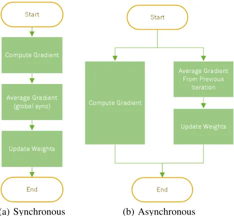
(a) Synchronous (b) Asynchronous

Fig. 5: Comparison of the synchronous and asynchronous SGD methods.

Line 6 and updated with the local gradient in Line 7, which is lastly submitted for all-reduce in Line 8.

1) Theoretical Speedup: The differences between the syn-chronous method and the asynsyn-chronous method are illustrated in Figure 5. For the synchronous method (Figure 5a), the computation of gradient, the global weight aggregation and the weight update occur in a sequential fashion. For the asynchronous method (Figure 5b), the global weight aggre-gation and the weight update are overlapped with the gradient computation, which can potentially accelerate the training speed. However, the asynchronous method trades the rate of convergence for training speed, which may or may not result in an overall improvement. Therefore, an experiment is setup to test the rate of convergence of this method (please see Sub-section IV-C).

Assuming the rate of convergence is comparable and the settings (e.g., learning rate, batch size, number of workers, etc.) are identical, this method provides a maximum speedup of 2x (as shown in Equations 5 & 6), in the ideal case where the computation of the gradient is totally overlapped with the global synchronization of parameters (i.e.Tcompute=Tcomm

in Equation 5).

Speedup= Tcompute+Tcomm max(Tcompute, Tcomm)

(5)

lim

Tcomp→Tcomm

Speedup= Tcomp+Tcomm max(Tcomp, Tcomm)

= 2 (6)

This, in turn, depends on: (I) The neural network model, the processor speed and the batch size, which can have an effect on the computation time; (II) The cluster size, the parameter size and the network speed, which can have an effect on the communication time.

IV. RESULTS

A. Experimental Setup

To evaluate our methods, a real-world neural network deployment was tested on a high-performance cluster, the specification of which is detailed in Table I. The data to be classified is the ImageNet (ILSVRC2012) dataset [25], which contains 1.2 million images of 1000 classes, but only 10% (100 classes) of which was used in our tests. The Caffe-GoogLeNet [26] model was used for training, which is a modified GoogLeNet [27] model for the Caffe library [28], and it has a reported top-1 accuracy of 68.7% on classifying the ILSVRC2012 dataset.

TABLE I: Hardware & Software Specification of the Test Cluster.

Component Detail

Nodes 1 Driver Node, 32 Executor Nodes Cores per Node 20

CPU Intel(R) Xeon(R) CPU E5-2660 v3 @ 2.60GHz Memory 64GB

Harddisk Locally Attached (HDD & SSD)

Interconnect Mellanox Technologies MT26428 (via IPoIB) Software Centos/Linux-2.6, Hadoop 2.7, Spark-2.1.1

TABLE II: Speedup of Neural Network Training of the new method (MapRDD+AllReduce) with respect to the original implementation.

Cluster Size CPU Speedup GPU Speedup_(Expected)

4 2.0 11.2

16 2.3 9.6

32 2.6 9.7

B. Experiment 1: Original vs. MapRDD/All-Reduce

In the first experiment, we compare the original Spark implementation and the modified MapRDD/All-Reduce imple-mentation. We train the first 100 classes of the ILSVRC2012 dataset with a constant batch size of 64 and a varying cluster size (i.e., 4-node, 16-node and 32-node). The candidates in the experiment are algorithmically equivalent, all configurations are the same except for the underlying implementations. We expect changes in the amount of overhead (i.e., startup, scheduling and communication) and the memory usage.

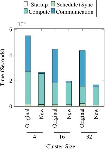
Figure 7 reports the breakdown of costs in training the GoogLeNet model to a 20% accuracy. There is a significant reduction in the communication costs, while the other costs (i.e., startup, compute, scheduling and synchronization) remain comparable. The improvements in the execution time are mainly contributed by the employment of all-reduce described in Sub-section III-B. This is also reflected in the compute-ratio in Figure 6a, which is defined as the proportion of actual computation cost in the total cost; a rise from 31-47% to 82-91% in the compute ratio is observed in our tests.

4 16 32

40 60 80 100

Cluster Size

Compute

Ratio

(%)

Original New

(a) Compute Ratio

4 16 32

0.5 1 1.5

·104

Cluster Size

Memory

Usage

(MB)

Original New

(b) Memory Usage

Fig. 6: A comparison between the original (Spark/RDD) and new (MapRDD/all-reduce) implementations for training the GoogLeNet model on the ImageNet dataset.

Original

Ne

w

Original

Ne

w

Original

Ne

w

0 2 4 6 ·10

4

4 16 32

Cluster Size

T

ime

(Seconds)

Startup Schedule+Sync Compute Communication

Fig. 7: Breakdown of costs to reach 20% accuracy of GoogLeNet with 10% of the ImageNet dataset. Original: Spark & RDD implementation. New: MapRDD & all-reduce implementation.

subset of the original dataset was used and the processing time dominates. We expect a more notable impact with larger input and the use of accelerator cards. However, the improvements are still reflected in the amount of memory used in Figure 6b. A 80% reduction in the memory usage is observed in the

4-node setting where the memory pressure is highest in our test, and subsequently, a 67% and 54% reduction is observed for 16-node and 32-node settings respectively. The advantage of the MapRDD would be more prominent if the full dataset is used, since only 10% of the dataset was used in our tests. Since the MapRDD only keeps the latest batch of samples in memory, the amount of memory used for storing the input data is invariant, the fluctuations in the memory usage for the MapRDD method reflect only the working memory.

Overall, a 2.0x-2.6x speedup is observed in our experiment (listed in Table II), which increases as the cluster size in-creases. We expect little speed gain to be further extracted from this cluster computer since the compute ratio has reach 82-91% as aforementioned. However, since the speedup is mainly contributed by the improvements in communication, a greater speedup is expected if the execution time is com-munication dominant, which is the case for heterogeneous clusters with accelerator cards (such as Graphical Processing Units, GPUs). We tested GoogLeNet with a single GPU chip on a NVidia K80 graphics card using the Caffe & cuDNN library, and the average processing time for a batch size of 64 is 210ms. Assuming a processing time of 210ms per iteration, a speedup between 9.6x-11.2x is to be expected for the same tests carried out by substituting forTcompute andTcompute0 in

Equation 7 (also listed in Table II).

Speedupsync=

Tstartup+Tcompute+Tcomm+Tsync

Tstartup0 +Tcompute0 +Tcomm0 +Tsync0

(7)

C. Experiment 2: Convergence Rate of the Asynchronous Method

0 10 20 30 40 0

1,000 2,000

Top-1 Accuracy (%)

Number

of

iterations

Sync Async

(a) Batch Size 64

0 10 20 30 40

0 500 1,000 1,500

Top-1 Accuracy (%)

Number

of

iterations

Sync Async

(b) Batch Size 128

0 10 20 30 40

0 5 10

Top-1 Accuracy (%)

W

all

clock

time

(hours)

Sync Async

(c) Batch Size 64

0 10 20 30 40

0 5 10 15 20

Top-1 Accuracy (%)

W

all

clock

time

(hours)

Sync Async

(d) Batch Size 128

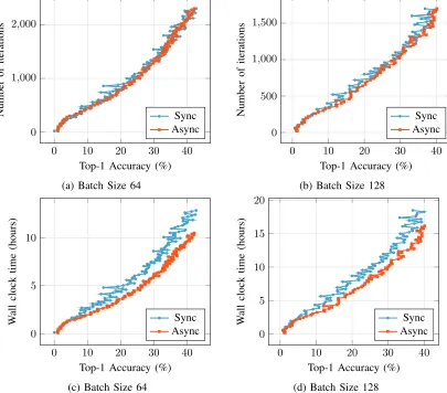
Fig. 8: Top-1 accuracy against the number of iterations/time for training GoogLeNet on the ImageNet dataset.

TABLE III: A comparison of breakdown costs per iteration for the synchronous and asynchronous method (with MapRDD & all-reduce).

Method Batch Size

Compute per iteration

(sec.)

All-reduce per iteration (blocked, sec.)

Sync per iteration (blocked, sec.)

Iterations Accuracy (%) Duration_(sec.)

Sync 64 16.1 2.4 1.6 2200 40 44220

Async 64 16.4 0.0 0.0 2200 40 36080

Sync 128 32.6 2.4 4.2 1700 40 66504

Async 128 34.2 0.0 0.0 1700 40 58140

III-C. As discussed before, this method provides a maximum further speedup of 2x if the compute-to-communication ratio is 1, providing the rate of convergence does not deteriorate faster than the acceleration of the training speed. The compute-to-communication ratio can be manipulated through changing the batch size, the cluster size, the neural network model, etc. But it is based on the assumption that the convergence rate stays the same.

In this experiment, we investigate the rate of convergence of the new asynchronous methods (i.e., Algorithms 2 & 3) with 32 compute nodes and various batch sizes. As the processing power of the accelerators grows, the execution

time will become more communication dominant. The most likely solution to gain speedup is by increasing the size of the batch for each training iteration, to bring the compute-to-communication ratio closer to 1. But it is important to understand how the rate of convergence react to the changes in the batch size.

We tested both Algorithm 2 & 3. Unfortunately, Algorithm 2 failed after a few iterations as the error became too great. Therefore, only the results of Algorithm 3 will be shown in the rest of this section.

8b.

By comparing the same batch size, the accuracy with respect to the number of iterations, for the synchronous method and the asynchronous method, overlap on top of each other. It is also observed that the accuracy for the asynchronous method grows more steadily, whilst the accuracy for the synchronous method fluctuates.

By comparing different batch sizes, it is observed that the rate of convergence for larger batch size with respect to the number of training steps increases. In the case of accelerated clusters, this implies that faster convergence can be obtained by increases the batch size without additional wall clock time, since more computation can be overlapped with the communication. This can potentially provide more than 2x speedup (the maximum speedup derived from Equation 6 in Sub-section III-C) to reach the same accuracy with respect to the synchronous method.

With respect to wall clock time, the asynchronous method provide a 1.0-1.2x speedup over the synchronous method with the same batch size on a homogeneous cluster, as shown in Figures 8c & 8d. This is contributed by the overlapped between the computation and the communication. As shown in Table III, the blocked all-reduce and synchronization costs for asynchronous method are reduced to zero, in return for a slight increase in the compute time. The increase in compute time is caused by the shared workload of the neural network training and all-reduce, which is not expected in a heterogeneous cluster with accelerator cards where the training is performed by the accelerator card and the all-reduce is performed by the CPU processors.

The amount of actual speedup is also dependent on the compute-to-communication ratio, as well as the convergence rate, as explained earlier in Sub-section III-C. For a homo-geneous cluster, the execution time is computation dominant, however, for an accelerated compute cluster, it switches from compute dominant to communication dominant. For example, the compute-to-communication overhead for a batch size of 64 with our experiment setup is around 4, but it drops to 0.05 if an NVidia K80 graphics card is used (assuming a single gpu is used and the processing time is approximately 0.2 seconds). This means a batch size of 20x64 is needed for a compute-to-communication ratio of 1, which can be achieved by 20 mini-batches in a single step. It is a question of whether the convergence rate stays the same with a large sample batch (20x64). The other solution is to accelerate the communication further with Remote Direct Memory Access (RDMA) as it was applied on the Spark shuffle module in [16] & [17]. The current implementation relies on the IPoIB interface that must perform extra data copies by the processors, which causes processor contention between the computation and data copying and leads to a higher latency.

V. CONCLUSION& FUTUREWORK

In this work, we studied the characteristics of deep learn-ing/machine learning applications and the major distributed computing platforms in the context of machine learning. We

introduce Apache Spark, a data-flow framework, and the challenges for its use in machine learning, in terms of memory management, communication costs and synchronization over-heads.

We proposed solutions to these challenges, which includes: (I) MapRDD for more efficient memory management; (II) A task-based all-reduce implementation for more efficient communications; (III) A new asynchronous stochastic gradient descent algorithm using non-blocking all-reduce for reducing synchronization overheads.

Through experimenting the GoogLeNet neural network model on classifying the ImageNet dataset, it demonstrated: (I) An up to 2.6x overall speedup, or a 11.2x theoretical speedup with NVidia K80 graphics cards on a 32-node cluster; (II) A significant rise in compute ratio from 31-47% to 82-91%; (III) An up to 80% reduction in memory usage, and we expect a higher percentage with the full dataset; (IV) A compara-ble convergence rate with the new asynchronous stochastic gradient descent algorithm with respect to the synchronous method, and faster convergence with a larger batch size; (V) An estimated 2x further speedup or an accumulated speedup of 22.4x for a compute cluster equipped with NVidia K80 graphics cards.

With increasing use of accelerator cards, it is possible to process more samples in a single iteration with no extra penalties in wall clock time, as the computation is overlapped with communication using our asynchronous SGD algorithm. At the same time, the levels of neural network models get deeper and the size of the compute cluster grows larger, it is possible to manipulate the settings to achieve 100% efficiency. We will continue to work on the theoretical proof for the convergence of the new asynchronous SGD method, and we will test our method on deeper neural network models and on accelerated compute clusters.

ACKNOWLEDGMENT

This research is supported by Atos IT Services UK Ltd and by the EPSRC Centre for Doctoral Training in Urban Science and Progress (grant no. EP/L016400/1).

REFERENCES

[1] M. Li, D. G. Andersen, J. W. Park, A. J. Smola, A. Ahmed, V. Josifovski, J. Long, E. J. Shekita, and B.-Y. Su, “Scaling distributed machine learning with the parameter server.” inOSDI, vol. 14, 2014, pp. 583– 598.

[2] M. Abadi, P. Barham, J. Chen, Z. Chen, A. Davis, J. Dean, M. Devin, S. Ghemawat, G. Irving, M. Isard, M. Kudlur, J. Levenberg, R. Monga, S. Moore, D. G. Murray, B. Steiner, P. Tucker, V. Vasudevan, P. Warden, M. Wicke, Y. Yu, and X. Zheng, “Tensorflow: A system for large-scale machine learning,” in Proceedings of the 12th USENIX Conference

on Operating Systems Design and Implementation, ser. OSDI’16.

Berkeley, CA, USA: USENIX Association, 2016, pp. 265–283. [Online]. Available: http://dl.acm.org/citation.cfm?id=3026877.3026899 [3] J. Dean and S. Ghemawat, “Mapreduce: simplified data processing on large clusters,”Communications of the ACM, vol. 51, no. 1, pp. 107–113, 2008.

[4] M. Isard, M. Budiu, Y. Yu, A. Birrell, and D. Fetterly, “Dryad: distributed data-parallel programs from sequential building blocks,” in

ACM SIGOPS operating systems review, vol. 41, no. 3. ACM, 2007,

[5] D. G. Murray, F. McSherry, R. Isaacs, M. Isard, P. Barham, and M. Abadi, “Naiad: a timely dataflow system,” in Proceedings of

the Twenty-Fourth ACM Symposium on Operating Systems Principles.

ACM, 2013, pp. 439–455.

[6] M. Zaharia, M. Chowdhury, T. Das, A. Dave, J. Ma, M. McCauley, M. J. Franklin, S. Shenker, and I. Stoica, “Resilient distributed datasets: A fault-tolerant abstraction for in-memory cluster computing,” in Pro-ceedings of the 9th USENIX conference on Networked Systems Design

and Implementation. USENIX Association, 2012, pp. 2–2.

[7] A. Toshniwal, S. Taneja, A. Shukla, K. Ramasamy, J. M. Patel, S. Kulka-rni, J. Jackson, K. Gade, M. Fu, J. Donhamet al., “Storm@ twitter,”

inProceedings of the 2014 ACM SIGMOD international conference on

Management of data. ACM, 2014, pp. 147–156.

[8] P. Carbone, A. Katsifodimos, S. Ewen, V. Markl, S. Haridi, and K. Tzoumas, “Apache flink: Stream and batch processing in a single engine,”Data Engineering, vol. 38, no. 4, 2015.

[9] G. Malewicz, M. H. Austern, A. J. Bik, J. C. Dehnert, I. Horn, N. Leiser, and G. Czajkowski, “Pregel: a system for large-scale graph processing,”

inProceedings of the 2010 ACM SIGMOD International Conference on

Management of data. ACM, 2010, pp. 135–146.

[10] Y. Low, D. Bickson, J. Gonzalez, C. Guestrin, A. Kyrola, and J. M. Hellerstein, “Distributed graphlab: a framework for machine learning and data mining in the cloud,”Proceedings of the VLDB Endowment, vol. 5, no. 8, pp. 716–727, 2012.

[11] J. E. Gonzalez, Y. Low, H. Gu, D. Bickson, and C. Guestrin, “Pow-ergraph: distributed graph-parallel computation on natural graphs.” in

OSDI, vol. 12, no. 1, 2012, p. 2.

[12] Z. Li and S. Jarvis, “Maprdd: Finer grained resilient distributed dataset for machine learning,” in Proceedings of the 5th ACM SIGMOD

Workshop on Algorithms and Systems for MapReduce and Beyond,

ser. BeyondMR’18. New York, NY, USA: ACM, 2018, pp. 3:1–3:9. [Online]. Available: http://doi.acm.org/10.1145/3206333.3206335 [13] Z. Li, J. Davis, and S. Jarvis, “An efficient task-based

all-reduce for machine learning applications,” in Proceedings of the

Machine Learning on HPC Environments, ser. MLHPC’17. New

York, NY, USA: ACM, 2017, pp. 2:1–2:8. [Online]. Available: http://doi.acm.org/10.1145/3146347.3146350

[14] H. Mohamed and S. Marchand-Maillet, “Mro-mpi: Mapreduce over-lapping using mpi and an optimized data exchange policy,” Parallel

Computing, vol. 39, no. 12, pp. 851–866, 2013.

[15] F. Ahmad, S. Lee, M. Thottethodi, and T. Vijaykumar, “Mapreduce with communication overlap (marco),”Journal of Parallel and Distributed

Computing, vol. 73, no. 5, pp. 608–620, 2013.

[16] H. Li, T. Chen, and W. Xu, “Improving spark performance with zero-copy buffer management and rdma,” in Computer Communications

Workshops (INFOCOM WKSHPS), 2016 IEEE Conference on. IEEE,

2016, pp. 33–38.

[17] H. Daikoku, H. Kawashima, and O. Tatebe, “On exploring efficient shuffle design for in-memory mapreduce,” inProceedings of the 3rd ACM SIGMOD Workshop on Algorithms and Systems for MapReduce

and Beyond. ACM, 2016, p. 6.

[18] J. Duchi, E. Hazan, and Y. Singer, “Adaptive subgradient methods for online learning and stochastic optimization,” Journal of Machine

Learning Research, vol. 12, no. Jul, pp. 2121–2159, 2011.

[19] T. Tieleman and G. Hinton, “Lecture 6.5-rmsprop: Divide the gradient by a running average of its recent magnitude,” COURSERA: Neural

networks for machine learning, vol. 4, no. 2, pp. 26–31, 2012.

[20] D. P. Kingma and J. Ba, “Adam: A method for stochastic optimization,”

arXiv preprint arXiv:1412.6980, 2014.

[21] B. Recht, C. Re, S. Wright, and F. Niu, “Hogwild: A lock-free approach to parallelizing stochastic gradient descent,” in Advances in neural

information processing systems, 2011, pp. 693–701.

[22] J. Dean, G. Corrado, R. Monga, K. Chen, M. Devin, M. Mao, A. Senior, P. Tucker, K. Yang, Q. V. Le et al., “Large scale distributed deep networks,” inAdvances in neural information processing systems, 2012, pp. 1223–1231.

[23] H. Kim, J. Park, J. Jang, and S. Yoon, “Deepspark: A spark-based distributed deep learning framework for commodity clusters,” arXiv

preprint arXiv:1602.08191, 2016.

[24] P. Moritz, R. Nishihara, I. Stoica, and M. I. Jordan, “Sparknet: Training deep networks in spark,”CoRR, vol. abs/1511.06051, 2015.

[25] ImageNet, http://www.image-net.org/challenges/LSVRC/2012/, n.d., [Online; Accessed 01-September-2018].

[26] S. Guadarrama, https://github.com/BVLC/caffe/tree/master/models/bvlc googlenet, n.d., [Online; Accessed 01-September-2018].

[27] C. Szegedy, W. Liu, Y. Jia, P. Sermanet, S. Reed, D. Anguelov, D. Erhan, V. Vanhoucke, and A. Rabinovich, “Going deeper with convolutions,”

in2015 IEEE Conference on Computer Vision and Pattern Recognition

(CVPR), June 2015, pp. 1–9.