Abstract—The effect of iron on the uniformity of the field
produced by an axisymmetric thick solenoid is considered. Here two solution to the vector potential and hence the magnetic field components will be derived. The first solution is obtained using a Power series and the other is obtained using the Euler-Maclaurin summation formula, thus converting the doubly infinite summation into an integral. Numerical results for the vector potential and the field components are given as well plots of the field distribution.
Index Terms— Time independent field, Power series, the
Euler-Maclaurin Summation formula
I. INTRODUCTION
n this paper magnetostatic field calculations associated with an axisymmetric conductor of rectangular cross section situated equidistant from two semi-infinite regions of iron of finite permeability are computed. The magnetostatic field associated with iron-free axisymmetric systems has been considered by Boom and Livingstone [2], Garrett [3] and many others. Caldwell [4], Caldwell and Zisserman [5] and [6] have carried out work which takes account of the effects of the presence of iron on such systems. The main advantages of introducing iron are: i. Higher fields are provided for the same current, producing substantial power savings over conventional conductors.
ii. The field uniformity is improved even for superconducting solenoids by placing the iron in a suitable position.
The geometry considered is shown in figure 1, a toroidal conductor V’ of rectangular cross section having inner radius A, outer radius B and length L-2, is located equidistant between two semi-infinite regions of iron of finite permeability a distance L apart, the axis of the torus being perpendicular to the iron boundaries. The region V between the conductor and the iron is assumed insulating. Cylindrical polar coordinates (r,,z) are used where r and z are normalized in terms of L.
Prior to Caldwell [3] the presence of iron in axisymmetric systems had been largely ignored see Loney
Manuscript received August 13 2013.
V.Pavlika is with SOAS, University of London, UK
[8] and Garrett [3] et al. In cylindrical polar coordinates Maxwell’s equations give:
B
0
'
in V
Ce in V
where e is a unit vector in the direction of increasing and C is a constant with
.
B
0
in V and V’ (1)Equation (1) suggests the introduction of a potential A such that
B
A
, axial symmetry impliesr
A
B
z
;(
)
1
0;
zrA
B
B
r
r
So that Maxwell’s equation gives:0
(
)
'
in V
B
A
Ce in V
thus
1
0
1 (
)
0
r z
e
e
e
r
r
z
A
rA
z
r
r
=
0
'
in V
Ce in V
2 1
0
'
in V
A
Ce in V
where
2 2
2
1 2 2 2
1
1
r
r r
r
z
with boundary conditions
0
A
on r = 00
A
asr
0
A
z
on z=0 and z=1Comparison of Magnetostatic Field Calculations
Associated with Thick Solenoids in the
Presence of Iron using a Power Series Approach
and the Euler-Maclaurin Summation Formula
Vasos Pavlika
I
Using the integral representation of the vector potential this gives '
( )
( )
'
|
' |
Vj r
A r
dv
r
r
, hence for finite ,In cylindrical coordinates
2 / 1 2 2 2
)
cos
2
)
'
((
|
'
|
r
r
z
z
r
x
xr
Which can be substituted below in:
'
|
'
|
cos
4
)
,
(
2 0 1 | |0
dxd
dz
r
r
x
K
j
z
r
A
b a nn
(2)With 1
1
K
, known as the image factor.
Noting that
A r z
( , )
is an odd function in r and an even function in z thenA
can be expanded as a power series about the z axis giving:
n m m m nz
I
r
K
z
r
A
0 1 2 | |0
(
)
)
,
(
(3)
where expression (2) gives
n m m m nz
I
r
K
z
r
A
0 1 2 | |0
(
)
)
,
(
And
10
[[
log
|
|]
]
4
1
)
(
z
w
ex
ba zI
with w=z’-z-n and 2 = x2+w2. Substituting expression (3) into expression (2) gives
2
| | 2 1 2 1
2
1 1
( )
4 (
1)
( )
0
n m m m
m
n m m
I z
K
m m
r
I z
r
z
equating coefficients of Im(z)
,....
2
,
1
,
0
,
0
)
(
)
(
)
1
(
212
m
z
z
I
z
I
m
m
m m So that)!
1
(
!
2
)
(
)
1
(
)
(
2 2 0
m
m
z
I
z
I
m m m m and
n m m m m m nr
m
m
z
I
K
z
r
A
0 1 2 2 2 0 | | 0)!
1
(
!
2
)
(
)
1
(
)
,
(
To relate this to the work of Garrett [3] let
1
1
( , )
log |
|
0[[ ( , )] ]
14
b
e a z
j
a x w
w
x
I
a x w
1
( )
2
A z
where 1
( , )
[[ log |
|] ]
12
b a z
j
a x w
w
x
(4)and
1
[[
( , )] ]
2
b m m a z
j
A
a
x w
(5) so that
n m m m m m nm
m
r
z
A
m
K
z
r
A
0 1 2 1 2 1 2 | | 0)!
1
(
!
2
)
(
)!
2
(
)
1
(
)
,
(
n m m m m nm
r
z
A
m
K
0 1 2 1 2 | | 0!
)!
2
2
(
)
(
!
)!
1
2
(
)
1
(
where (2m-1)!!= 1.3.5…(2m-1), and (2m+2)!!= 2.4.6…(2m+2), with
)
(
1
1 1a
z
m
A
m m m
(6)
so for the field components
n m m m m n zm
r
z
A
m
K
z
r
B
0 1 2 1 2 | | 0!
)!
2
(
)
(
!
)!
1
2
(
)
1
(
)
,
(
and
n m m m m n r m r z A m K z r B 0 1 2 2 2 | | 0 ! )! 2 2 ( ) ( ! )! 1 2 ( ) 1 ( ) , ( Hence
n nA
r
A
r
A
r
K
z
r
A
....)
16
8
2
(
)
,
(
5 5 3 3 1 | | 0
n n zA
r
A
r
A
K
z
r
B
....)
8
3
2
(
)
,
(
5 4 3 2 1 | | 0
and
n n rA
r
A
r
A
r
K
z
r
B
...)
16
5
8
3
2
(
)
,
(
6 5 4 3 2 | | 0
The first five terms will be quoted, the remainder can be obtained from the recurrence relations equations (4), (5) and (6). So that
2 2 1/ 2 1
2
[[
2 2 1/ 2log (
(
)
)] ]
2 (
)
b
e a z
j
x
A
x
w
x
w
x
13
[[
2 2 1/ 2 2 2 3/ 2] ]
2 (
)
(
)
b a z
j
x
xw
A
w
x
w
x
4 2 2 3/ 2 2 2 5 / 2
1 2 2 3/ 2
3
[[
12 (
)
(
)
] ]
(
)
b a z
j
x
xw
A
w
x
w
x
xw
w
x
5 2 2 5 / 2 2 2 3/ 2
3
2 2 7 / 2 2 2 3/ 2
2 1 2 2 5 / 2
3
6
[[
48 (
)
(
)
15
(
)
(
)
3
] ]
(
)
b a z
j
xw
xw
A
w
x
w
x
xw
x
w
x
w
x
xw
w
x
and6 2 2 5 / 2 2 2 3/ 2
2 3
2 2 7 / 2 2 2 7 / 2
4 1
9
9
[[
240 (
)
(
)
15
(
)
(
)
] ]
ba zj
x
xw
A
w
x
w
x
xw
xw
w
x
w
x
xw
II. CALCULATION OF THE FIELD COMPONENTS USING THE EULER-MACLAURIN SUMMATION FORMULA
Here use of the Euler-Maclaurin summation will be used to convert the doubly infinite sum corresponding to the image coils to an integral. Much literature exists on the derivation of the formula thus only the final formula will be quoted. We have the vector potential given by expression (2), so that considering the summation and defining:
| | 2 2 1/2
((
)
)
n
n
K
S
n
Where
2 2 2
cos ,
2
cos
'
x
r
x
xr
and
z
z
so that
| | | |
2 2 1/2 2 2 1/2 2 2 1/2
0
((
)
)
0((
)
)
(
)
n n
n n
K
K
S
n
n
which may be written as
1 2 2 2 1/2
0 0
( )
( )
,
(
)
n n
S
f n
f n
say
2 2 1/2 0
( )
(
)
n
f n
where
f n
( )
f n
1( )
f n
2( )
. So that the effect of theimage coils has been separated from the main coil. To these images we apply the Euler-Maclaurin Summation formula. Considering the term
0 1 1 1
0
1
(
0
)
(
)
2
1
)
(
)
(
n
f
n
dn
f
f
f
n
+
[
(
0
)
(
)]
...
720
1
)
0
(
)
(
12
1
'''1 ''
' 1 '
1 '
1
f
f
f
f
Letting
0 1 0 2 2 1/2
1
)
)
((
)
(
)
(
dn
n
k
dn
n
f
I
n
0
((
n
)
2 2)
1/2dn
e
n
Where
log
|
1
|
K
e
and,
1
1
1
K
So clearly the method will not cater for the case when
1
, but this is expected as that is the iron free situation. In order to make any progress with this integral the integrand will be expanded in a Maclaurin series in
which will be a small parameter. Thus)
(
)
0
(
!
2
)
0
(
)
0
(
)
(
1'' 32 '
1 1
1
I
I
I
O
I
.So that
(
)
(
)
(
)
2
)
(
)
0
(
0 0
0
0 2 2 1/2
1
N
E
S
dn
n
e
I
n
Where
S
(
z
)
Schlafli’s polynomial of order
,S
0(
z
)
0
z
, Watson [11].
)
(
z
E
Weber’s function of order , Watson [11] and
)
(
z
N
Neumann’s function of order , Watson [11 ]. So that
)
(
|
)
)
((
)
(
)
(
)
(
2
)
0
(
2 0
0 2 2 1/2
0 0
0 1
O
dn
n
e
N
E
S
I
n
now
dn
n
ne
I
n
0 2 2 3/2
' 0
)
(
)
0
(
)
(
)
(
)
(
)
(
)
(
2
)
(
2
0 2 2 3/2
0 0
0 1
O
dn
n
ne
N
E
S
I
n
Furthermore
2 / 1 2 2 1
)
(
)
0
(
f
andf
1(
)
0
2 / 3 2 2
2 2
' 1
)
(
)
(
.
)
0
(
f
andf
1'(
)
0
So that
).
(
)
(
12
)
(
.
2
1
)
(
)
(
)
(
)
(
2
)
(
2 2
/ 3 2 2
2 2
2 / 1 2 2
0 2 2 3/2
0 0
0 0
1
O
dn
n
ne
N
E
S
n
f
n n
Now considering
0 2 2 2
0
2
(
0
)
(
)
2
1
)
(
)
(
n
f
n
dn
f
f
f
n
[
(
0
)
(
)]
...
720
1
)
0
(
)
(
12
1
'''2 '' ' 2 ' 2 '
2
f
f
f
f
With similar manipulation as just performed it can be shown that
).
(
)
(
12
)
(
.
2
1
)
(
)
(
)
(
)
(
2
)
(
2 2 / 3 2 2 2 2 2 / 1 2 20 2 2 3/2
0 0 0 0 2
O
dn
n
ne
N
E
S
n
f
n n
So that
).
(
)
(
.
6
1
)
(
)
(
)
(
2
2 2 / 1 2 2 0 0 0
O
N
E
S
S
To proceed with this method these special functions must be written in a form so that they can be integrated over the volume of interest.
III. NEUMANN’S FUNCTION,BESSEL FUNCTION OF THE SECOND KIND
Here the Bessel function of the second kind has been obtained, taking the definition of the Neumann function as
sin
)
(
)
(
cos
)
(
x
J
x
J
x
N
Evaluating
N
n(x
)
by l’Hopital’s rule for indeterminant forms (i.e. for
n
(integer))gives
n n
n
x
J
x
J
x
N
(
)
(
1
)
(
)
|
1
)
(
With n m m m nx
m
n
m
x
J
2 02
.
)
1
(
!
)
1
(
)
(
i.e. The usual Bessel function of the first kind of order n. Using
)
(
log
)
(
x
x
x
d
d
e
and)))
(
(
(log
))
(
(
z
dz
d
z
dz
d
e
giving r n n r r n r r e n nx
r
r
n
r
n
F
r
F
x
r
n
r
x
x
J
x
N
2 1 0 2 02
.
!
)!
1
(
1
))
(
)
(
(
2
.
)!
(
!
)
1
(
1
)
2
(
log
)
(
2
)
(
Where F(r) and F(n+r) are the digamma functions (Abramowitz and Stegun [1]) arising from the differentiation of the gamma function when expressed as an infinite limit. Using properties of the digamma function gives: r n n r r p r n r r n n p e n
x
r
r
n
n
p
p
x
r
n
r
x
J
p
x
x
N
2 1 0 1 2 0 12
.
!
)!
1
(
1
1
1
2
.
)!
(
!
)
1
(
1
)
(
1
2
1
'
)
2
(
log
2
)
(
Where
'
is the Euler-Mascheroni constant (Abramowitz and Stegun [1]). So finally for n=0 the limiting value is:
log
(
)
'
log
(
2
)
(
)
2
)
(
20
x
x
O
x
N
e
e
.IV. THE WEBER FUNCTION AND ITS RELATION TO THE STRUVE FUNCTION
By definition the Weber function may be expressed as
0sin(
sin
)
1
)
(
x
z
d
E
The relationship between Weber’s function and the Struve function is, for n being a positive integer or zero (Abramowitz and Stegun [1])
( 1)/20 1 2
)
(
)
2
1
(
2
1
)
2
1
(
1
)
(
n k n k nz
H
k
n
z
k
x
E
Where
H
n(
z
)
is the Struve function defined by
0 2 2 12
1
)
2
3
(
)
2
3
(
)
1
(
)
2
1
(
)
(
k k k kk
k
z
x
H
It follows that
...)
5
3
1
3
1
(
2
)
(
)
(
)
(
2 2 2
5
2 2
3 0
0 0
z
z
z
z
E
z
H
z
E
This gives
).
(
)
(
.
6
1
))
2
(
log
'
)
(
log
2
2
2 2
/ 1 2
2
O
S
e e
where to avoid confusion the Euler-Mascheroni constant has been denoted by
'
and
x
cos
. Thus integration over the volume of interest can now be performed. That is
).
(
'
}
)
(
.
6
1
))
2
(
log
'
)
(
log
2
2
{
4
)
,
(
2 2
/ 1 2 2
2 0
1 0
O
dz
dxd
j
z
r
A
ba
e e
V. CONSIDERING THE ORDER
TERM IN THE EXPRESSION FORA
(
r
,
z
)
Considering the
O
(
)
term and denoting this as
ba
dxd
dz
j
20 1
2 / 1 2 2
0
'
)
(
24
(7)Performing the
integration first gives
b a
xdxdz
d
j
20 2 1/2
1 0
)
cos
(
cos
'
24
Where
2
(
z
z
'
)
2
x
2
r
2and
2
xr
. Slight manipulation leads to
b a
k
u
du
u
dxdz
x
j
/20 2 2 1/2
2 1
0
)
sin
1
(
1
sin
2
'
24
where
2
2
(
z
z
'
)
2
(
x
r
)
2 and2 2
2
)
(
)
'
(
4
r
x
z
z
xr
k
, with
u
2
2
.
It can be shown that (Gradsteyn and Ryzhik [7])
)
,
,
,
(
)
,
(
2
1
)
sin
1
(
cos
sin
22 /
0 2 2
1 2 1 2
k
F
B
dx
x
k
x
x
Where B(m,n) is the Beta function and
F
(
a
,
b
,
c
,
z
2)
is the Hypergeometric function, so that) , 2 , 2 3 , 2 1 ( ) 2 1 , 2 3 ( )
sin 1 (
1 sin
2 2
2 /
0 2 2 1/2
2
k F
B du u k
u
,
1
,
)
2
1
,
2
1
(
)
2
1
,
2
1
(
2
1
2k
F
B
So that
ba
z
z
x
r
x
B
j
12 / 1 2 2
0
.
)
)
(
)
'
((
)
2
1
,
2
3
(
6
'
)
,
2
,
2
3
,
2
1
(
*
F
k
2dxdz
ba
z
z
x
r
x
B
j
12 / 1 2 2
0
.
)
)
(
)
'
((
)
2
1
,
2
1
(
12
'
)
,
1
,
2
1
,
2
1
(
*
F
k
2dxdz
, (8)with
)
(
)
(
)
(
)
,
(
m
n
n
m
n
m
B
, it can also be shown that2
)
2
1
,
2
3
(
B
and)
2
1
,
2
1
(
B
.Pavlika [10] has shown that the integrals containing the series of the hypergeometric function are uniformly convergent in the interval of integration so that with some algebraic manipulation it can be shown that Pavlika [10]
ba
z
z
x
r
x
j
12 / 1 2 2
0
.
)
)
(
)
'
((
{
12
dxdz
n
k
E
n
n n
}
!
*
0 2
Where
E
n
C
n
D
n and)
,
1
(
)
,
2
1
)(
,
2
3
(
,
)
,
2
(
)
,
2
3
)(
,
2
3
(
n
n
n
D
n
n
n
C
n
n
with0
),
1
)...(
1
(
)
(
)
,
(
)
,
(
k
k
k
k
.VI. CONSIDERING THE ORDER
k
0TERM IN THE EXPRESSION FOR
.Considering the term and denoting this integral as
K
0 that is:
ba
z
z
x
r
dxdz
x
jE
K
12 / 1 2
0 0
0
'
)
(
)
'
((
12
thus
)
(
(
log
)
2
[[(
12
2 2 2
0 0
0
ru
u
u
jE
K
e
2 / 1 2 2
)
(
2
u
n z
n z r b
r a e
u
u
r
2 2 1/2 1]
]
)
(
(
log
Where u = x + r and
z
z
'
.VII. CONSIDERING THE ORDER
k
2 TERM IN THE EXPRESSION FOR
.Considering the
O
(
k
2)
term and denoting this term as2
K
, say where:
ba
z
z
x
r
dxdz
x
r
jE
K
12 / 3 2
3 1
0
2
'
)
(
)
'
((
3
Computing these integrals gives
2 / 1 2 2 1
0
2
[[
(
)
3
r
w
w
u
jE
K
)
)
(
(
log
3
ru
ew
w
2
u
2 1/2
2 / 1 2 2 2
/ 1 2 2
)
(
3
)
)
(
(
log
3
rw
ew
w
u
r
w
u
)
)
(
(
log
3
2 2 2 1/2u
w
w
r
e
12 / 1 2 2 3
]
)]
)
(
zz r b
r a
uw
u
w
r
Where u = x + r and w = z - z’. Therefore
).
(
'
}
)
2
(
log
'
)
(
log
2
2
{
4
)
,
(
2 2
0
2 0
1 0
O
K
K
dz
dxd
j
z
r
A
e e
b a
(9)
VIII. CONSIDERING THE ORDER
0
TERM IN THE EXPRESSION FOR)
,
(
r
z
A
.Considering the
O
(
0)
term in equation (9) and denoting this term by
0 , say where
ba
e
x
dxd
dz
j
20 1 0
0
(
'
log
(
2
))
cos
'
2
0
So that
'
}
ln
2
2
{
4
)
,
(
20 1
0
j
dxd
dz
z
r
A
ba
K
0
K
2
O
(
2).
IX. CONSIDERING THE ORDER
AND
TERMS IN THE EXPRESSION FORA
(
r
,
z
)
.Considering the
O
(
)
andO
(
)
terms and denoting this integral as
ba
x
x
r
xr
j
20
2 / 1 2
2 0
1
(
1
2
)
(
cos
(
2
cos
)
2
x
cos
)
dxd
Where
log
e|
|
. With slight manipulation it can be shown that
ba
x
x
r
dx
j
)
(
)
2
1
(
4
01
/2
0
2 / 1 2 2 2
)
sin
1
(
sin
u
du
u
ba
x
x
r
dx
j
)
(
)
2
1
(
2
0
2 / 0
2 / 1 2 2
)
sin
1
(
u
du
Where
u
xr
r
x
k
k
k
2
2
,
2
,
,
,
1
2
2 2 22 2 2 2 2
It can be shown (see Gradsteyn and Ryzhik [7]) that:
)
,
2
2
,
2
1
,
2
1
(
)
2
1
,
2
1
(
2
1
)
sin
1
(
cos
sin
2 2
/ 0
2 / 1 2 2
k
n
m
m
F
n
m
B
du
u
k
u
u
nm
For
m
1
,
n
1
,
|
k
2|
1
, whereB
(
p
,
q
)
is the Beta function andF
(
a
,
b
,
c
,
z
2)
is the hypergeometric function whose convergence has already been discussed, Proceedings of the International MultiConference of Engineers and Computer Scientists 2014 Vol II,thus
1can easily be evaluated. Now the term containingthe logarithm of
must be considered, denoting this integral as
2 then
ba
xdx
j
)
2
1
(
4
0
2
2
0
2 2
)
cos
2
(
cos
x
r
xr
d
Once again this integral has be computed see Pavlika [10], thus finally
)
(
)
,
(
0 1 1 2
2
r
z
K
K
O
A
Where
K
0,
K
2,
1and
2 are now known. X. CONCLUSIONSThe two methods of solution were found to be in good agreement however more terms are required for the method of solution based on the Euler-Maclaurin summation formula. The summations were performed from -200 to 200 with a change only in the fourth decimal place occurring when the number of terms in the summation was doubled. The effect of the permeability of the iron is shown in figures 2, 3, 4 and 5.
REFERENCES
[1] Abramowitz. M and Stegun, I.A, “Handbook of Mathematical Functions”. Dover Publications, Inc, New York.
[2] Boom, R.W., and Livingstone. R.S, Proc. IRE, 274 (1962).
[3] Garrett, M.W, “Axially symmetric systems for generating and measuring magnetic fields”. J. Appl. Phys., 22, 1091 (1951). [4] Caldwell. J, “Magnetostatic field calculations associated with
superconducting coils in the presence of magnetic material”. IEEE, Transactions on Magnetics, Vol. MAG-18, 2, 397 (1982). [5] Caldwell, J and Zisserman A., “Magnetostatic field calculations in
the presence of iron using a Green’s Function approach”. J.Appl. Phys.D 54, 2, (1983a).
[6] Caldwell, J and Zisserman A, “A Fourier Series approach to magnetostatic field calculations involving magnetic material” accepted for publication in J.Appl. Phys (1983b).
[7] Gradsteyn. I.S and Ryzhik., I.M. “Tables of Integrals Series and Products”, Academic Press (1969).
[8] Loney, S.T, “The Design of Compound Solenoids to Produce Highly Homogeneous Magnetic Fields”. J.Inst. Maths Applics (1966) 2, 111-125.
[9] Pavlika, V, “Vector Field Methods and the Hydrodynamic Design of Annular Ducts”, Ph.D thesis, University of North London, Chapter II, 1995.
[10] Pavlika, V, “Vector Field Methods and the Hydrodynamic Design of Annular Ducts”, Ph.D thesis, University of North London, Chapter III, 1995.
[image:7.595.305.541.49.263.2][11] Watson. G.N, “A treatise on the theory of Bessel functions”. Cambridge University press (1980).
Table 1: Values of
A
(
r
,
z
)
using the Power series. r Z =103 =102 =10 =10 0.1 0 0 0 0
0.1 0.1 0.8958 0.8808 0.7580 0.3496 0.2 0.1 1.7913 1.7614 1.5167 0.7022 0.3 0.1 2.6862 2.6416 2.2767 1.0609 0.4 0.1 3.5802 3.5212 3.0386 1.4287 0.5 0.1 4.4730 4.4000 3.8031 1.8095
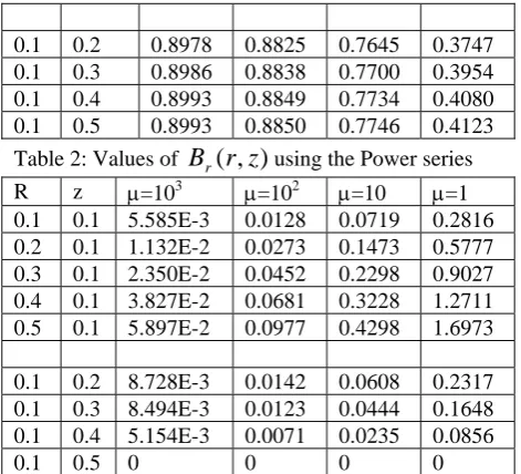
[image:7.595.306.552.468.617.2]0.1 0.2 0.8978 0.8825 0.7645 0.3747 0.1 0.3 0.8986 0.8838 0.7700 0.3954 0.1 0.4 0.8993 0.8849 0.7734 0.4080 0.1 0.5 0.8993 0.8850 0.7746 0.4123 Table 2: Values of
B
r(
r
,
z
)
using the Power series R z =103 =102 =10 =1 0.1 0.1 5.585E-3 0.0128 0.0719 0.2816 0.2 0.1 1.132E-2 0.0273 0.1473 0.5777 0.3 0.1 2.350E-2 0.0452 0.2298 0.9027 0.4 0.1 3.827E-2 0.0681 0.3228 1.2711 0.5 0.1 5.897E-2 0.0977 0.4298 1.6973 0.1 0.2 8.728E-3 0.0142 0.0608 0.2317 0.1 0.3 8.494E-3 0.0123 0.0444 0.1648 0.1 0.4 5.154E-3 0.0071 0.0235 0.0856 [image:7.595.307.562.643.781.2]0.1 0.5 0 0 0 0
Table 3: Values of
B
z(
r
,
z
)
using the Power Series. r Z =103 =102 =10 0.1 17.9170 17.6164 6.9822 0.1 0.1 17.0150 17.6151 7.0023 0.2 0.1 17.9091 17.6112 7.0628 0.3 0.1 17.8991 17.6047 7.1635 0.4 0.1 17.8852 17.5965 7.3046 0.5 0.1 17.8673 17.5839 7.4860 0.1 0.2 17.9732 17.6546 7.5233 0.1 0.3 17.9723 17.6771 7.9259 0.1 0.4 17.9861 17.6996 8.1803 0.1 0.5 17.9867 17.7015 8.2673 Table 4: Values of
A
(
r
,
z
)
using the Power series r Z =103 =102 =10 =10 0.1 0 0 0 0
0.1 0.1 0.89172 0.881238 0.7576 0.3481 0.2 0.1 1.79492 1.762867 1.5141 0.6902 0.3 0.1 2.69390 2.645277 2.2679 1.0201 0.4 0.1 3.59466 3.528858 3.0178 1.3319 0.5 0.1 4.49780 4.414002 3.7625 1.6196 0.1 0.2 0.89782 0.882508 0.7642 0.3733 0.1 0.3 0.89596 0.883737 0.7693 0.3926 0.1 0.4 0.89920 0.884629 0.7726 0.4049 0.1 0.5 0.89943 0.884955 0.7738 0.4091
Table 5: Values of
B
r(
r
,
z
)
using the Power seriesr z =103 =102 =10 =1
0.1 0.1 5.832E-3 0.0163 0.1042 0.0362 0.2 0.1 1.315E-2 0.0343 0.2120 0.0776 0.3 0.1 2.344E-2 0.0556 0.3674 0.1426 0.4 0.1 3.819E-2 0.0820 0.4521 0.1599 0.5 0.1 5.887E-2 0.1151 0.5914 2.0972 0.1 0.2 8.426E-3 0.0166 0.0852 0.2937 0.1 0.3 8.083E-3 0.0136 0.0607 0.2072 0.1 0.4 4.898E-3 0.0071 0.0316 0.0107
0.1 0.5 0 0 0 0
[image:7.595.42.273.691.781.2]Fig. 1. A toroidal conductor V’ of rectangular cross section located midway between two semi infinite regions of iron of finite permeability. The region V is assumed to be insulating.
0.2 0.4 0.6 0.8 1
z
6.5 7.5 8 8.5
Bz
H
r,zL
Fig. 2. The variation of Bz(r,z) with r and z for two
semi-infinite regions of iron of unit permeability. :r=0.3,
:r=0.2, •:r=0.1
0.2 0.4 0.6 0.8 1
z
17.94 17.96 17.98 18.02 18.04
Bz
H
r,zL
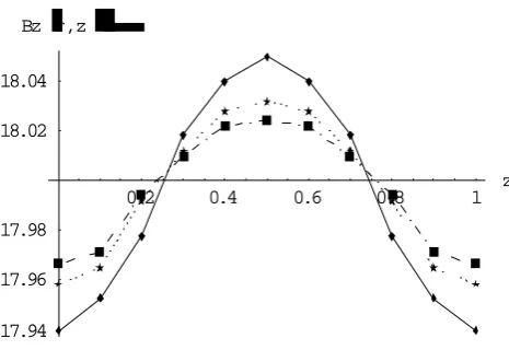
Fig. 3. The variation of Bz(r,z) with r and z for two
semi-infinite regions of iron of semi-infinite permeability. :r=0.1,
:r=0.2, •:r=0.3
0.2 0.4 0.6 0.8 1
z
-1 -0.5 0.5 1
[image:8.595.315.549.265.423.2]Br
H
r,zL
Fig. 4. The variation of Br(r,z) with r and z for two
semi-infinite regions of iron of unit permeability. :r=0.1,
:r=0.2, •:r=0.3
0.2 0.4 0.6 0.8 1
z
-0.04 -0.02 0.02 0.04
Br
H
r,zL
Fig. 5. The variation of Br(r,z) with r and z for two
semi-infinite regions of iron of semi-infinite permeability. :r=0.1,
:r=0.2, •:r=0.3
[image:8.595.48.282.303.458.2] [image:8.595.47.280.516.676.2]