Optimum Mode Switching Assisted Adaptive Modulation

Optimum Mode-Switching Assisted Adaptive Modulation

Byoung-Jo Choi and Lajos Hanzo

1

Dept. of ECS, University of Southampton, SO17 1BJ, UK.

Tel: +44-23-8059-3125, Fax: +44-23-8059-4508

Email:lh

1

@ecs.soton.ac.uk, http://www-mobile.ecs.soton.ac.uk

Abstract – Adaptive modulation techniques combat

fad-ing by employfad-ing a suitable modulation mode dependfad-ing on the instantaneous channel conditions for improving the Bit Error Rate (BER) performance or the average through-put. Based on a generic model of constant-power adaptive modulation, exact closed form expressions of the average BER and the average throughput are derived, when em-ploying square Quadrature Amplitude Modulation (QAM) or Phase Shift Keying (PSK) as the constituent modulation modes, operating over a Nakagami fading channel. The optimum modulation-mode switching levels, achieving the highest possible throughput under the constraint of the av-erage BER, are obtained using the Lagrangian optimisa-tion method. Adaptive modulaoptimisa-tion employing the optimum switching levels shows a superior performance, while main-taining a constant average BER.

1. INTRODUCTION

Mobile communications channels typically exhibit time-variant channel quality fluctuations [1] and hence conventional fixed-mode fixed-modems suffer from bursts of transmission errors, even if the system was designed to provide a high link margin. An efficient approach to mitigating these detrimental effects is to adaptively adjust the transmission format based on the near-instantaneous channel quality perceived by the receiver, which is fed back to the transmitter with the aid of a feedback chan-nel [2]. Hayes [3] proposed transmission power adaptation, while Cavers [4] suggested invoking a variable symbol dura-tion scheme in response to the perceived channel quality at the expense of a variable bandwidth requirement. Since a variable-power scheme increases both the transmitted variable-power require-ments and the level of co-channel interference [5], variable-rate Adaptive Quadrature Amplitude Modulation (AQAM) was proposed by Steele and Webb as an alternative, employing var-ious star-QAM constellations [5, 6]. With the advent of Pi-lot Symbol Assisted Modulation (PSAM), Otsuki, Sampei and Morinaga [7] employed square constellations instead of star constellations for AQAM, as a practical fading counter mea-sure. Analysing the channel capacity of Rayleigh fading chan-nels [8, 9], Goldsmith and Varaiya showed that variable-power, variable-rate adaptive schemes are optimum in terms of ap-proaching the channel capacity and they characterised the

av-The financial support of LGE, Korea; av-The CEC, Brussels; EPSRC, UK; and that of the Mobile VCE, UK is gratefully ackowledged.

erage throughput performance of variable-power AQAM [9] . However, Goldsmith and Varaiya also found that the extra chan-nel capacity achieved by variable-power assisted adaptation over the constant-power, variable-rate scheme is a fraction of a dB for most types of fading channels [9, 10].

Our interest here is the determination of the modulation-mode switching levels for the constant-power adaptive modu-lation scheme. The first serious attempt of finding the optimum switching levels satisfying various requirements was made by Webb and Steele [5]. They used the Bit Error Rate (BER) curves of each constituent modulation mode, obtained from simulations over an AWGN channel, in order to find the Signal-to-Noise Ratio (SNR) values, where each modulation mode satisfies the target BER requirement [2]. This intuitive concept of determining the switching levels has been widely used by many researchers [7, 10] since then. Torrance and Hanzo in-troduced the average BER of AQAM experienced over fading channels as the constraint and optimised the switching levels for achieving as high an average throughput as possible [11]. Since the corresponding average BER showed a good agree-ment with the target average BER, Torrance’s switching levels have been used for numerous simulation studies [12, 13, 14]. However, since the switching levels are constant across the entire range of SNR values, the average BER varies slightly and the SNR range over which the average BER remains con-stant is limited. Recently, we proposed a new set of SNR-dependent switching levels optimised at each SNR value in order to maximise the average throughput, while maintaining the target average BER up to the avalanche SNR point, be-yond which the highest-order constituent modulation mode is activated [15]. Even though this technique renders the adap-tive modulation scheme a constant-BER, variable-throughput arrangement, the Powell multi-dimensional optimisation tech-nique [16] employed is often trapped in local minima and the heuristic cost function used has to be fine-tuned depending on the target BER and the average SNR values. The aim of this contribution is to derive the globally optimum switching levels using the Lagrangian multiplier technique [17].

2. SYSTEM MODEL

AK-mode adaptive modulation scheme adjust its transmit mode to mode-k, wherek∈ {0,1 · · ·K−1}, by employingmk-ary

modulation according to the channel qualityξperceived at the receiver. The mode selection rule is given by :

Choose modek, when sk ≤ ξ < sk+1, (1)

where a switching levelsk belongs to the sets = {sk|k = 0,1,_{· · ·}, K_}. The boundary switching levels are usually given ass0 = 0andsK =∞. The Bit Per Symbol (BPS)

through-putbk of a modulation modekis given asbk = log2(mk)if

mk6= 0, otherwisebk= 0. It is convenient to define the

incre-mental BPSckasck =bk−bk₋1, whenk >0and asc0=b0 provided thatk= 0.

The channel quality measure ξ can be the instantaneous channel SNR, the Received Signal Strength Indicator (RSSI) output [5], the decoded BER [5], the Signal to Interference-plus-Noise Ratio (SINR) at the equaliser’s output [12], or the SINR at the output of a joint detector [13]. However, we re-strict our interest here to the adaptive modulation schemes em-ploying the instantaneous SNR per symbol, namelyγ, as the channel quality measureξ. In the presence of both interfer-ences as well as noise, our analysis can still be applied using the SINR instead of the SNR as the channel quality metric, pro-vided that the interference plus noise exhibits a near-Gaussian distribution.

For example, a 5-mode AQAM scheme has been studied extensively due to the superior BER performance of Gray-mapped square QAM constellations in comparison to otherm -ary techniques. The parameters of this 5-mode AQAM system are summarised in Table 1.

Wireless fading channels are often modeled as Nakagami fading channels. The Probability Density Function (PDF) of the instantaneous channel SNRγover a Nakagami fading chan-nel is given as [18]

f(γ) = (m/¯γ)m γ_Γ(m_m−1₎ e−mγ/γ¯ _{, γ ≥ 0, where the} param-eterm governs the severity of fading, ¯γ is the average SNR andΓ(m) is the Gamma function. Whenm = 1, the PDF corresponds to that of a Rayleigh fading channel. Asm in-creases, the fading behaves like Rician fading, and it models the AWGN channel, whenmincreases to∞. Here we restrict the value ofmto positive integers.

The average throughput B(¯γ,s)of our adaptive modula-tion scheme operating over a Nakagami channel can be

ex-k 0 1 2 3 4

mk 0 2 4 16 64

bk 0 1 2 4 6

ck 0 1 1 2 2

[image:2.595.306.555.407.711.2]

mode No Tx BPSK QPSK 16QAM 64QAM

Table 1: The parameters of 5-mode AQAM system

pressed in terms of BPS as :

B(¯γ,s) =

K−1

X

k=0

bk

Z sk+1

sk

f(γ)dγ=

K−1

X

k=0

ckFc(γ), (2)

where Fc(γ) is the complementary Cumulative Distribution

Function (CDF) of the instantaneous SNRγ, given as :

Fc(γ),

Z ∞

γ

f(x)dx=e−mγ/γ¯

m−1

X

i=0

(mγ/¯γ)i Γ(i+ 1) . (3)

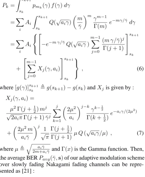
The mode-specific average BERPkis defined as :

Pk ,

Z sk+1

sk

pmk(γ)f(γ)dγ , (4)

wherepmk(γ)is the BER of themk-ary modulation scheme

over the AWGN channel. The BER of a Gray-coded square QAM scheme over AWGN channels can be expressed as [2, 19] :

pmk(γ) =

X

i

AiQ(

√

aiγ), (5)

whereAi andai are constants. The approximate BER of a

Gray-codedmk-ary coherent PSK (k ≥ 3) scheme over an

AWGN channel can also be expressed using (5) with the con-stants of A1 = A2 = 2/k, a1 = 2 sin2(π/mk)) and a2 =

2 sin2(3π/mk))[20]. Upon substituting (5) into (4), we have :

Pk =

Z sk+1

sk

pmk(γ)f(γ)dγ

=X

i

Ai

Z sk+1

sk

Q(√aiγ)

_m

¯

γ

m_γm₋1

Γ(m)e

−mγ/γ¯_dγ

=X

i

Ai

    −e−

m γ/γ¯_Q(√_a

iγ)

m−1

X

j=0

(m γ/γ¯)j Γ(j+ 1)

 

sk+1

sk

+

 

m−1

X

j=0

Xj(γ, ai)

 

sk+1

sk

  

, (6)

where[g(γ)]sk+1

sk ,g(sk+1)−g(sk)andXjis given by :

Xj(γ, ai) =

µ2_Γ(j+1 2)m

j

√

2aiπΓ(j+ 1) ¯γj j

X

k=1

_2µ2 ai

j−k_γk−1 2

Γ(k+1 2)

e−aiγ/(2µ2)

+

_2µ2_m ai¯γ

j ₁

√

π

Γ(j+1 2)

Γ(j+ 1)µ Q(

√

aiγ/µ) , (7)

whereµ_,q ai¯γ

2m+ai¯γ andΓ(x)is the Gamma function. Then,

the average BERPavg(¯γ,s)of our adaptive modulation scheme

over slowly fading Nakagami fading channels can be repre-sented as [21] :

Pavg(¯γ,s) = 1

B(¯γ,s)

K−1

X

k=0

3. OPTIMUM SWITCHING LEVELS

Our aim is to optimise the set of switching levels, s, so that the average BPS throughputB(¯γ;s)can be maximised under the constraint of Pavg(¯γ;s) = Pth, where Pth is the target

average BER. Let us definePRof aK-mode adaptive

modula-tion scheme as the weighted sum of the mode-specific average BER, namely asPR(¯γ;s) , P

K₋1

k=0 bk Pk, wherebk is the

BPS of thek-th constituent fixed-mode modem and the mode-specific average BERPkis given in (4). Then, with the aid of

(8), the average BER constraint can also be written as :

Pavg(¯γ;s) =Pth ⇐⇒ PR(¯γ;s) =PthB(¯γ;s). (9)

As we discussed before, our goal is to maximise our ob-jective function given by the average throughput of (2)B(¯γ;s)

under the constraint of (9). The set of switching levelsshas K+ 1 elements in it. However, since we stipulates0 = 0 andsK =∞in many adaptive modulation schemes, we have

K−1independent variables ins. Hence, the optimisation task is aK−1dimensional optimisation under an equality con-straint [17]. A standard practice is to introduce a modified ob-jective function using a Lagrangian multiplier and convert the problem into a set of one-dimensional optimisation problems. Hence the modified objective function Λ can be formulated employing a Lagrangian multiplierλas [17] :

Λ(s; ¯γ) =B(¯γ;s) +λ{PR(¯γ;s)−PthB(¯γ;s)} (10) = (1−λPth)B(¯γ;s) +λPR(¯γ;s). (11)

The optimum set of switching levels should satisfy :

∂Λ

∂s = 0 and PR(¯γ;s)−PthB(¯γ;s) = 0. (12)

The following relationships are readily derived, which are help-ful in evaluating the partial differentiations in (12) :

∂Pk−1 ∂sk

= ∂

∂sk

Z sk

sk−1

pmk−1(γ)f(γ)dγ=pmk−1(sk)f(sk)

∂Pk

∂sk

= ∂

∂sk

Z sk+1

sk

pmk(γ)f(γ)dγ=−pmk(sk)f(sk)

∂ ∂sk

Fc(sk) =

∂ ∂sk

Z ∞

sk

f(γ)dγ=−f(sk).

Using these results, the partial derivative ofPRandB against

skcan be expressed as :

∂PR

∂sk

=bk₋1pmk−1(sk)f(sk)−bkpmk(sk)f(sk) (13)

∂B ∂sk

=−ckf(sk), (14)

wherebk is the BPS throughput of anmk-ary modem andck

is the incremental BPS throughput defined asck ,bk−bk₋1 in Section 2. Hence, the first condition of∂Λ/∂s= 0in (12)

results in :

−ck(1−λ Pth)f(sk) +λ

bk−1pmk−1(sk)−bkpmk(sk) f(sk) = 0. (15)

A trivial solution of (15) isf(sk) = 0. However, the

cor-responding sk of either sk = ∞ or sk = 0in conjunction

with somef(γ)does not satisfy the second condition given in (12). Whenf(sk)6= 0, Equation (15) can be simplified upon

dividing both sides byf(sk), yielding :

ck(λ Pth−1)−λ

bkpmk(sk)−bk−1pmk−1(sk) = 0. (16)

Rearranging (16) fork= 1and assumingc16= 0, we have :

λ Pth−1 = (λ/c1){b1pm1(s1)−b0pm0(s1)} . (17)

Substituting (17) into (16) and assumingck 6= 0fork6= 0, we

have :

(λ/ck){bkpmk(sk)−bk−1pmk−1(sk)}

= (λ/c1){b1pm1(s1)−b0pm0(s1)}. (18)

We note that the Lagrangianλis not zero, because substitution ofλ = 0in (16) leads to−ck = 0for allk. Hence, we can

eliminate the Lagrangian multiplier dividing both sides of (18) byλ. Then we have :

yk(sk) =y1(s1) fork= 2,3,· · ·K−1, (19)

where the Lagrangian-free functionyk(sk)is defined as :

yk(sk),(1/ck)

bkpmk(sk)−bk−1pmk−1(sk) . (20)

The significance of (19) and (20) is that the relationship be-tween the optimum switching level sk , k 6= 1 ands1 is in-dependent of the underlying channel scenario. Only the con-stituent modulation mode related parameters, such asbk, ck

andpmk(γ), govern this relationship. Furthermore, since we

made no assumptions concerning the modulation modes em-ployed, (19) holds for generic adaptive modulation schemes.

It is straightforward to solve (19) numerically, in order to findsk as a function ofs1, since it is a one-dimensional root

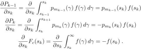
[image:3.595.46.287.525.609.2]

finding problem [16]. As an example, the relationship between the optimum switching levels of the 5-mode AQAM scheme is depicted in Figure 1(a) using the parameters summarised in Table 1,

Since we can relate the remaining switching levels tos1, we have to determine the optimum value of s1for the given target BER Pth using the PDF of the instantaneous channel

SNRf(γ)and the second condition given in (12). This prob-lem is also a one-dimensional root finding probprob-lem rather than a multi-dimensional optimisation problem, which was the case in [11, 15], where the latter sometimes settles in local minima. Let us define the constraint functionY(¯γ;s(s1))as :

-60 -50 -40 -30 -20 -10 0 10 switching levels1(dB)

-60 -40 -20 0 20 40

s

w

it

c

h

in

g

le

v

e

ls

{

si

}

(d

B

)

s4 s3 s2 s1 s4= 1.82 dB

asymptotic line

s3= -7.34 dB

(a) Relationship betweenskands1

-30 -25 -20 -15 -10 -5 0 5 10 15 switching levels1(dB)

-0.06 -0.04 -0.02 0.0 0.02 0.04

Y

(

s1

)

Pt=10 -6 Pt=10

-4 Pt=10

-3 Pt=10

-2.5 Pt=10

-2

locus of minY(s1)

Rayleigh channel average SNR = 30 dB

(b) Constraint functionY

0 5 10 15 20 25 30 35 40 Avrage SNR per symbol in dB -10

-5 0 5 10 15 20 25 30

S

w

it

c

h

in

g

le

v

e

ls

in

d

B

Rayleigh channel 5-mode AQAM, =10-3

No-Tx region BPSK region

QPSK region 16-QAM region

64-QAM region

[image:4.595.69.548.81.255.2]

(c) Optimised switching levels

Figure 1: Switching level optimisation for 5-mode AQAM. (a) There exists a fixed relationship between the optimum switching levelssk ands1, regardless of the underlying channel scenario. (b) The constraint equation of (9) has a unique solution, when

Y(¯γ,s(s1 = 0)) < 0. (c) The optimised switching levels forPth = 10−3. The switching levels of [15] are represented by

corresponding thin grey lines for comparison.

where we useds(s1) to emphasise thatsk is dictated by s1 according to the relationships of (19) and (20). Even though the relationship implied bys(s1)is independent of the channel conditions and of the signaling power, the constraint function Y of (21) and hence the actual values of the optimum switching levels are dependent on them through the PDFf(γ)of the SNR per symbol and through the average SNR per symbol¯γ.

The first derivative ofY0 =dY /ds1can be expressed as :

Y0= (b0pm0(s1)−b1pm1(s1)+Pth)

K₋1

X

k=1

ck

c1 f(sk)

dsk

ds1 . (22)

A further study ofY andY0revealed thatY has its first maxi-mum ats1= 0, its minimum, whenb1pm1(s1)−b0pm0(s1) =

Pth and its other asymptotic maximum of Y = 0− ats1 =

∞. Hence, when satisfying the second condition in (12) ex-pressed as Y = 0 we have a unique solution, provided that Y(¯γ;s(0))>0.

Figure 1(b) depicts the values ofY for 5-mode AQAM us-ing various target BERs ofPth, when the average channel SNR

is 30dB. We can observe thatY= 0may have a root depending on the target BERPth. Whensk= 0fork <5, the value ofY

becomes :

Y(¯γ; 0) = 6(P64(¯γ)−Pth), (23)

whereP64(¯γ)is the average BER of 64-QAM over a flat Ray-leigh channel. The value ofY(¯γ; 0) in (23) can be negative or positive, depending on the target BER Pth. Figure 1(c)

depicts the switching levels optimised in this manner for the 5-mode AQAM scheme achieving the target average BER of

10−3_{. The optimised switching levels obtained using Powell’s} minimisation method for each SNR [15] are represented as thin grey lines in Figure 1(c) for comparison. When using the Lagrangian optimisation, the various modulation modes are not abandoned, until the average SNR reaches the avalanche

SNR around 38dB, while Powell’s minimisation required the AQAM regime to abandon the lower-order modulation modes one by one, as the average SNR increased.

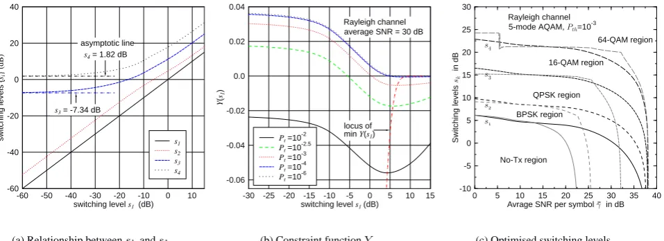
Figure 2(a) depicts the average BER performance of 5-mode AQAM employing the Lagrangian optimised switching levels operating over a Rayleigh channel. The average BER remains constant until the average SNR reaches the avalanche SNR, where the average BER of the highest-order constituent modulation mode, ie 64-QAM, satisfies the target average BER constraint. Figure 2(b) depicts the average BPS throughput B of the AQAM scheme employing the optimised switching levels. The average throughput of 6-mode AQAM using Tor-rance’s scheme [11] is represented by the thin grey line. The Lagrangian based scheme showed SNR gains of 0.6dB, 0.5dB, 0.2dB and 3.9dB at a BPS throughput of 1, 2, 4 and 6, respec-tively, compared to Torrance’s scheme. The average through-put of 6-mode AQAM is depicted in Figure 2(c) for the several values ofPthare, where the BPS values of the AQAM scheme

employing the switching levels optimised individually for each SNR value [15] using Powell’s method [16] are also repre-sented as thin lines forPth = 10−1,10−2 and10−3.

Com-paring the BPS curves, we conclude that the ‘per-SNR’ Powell optimisation method of [15] resulted in imperfect optimisation for some values of the average SNR. The schemes of [15] were unable to generate a reasonable set of switching levels leading to a monotonically increasing average BPS throughput for the target average value ofPth= 10−4and10−5.

4. CONCLUSION

aver-0 5 10 15 20 25 30 35 40 Avrage SNR per symbol in dB 10-6

10-5 10-4 10-3 10-2 10-1 100

A

v

e

ra

g

e

B

E

R

(

)

Rayleigh channel = 10-1

= 10-2

= 10-3

= 10-4

5-mode AQAM employing the optimised switching levels

(a) Average BER of the 5-mode AQAM

0 5 10 15 20 25 30 35 40 Avrage SNR per symbol in dB 0

1 2 3 4 5 6 7 8

A

v

e

ra

g

e

th

ro

u

g

h

p

u

t

(

)

in

B

P

S

6-mode 5-mode 4-mode 3-mode 2-mode Rayleigh channel AQAM, = 10-2

fixed QAM =

BPSK QPSK

16QAM 64QAM

256QAM

throughput of Torrance’s scheme

(b) Average BPS forPth= 10−2

0 5 10 15 20 25 30 35 40 Avrage SNR per symbol in dB 0

1 2 3 4 5 6 7 8

A

v

e

ra

g

e

th

ro

u

g

h

p

u

t

(

)

in

B

P

S

= 10-5 = 10-4 = 10-3 = 10-2 = 10-1 Rayleigh channel

6-mode AQAM

[image:5.595.65.548.82.250.2]

(c) Average BPS of the 6-mode AQAM

Figure 2: Performance of AQAM employing the optimised switching levels over a Rayleigh channel. (a) The average BER remains constant until the average SNR reaches the avalanche SNR, where the average BER of the highest modulation mode is down toPth. (b) The average throughput of the 6-mode AQAM using Torrance’s switching levels [11] is represented as a thin

grey line for comparison. (c) The average throughputs of the 6-mode AQAM employing per-SNR optimised switching levels [15] represented in thin lines forPth= 10−1,10−2and10−3only.

age throughput and of the average BER derived for transmis-sions over Nakagami fading channels, we presented numerical results for AQAM operating over a Rayleigh fading channel as an example. Compared to other existing switching level de-sign schemes, our technique exhibited superior performance. One of the advantages of our optimised constant-power adap-tive modulation systems is that it can be readily combined with other power control schemes in cellular environments, since our scheme does not require a transmit-power adjustment for maintaining optimal operation, unlike the variable-power, variable-rate AQAM schemes of [10].

5. REFERENCES

[1] R. Steele and L. Hanzo, eds., Mobile Radio Communications. New York, USA: IEEE Press - John Wiley & Sons, 2nd ed., 1999.

[2] L. Hanzo, W. T. Webb, and T. Keller, Single- and Multicarrier

Modula-tion; Principles and Applications for Personal Communications, WLANs and Broadcasting. IEEE Press, and John Wiley & Sons, 2000.

[3] J. F. Hayes, “Adaptive feedback communications,” IEEE Transactions

on Communication Technology, vol. 16, no. 1, pp. 29–34, 1968.

[4] J. K. Cavers, “Variable-rate transmission for Rayleigh fading chan-nels,” IEEE Transactions on Communication Technology, vol. 20, no. 1, pp. 15–22, 1972.

[5] W. T. Webb and R. Steele, “Variable rate QAM for mobile radio,” IEEE

Transactions on Communications, vol. 43, no. 7, pp. 2223–2230, 1995.

[6] R. Steele and W. T. Webb, “Variable rate QAM for data transmission over mobile radio channels,” in Keynote Paper, Wireless ’91, (Calgary, Alberta), June 1991.

[7] S. Otsuki, S. Sampei, and N. Morinaga, “Square QAM adaptive modula-tion/TDMA/TDD systems using modulation level estimation with Walsh function,” Electronics Letters, vol. 31, pp. 169–171, February 1995.

[8] W. C. Y. Lee, “Estimate of channel capacity in Rayleigh fading environ-ment,” IEEE Transactions on Vehicular Technology, vol. 39, pp. 187– 189, August 1990.

[9] A. J. Goldsmith and P. P. Varaiya, “Capacity of fading channels with channel side information,” IEEE Transactions on Information Theory, vol. 43, pp. 1986–1992, November 1997.

[10] A. J. Goldsmith and S.-G. Chua, “Variable rate variable power MQAM for fading channels,” IEEE Transactions on Communications, vol. 45, no. 10, pp. 1218–1230, 1997.

[11] J. M. Torrance and L. Hanzo, “Optimization of switching levels for adap-tive modulation in a slow Rayleigh fading,” Electronics Letters, vol. 32, pp. 1167–1169, 20 June 1996.

[12] C.-H. Wong and L. Hanzo, “Upper-bound performance of a wide-band adaptive modem,” IEEE Transactions on Communication Technology, vol. 48, no. 3, pp. 367–369, 2000.

[13] E. L. Kuan and L. Hanzo, “Burst-by-burst adaptive joint detection CDMA,” in Proc. IEEE VTC’99 Fall, vol. 2, pp. 1628–1632, IEEE, September 1999.

[14] T. Keller and L. Hanzo, “Adaptive modulation technique for duplex OFDM transmission,” IEEE Transactions on Vehicular Technology, vol. 49, pp. 1893–1906, September 2000.

[15] B.-J. Choi, M. M¨unster, L.-L. Yang, and L. Hanzo, “Performance of RAKE receiver assisted adaptive-modulation based CDMA over fre-quency selective slow Rayleigh fading channel,” Electronics Letters, vol. 37, pp. 247–249, February 2001.

[16] W. H. Press, S. A. Teukolsky, W. T. Vetterling, and B. P. Flannery,

Nu-merical Recipies in C. Cambridge University Press, 1992.

[17] G. S. G. Beveridge and R. S. Schechter, Optimization: Theory and

Prac-tice. McGraw-Hill, 1970.

[18] M. Nakagami, “Them-distribution - A general formula of intensity dis-tribution of rapid fading,” in Statistical Methods in Radio Wave

Propa-gation (W. C. Hoffman, ed.), pp. 3–36, Pergamon Press, 1960.

[19] D. Yoon, K. Cho, and J. Lee, “Bit error probability of M-ary Qadrature Amplitude Modulation,” in Proc. IEEE VTC 2000-Fall, vol. 5, pp. 2422– 2427, IEEE, September 2000.

[20] J. Lu, K. B. Letaief, C.-I. J. Chuang, and M. L. Lio, “PSK and M-QAM BER computation using signal-space concepts,” IEEE

Transac-tions on CommunicaTransac-tions, vol. 47, no. 2, pp. 181–184, 1999.