A. RSS Based Positioning Systems

Abstract—The work presented here compares the performance of indoor positioning systems suitable for low power wireless sensor networks. Map matching, approximate positioning (weighted centroid) and exact positioning algorithms (least squares) were tested and compared in a small predefined indoor environment. We found that, for our test scenario, weighted centroid algorithms provided the best results. Least squares proved to be completely unreliable when using distances obtained by a propagation model. Major improvements in the positioning error were found when body influence was removed from the test scenario.

Index Terms— Fingerprinting, localization, received signal strength, wireless sensor networks, weighted centroid.

I. INTRODUCTION

OCALIZATION capability in wireless sensor networks (WSN) brings spatial information to data obtained from sensors. A device’s ability to provide localization information enables numerous added value applications. Localization can be used in the most various contexts, from geodesic routing to antenna beam forming, or to detect soil temperature and pinpoint the origin of a wildfire.

In outdoors environment, the global positioning system (GPS) is capable of offering an adequate service to the majority of applications. Device size is no longer an issue in WSN due to the miniaturization of GPS hardware. Remaining disadvantages of this approach relate to energy consumption and node price when using this technology in WSN.

Regarding indoors environment, GPS is not reliable due to the signal attenuation. Ultra-wideband is a technology with potential to solve the problem of indoor location due to its high accuracy when inferring distances between devices [1]. However, and despite large standardization efforts (e.g., the IEEE 802.15.4a standard), a fully compliant commercial device for sale is unavailable. Since no mass market is

Manuscript sent March 20, 2014; revised April 2, 2014. This work is supported by the Portuguese Foundation for Science and Technology (FCT) in the scope of the project PEst-OE/EEI/UI0319/2014. Helder D. Silva is supported by FCT under the grant SFRBD/7080/2011.

Helder D. Silva is with Centro Algoritmi, Department of Industrial Electronics, University of Minho, Campus of Azurem 4800-058 Portugal (phone: +351-912-457-225; e-mail: helderdavidms@ gmail.com).

José A. Afonso is also with the Department of Industrial Electronics, University of Minho, Campus of Azurem, 4800-058 Portugal. (e-mail: [email protected]).

Luís A Rocha is also with the Department of Industrial Electronics, University of Minho, Campus of Azurem, 4800-058 Portugal. (e-mail: [email protected]).

currently in place, prices are very high.

Received signal strength (RSS) based positioning is a popular approach in WSNs since RSS is readily available with the radio module. Due to typical WSN energy consumption and computational capacity constraints, low complexity positioning solutions are desired. As such, researchers seek to find balance between accuracy and computational complexity.

The aim of the work presented here is the implementation of positioning systems (PS) in WSN that best fit the indoor scenario. In this paper, a practical implementation of RSS based positioning using wireless sensor nodes is presented. The wireless sensor nodes communicate using the IEEE 802.15.4 medium access control (MAC) protocol, working on the 2.4 GHz frequency band. We compare positioning calculation using map matching, approximate positioning and exact positioning algorithms in an indoor test scenario. We also study the effect of the body in the performance indicators.

Map matching solutions are mainly used in large areas, such as office settings and warehouses with several divisions. Our work differs from the usual approach, since the fingerprinting solution is implemented in a smaller predefined space of a room, without walls in between access points, according to our setup.

We seek to study positioning techniques that are compatible with real-time positioning in WSN, having low-power and low complexity as requirements, yet presenting the best accuracy possible under such framework.

II. BACKGROUND

A. RSS Based Positioning Systems

An overview of technologies used in positioning systems is available in [2]. Ultrasound, ultra-wideband, radio-frequency identification (RFID) and RSS based systems are among the most used technologies for indoor positioning. Accuracies span from 5 meters (RSS) to a few centimeters (ultrasound).

RSS systems are known for the low reliability when inferring distances from measurements. Filtering techniques are a solution for dealing with RSS reliability under noisy conditions. These techniques also stand as the common solution for integration of heterogeneous positioning systems, in order to provide more accurate location estimation. Kalman filters [3] and particle filters [4] are the usual approaches; however, since these solutions need high computational capacity, they are usually not compatible

Experimental Performance Comparison of

Indoor Positioning Algorithms based on

Received Signal Strength

Helder D. Silva, José A. Afonso, and Luís A. Rocha

with WSNs. Instead, filtering is typically accomplished by averaging multiple measurements, thus positioning accuracy is sacrificed in the tradeoff for lower computational demands, longer lifespan of sensor nodes and faster positioning update rates when desired.

Map matching systems are a popular approach in RSS positioning in wireless local area networks (WLANs). Approximate positioning uses radio parameters such as link quality indication (LQI), RSS or node connectivity to infer proximity to a certain known reference point. Exact positioning systems use RSS readings as input for mathematical models that estimate distances between devices in a network.

B. Propagation Models

A general overview of various propagation models can be found in [5]. Several efforts have been made to characterize radio signal propagation during the GSM (Groupe Special Mobile) system’s evolution, through the COST 231 project [6]. For indoor settings, the one-slope [7] and the multiwall [8] propagation models are frequently used in the state-of-the-art. The one-slope model is defined as:

RSS_OS(d)=RSS(d₀)−10×n×log d d₀

#

$

%

&

'

(

+

χ

_σ (1)

The parameter RSS(d0) is the received signal strength at the reference distance d0 (usually 1 meter), n is the path loss exponent and χσ is a Gaussian distributed random variable.

The propagation model typically models the large-scale effects of signal attenuation. The main error source comes from the small-scale fading effect. Multipath waves combine at the receiver in slightly different time instants, giving rise to a signal that can largely vary in amplitude and phase [9].

A path loss exponent of 2 is the reference path loss, used in free space propagation. Authors in [10] and [11] obtained path loss exponent values above 2, typical in non-line-of-sight (NLOS) or reflection dominated environments. Values below 2 are less frequent but sometimes found in literature [8].

When devices are worn near or on the human body, propagation models performance degrades. In [12], attenuations as high as 15dB due to human body are reported when compared to the line-of-sight (LOS) case. Body attenuation is of extreme importance, yet a model that incorporates the body effect has not been investigated in the literature.

C. Map Matching

Two phases compose the system originally implemented by Bahl et al. [13]. In the offline phase, data relating position and RSS from access points (AP) is gathered from the site on to a database, in order to create a radio map. In the online phase, mobile nodes report to a server the RSS from APs in range. The server compares signatures so a match (or the closest to) can be found, thus pinpointing the mobile node’s position.

In [14], a comprehensive study on fingerprinting is presented. Authors conclude that map density translates to higher accuracy with a nonlinear behavior in increasing the number of calibration points. The direction faced when

collecting samples, also studied by Bahl et al., is crucial and greatly improves system accuracy.

Approaches to facilitate creation of radio map in the offline phase have been conducted. Authors in [11] use propagation models to ease the process of creating the radio map. Ray-tracing modeling is another solution to obtain the attenuation values of signal propagation [15].

D. Approximate Positioning

This method involves determining the proximity when a device or object is near a known location.

The weighted centroid localization (WCL) method is a well-known, low complexity algorithm with good robustness to noise. Bulusu et al. implemented this method in [16], were node connectivity was the metric used to infer distance. Given a set of beacon nodes in the network possessing knowledge of their location, the position of sensor nodes can be estimated by calculating the centroid of all beacon node coordinates for which the sensor is in range of.

In [17], authors compare the linear least squares (LLS) method against centroid-based algorithms. Results show that centroid based method outperforms the LLS method in precision and accuracy with lower complexity, when under an environment strongly affected by multipath propagation.

LANDMARC [18] uses RSS readings in their approximate positioning method. Tag readers report RSS from RFID moving tags, along with RSS from reference tags. Reference tags are fixed and their RSS are used as means of comparison between that of the movable tags to infer proximity. In a more recent work [19] authors further improve LANDMARC’s positioning error to a 1-meter accuracy with a signal reporting cycle of 2 seconds.

Hop count positioning algorithms such as DV-Hop [20] can use RSS as a metric to infer distance for each hop. In [21], authors achieve less than 10% radio coverage error. In contrast with [21], authors in [22] discard a RSS solution due to its low reliability. These contradictory opinions are strongly related to the use case scenario of each positioning system implementation.

E. Exact Positioning

The exact positioning method involves the determination of angles or distances between a sensor node and multiple known reference points. Triangulation and trilateration (or multilateration) are the typical methods employed to determine the sensor position. Distance estimates are usually obtained by measuring the time of arrival (TOA), time difference of arrival (TDOA) or the round trip time of flight (RTOF) [23].

The linear least squares method (LLS) [24] is the most used exact positioning algorithm in WSNs, due to the simple closed form solution.

III. MATERIALS AND METHODS

A. Hardware

Texas Instruments CC2530DK development kit was used in this work. The CC2530 is a system on chip (SoC) solution that contains an 8051 microprocessor, a radio transceiver compatible with the IEEE 802.15.4 MAC working on the 2.4GHz frequency band and general I/O (Input / Output) peripherals. The CC2530 radio has a sensitivity of -97 dBm and a maximum transmission power of +4.5 dBm.

The test scenario is composed by four anchor nodes and one sensor node. Each anchor node is composed by a CC2530 evaluation module and a battery board powered by two AA batteries. The sensor node is composed by a development board and an evaluation module. The development board contains necessary hardware to interface with the USART (Universal Synchronous Asynchronous Receiver Transmitter), used to communicate through standard PC serial port.

B. Experimental Setup

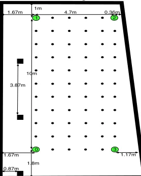
The anchor’s role is to broadcast beacon messages periodically, so sensor nodes can receive these messages and locate themselves. Our main test bed is a room with 10×4.7 m free space area, as shown in fig. 1.

Anchors are placed in the corners of the mentioned area on top of a stand, 1.2 meters above ground. The stands used are made of plastic, so no extra interferences affect the radio messages.

Numbered from 0 to 3, each anchor broadcasts one beacon message periodically, at the start of each 100-millisecond superframe. As soon as anchor 1 receives beacon message from anchor 0, anchor 1 begins broadcasting its own beacon periodically, and so forth. Anchor nodes bypass the usual CSMA/CA (Carrier Sense Multiple Access/Collision Avoidance) in their transmissions, so timings between transmissions do not overlap. Messages arrive sequentially and free of collision.

Using the sequence number in the beacon messages, the sensor node detects lost beacons during data collection and inserts a value of -127, indicating an invalid RSS sample. Calculations are performed in an offline phase.

C. Propagation Model Calibration

Equation 1 was used as the linear (in the coefficients) non-polynomial model, to find the parameters of the one-slope model:

M(x)=c₁φ₁(x)+c₂φ₂(x)+...+c_nφ_n(x) (2)

with ϕ1=1 and ϕ2=10×log10(x), where a reference distance of 1 meter was used. The model coefficients are calculated by minimizing the squared error between the model and the measurements taken at the site:

S=∑_iN₌₁

(

f_i−M(x_i)

)

2 (3)

The solution is found by solving a system of equations in augmented matrix form:

φ1 2

i=1

N

∑ i=1φ1φ2

N

∑ i=1f_iφ1

N

∑

φ₂φ₁ i=1

N

∑ i=1φ₂2 N

∑ i=1f_iφ₂ N

∑

"

#

$

$

%

&

'

'

(4)

D. Map Matching

The radio map was created with a grid resolution of one squared meter. Since our positioning area is 4.7 meters wide, the last column of the grid has a smaller resolution of 0.7 squared meters. A total of 66 grid points covered our test field. A calibration point was collected at each grid point and for each body orientation (e.g., north, west, south and east), amounting to a total of 264 calibration points. Each point is composed by true position (x and y with origin on anchor 0), body orientation and average RSS obtained from 100 RSS samples from all four anchor nodes.

During the online phase, the sensor node obtains RSS samples and stores them. At the end of a test run (e.g.: after collecting 100 samples), data is uploaded to the PC running MATLAB and the position is computed. The weighted k-nearest neighbor (WKNN) algorithm [13] uses (5) to find the distance in signal space between a RSS sample and each calibration point.

D_SS = i=1R_map(i)−R_s(i)p N

∑

#

$

%

&

1

p

(5) N is the number of anchor nodes in range and p is the norm used. The Rmap(i) is the RSS stored for anchor i in a calibration point of the radio map and Rs(i) is the RSS sampled in the online phase for anchor i. After computing the distances for all calibration points, the K smallest distances are used to estimate the node’s position using (6), with pi being the coordinates of each calibration point.

ˆ

x= wi×

 p_i i=1

K ∑

w_i i=1

K

∑ ; wi=

1

D₁

(6) The weight applied to each neighbor found in the search process is simply the inverse of the signal space distance.

E. Approximate Positioning

In this type of positioning, the only information needed by a node to calculate its position is the coordinates of each anchor node in range. The position estimate is calculated using (7):

ˆ

x= wi×  L_i i=1 B ∑

w_i i=1 B

∑ ; wi=

1

(R_p)e (7)

where Li are the coordinates of each anchor node and Rp

10m

4.7m

1.17m 1.67m

1.8m 1m

0

1 2

3

0.87m

1.67m 0.36m

[image:3.595.97.236.360.534.2]

3.87m

is the radio parameter used to calculate the weight. In this work, both the RSS and the distance using a propagation model were used to calculate the weights, in two different approaches. The exponent e allows an adjustment of the importance of the weight applied to each anchor node’s RSS.

F. Exact Positioning

The Linear Least Squares method is an exact positioning technique, which computes the position of a node using a set of three or more non-collinear distance measurements (in the two dimensional case). Each measurement produces an equation of the form illustrated in (8):

(x−x_n)2+(y−y_n)2 =d_n2 (8) Several measurements produce a system of equations, which has no solution when circles don’t intersect. To find a solution to this system, first a linearization of the system of equations is obtained by subtracting the location of the first anchor node from other locations. This cancels the unknown squared terms, and a linear system of the form Av = b is obtained, as shown in (9), (10) and (11):

A=2×

x₁−x₂ x₁−x₃ yy1₁−−yy2₃

...

x₁−x_n y₁...−y_n

#

$

%

%%

&

'

(

((

(9)

b=

d₂2−d₁2+x₁2−x₂2+y₁2−y₂2 d₃2−d₁2+x₁2−x₃2+y₁2−y₃2

...

d_n2−d₁2+x₁2−x_n2+y₁2−y_n2

"

#

$

$

$

$

%

&

'

'

'

'

(10)

v=

( )

x_y (11)

Since the vector b may be located outside the plane defined by matrix A, the solution is to find the projection of

b onto A, thus minimizing the Euclidean distance (or squared error), using (12).

v=(AT×A)−1×(AT×b) (12)

IV. RESULTS

One aspect of RSS positioning essential to its performance is the body influence. Two sets of samples were collected, with one set being obtained with the user’s body near the receiving antenna (body present BP), the other set without the body influence (body not present BNP). A set is composed by several test runs; each test run contains 100 RSS samples. Position estimation is computed for each sample in a test run, thus no averaging was used in the tests presented.

All sample sets were taken in positions where a calibration point exists. The BP sample set is composed by 79 test runs, from which 66 were taken facing the north direction. The remaining 13 test runs were randomly chosen across the positioning area, with different orientations. The BNP sample set is composed by 12 test runs randomly chosen and do not have an orientation associated since the body is not present.

The height of the sensor nodes is the same as the anchor nodes (1.2 meters above ground). The mean and standard

deviation of the absolute error (Euclidean distance between the calculated position and the true position) were the metrics chosen as primary performance indicators. Performance evaluation results and comparison between each algorithm are presented.

A. Propagation Model Calibration

The one-slope propagation model uses two parameters: the RSS at the reference distance and the path loss exponent. A reference distance of 1 meter was used, which simplifies computation of distances by the low power sensor nodes.

We collected twelve datasets of RSS measurements at different distances from each of the anchors and applied (2), (3) and (4) to find the one-slope model parameters. Table 1 presents the data collected.

The average value of each coefficient was used in our propagation model, presented in (13).

RSS_OS(d)=−37.72−10×2.19×log₁₀(d)+χ_σ (13) The RSS measurements for the propagation model were done with the body near the receiving antenna, and in LOS to each anchor node, which is the typical application scenario.

B. Map Matching

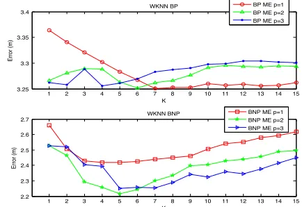
Two parameters were tested in the map matching solution: the number of neighbors K and the norm used p. The mean error (ME) and the standard deviation (STD) are presented in fig. 2 and fig. 3 respectively.

1 2 3 4 5 6 7 8 9 10 11 12 13 14 15

3.25 3.3 3.35 3.4

K

Error (m)

WKNN BP BP ME p=1

BP ME p=2 BP ME p=3

1 2 3 4 5 6 7 8 9 10 11 12 13 14 15

2.2 2.3 2.4 2.5 2.6 2.7

K

Error (m)

[image:4.595.316.533.576.725.2]

WKNN BNP BNP ME p=1 BNP ME p=2 BNP ME p=3

Fig. 2. Mean error comparison for different values of K and p. At the top is displayed the WKNN BP, at the bottom is displayed the WKNN BNP.

TABLEI

PROPAGATION MODEL MEASUREMENTS

Dataset RSS at distance d0 Exponent n

1 -30.88 3.88

2 -45.91 0.12

3 -32.18 1.81

4 -31.06 2.76

5 -36.09 3.17

6 -55.19 -0.16

7 -20.42 3.99

8 -34.76 2.72

9 -34.82 2.38

10 -47.71 1.40

11 -48.75 1.41

12 -34.84 2.74

Average -37.72 2.19

The body influence is presented for each of the p-norms tested. In the BP case, the ME variation between K=1, equivalent to the nearest neighbor (NN) algorithm, and the other values of K is not significant. This can be explained due to the positioning system area and calibration point density. Since the area is small and the density of calibration points is high, the NN algorithm tends to perform as good as WKNN. Other works, such as [14], also pointed out this outcome, yet under a different environment. Note that a map matching solution with NN as the positioning algorithm only needs to find one nearest neighbor, which is computationally faster than the WKNN case.

In the BNP case, the value K has a more important influence than in the BP case, where for p=2 and K=5, ME reaches a minimum of approximately 2.2 meters. This scenario were body influence is not present is, of course, a best-case scenario, which does not happen when the system is to be used by a person. Yet, it shows a boundary of positioning error that deterministic frameworks can provide in this environment, if accounting the body influence in the position calculation.

The STD values exhibit a monotonic decrease, with the increase of K in the BP case. Differences between norms are negligible. In the BNP case, STD values reach a minimum of 0.8 meters for p=1 and K=4.

C. Approximate Positioning

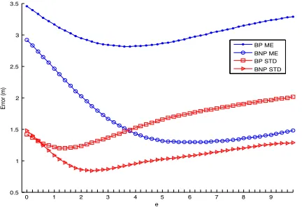
RSS (RWCL) and distance using the one-slope path loss model (DWCL) are tested as weights in the WCL algorithm. In the RWCL, the exponent e was varied. Results are presented in fig. 4.

In contrast with other works [25], [26], we found the optimum e parameter between 2 (BP) to 6 (BNP), where a tradeoff between the mean error and the standard deviation exists. As the parameter e increases beyond 4 in the BP case, and beyond 6 in the BNP case, the mean error and standard deviation also increase. With a high e value, the position is strongly influenced by the anchor node with the greater RSS reading. Thus, in limit conditions, the calculated position would be the same as that of the anchor node with higher RSS in the field.

Again, body influence plays a very important role. As an example, for an exponent of e=4, the mean error in the BNP case is approximately half of the mean error in the BP case. In the case of standard deviation, an improvement of more than 50% in the BNP case is also achieved.

In the DWCL algorithm, two parameters can be varied: exponent e and the path loss exponent n. Mean error and standard deviation results are presented in fig. 5 and 6.

The minimum ME of 1.36 meters is achieved (n=2.2, e=1.4) in the BNP case, while in the BP case, minimum ME was 2.92 meters (n=3.4, e=1). Body influence increases the error by a factor slightly higher than 2.

There is a balance between parameters, due to n and e balancing each other, which can be seen as the “saddle” effect in fig. 5 and 6.

The value of n=2.2 obtained in the BNP case is also very similar to the value obtained by linear regression of n=2.19, which validates the use of linear regression as an appropriate method of determining path loss exponent when in LOS conditions.

0 2

4 6

8

0 2 4 6 8 10 12 0.5 1 1.5 2 2.5 3

e DWCL STD

n

Error (m)

BP STD BNP STD

1 1.2 1.4 1.6 1.8 2 2.2 2.4 2.6

Fig. 6. DWCL standard deviation comparison for different values of the path loss exponent n and parameter e.

0 2

4 6

8

0 2 4 6 8 10 12

1 1.5 2 2.5 3 3.5 4 4.5

e DWCL ME

n

Error (m)

BP ME BNP ME

1.5 2 2.5 3 3.5 4

Fig. 5. DWCL mean error comparison for different values of the path loss exponent n and parameter e.

1 2 3 4 5 6 7 8 9 10 11 12 13 14 15 1.6

1.8 2 2.2 2.4

K

Error (m)

WKNN BP BP STD p=1 BP STD p=2 BP STD p=3

1 2 3 4 5 6 7 8 9 10 11 12 13 14 15 0.8

1 1.2 1.4 1.6

K

Error (m)

[image:5.595.61.277.49.197.2]

WKNN BNP BNP STD p=1 BNP STD p=2 BNP STD p=3

Fig. 3. Standard deviation comparison for different values of K and p. At the top is displayed the WKNN BP, at the bottom is displayed the WKNN BNP.

0 1 2 3 4 5 6 7 8 9 0.5

1 1.5 2 2.5 3 3.5

e

Error (m)

RWCL

[image:5.595.316.535.271.420.2]

BP ME BNP ME BP STD BNP STD

[image:5.595.321.534.456.602.2] [image:5.595.63.279.616.764.2]

D. Exact Positioning

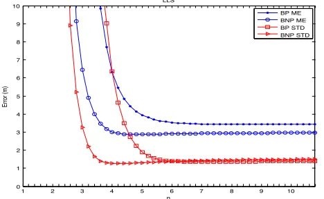
[image:6.595.309.541.101.253.2]

The influence of the parameter n of the one-slope model was tested. The results for the LLS algorithm are depicted in fig. 7.

Even though the mean error and the standard deviation decrease has n increases, the algorithm exhibits a saturated behavior, has can be seen for values of n higher than 6. Positioning error increases rapidly for values of n smaller than 4. For a value of n=2.19, as obtained for our one-slope model, the ME rises to around 1000 meters, many orders higher than the positioning area itself, which renders the algorithm useless.

E. Algorithm Comparison

In order to compare the several positioning algorithms, the best parameter values for each of the algorithms were considered.

To evaluate the algorithm’s sensitivity to noisy measurements, a simple simulation was made: given a set of positions (x, y) from our test setup, the real distance from all anchor nodes to each position was calculated. An error was added to this calculated distance and served as input to each algorithm that uses distances. For the RSS based algorithms, distances were converted to RSS using the inverse of (13). Results are presented in fig. 8.

Only the LLS algorithm exhibits zero error under exact distance estimates. Error increases rapidly with noise in the LLS case, while the other algorithms exhibit resilience to increasingly erroneous estimates.

To have a frame of reference when comparing algorithms, a fictitious positioning algorithm, called static center

position (SCP) was added to each CDF plot. This algorithm simply returns the center position of the PS area, for any input. The CDF for WKNN and LLS algorithms is presented in fig. 9.

The CDF for RWCL and DWCL algorithms is presented in fig. 10.

Regarding the WKNN algorithm, the body influence is evident, with a 30% improvement for an error of 3 meters.

The body has a bigger impact on WCL than in the map matching solution, yet the WCL algorithms present slightly better results than WKNN when under body influence. When body is not present, WCL produces the best position estimates of all algorithms tested. Considering a probability of around 70%, WCL improves from an accuracy of 4 meters in the BP case to approximately 1.8 meters in the BNP. Between RWCL and DWCL, different parameter values lead to an equivalent performance. This implies that the use of RSS is the best weighting solution in WCL for our setup, since it is simpler than using a propagation model.

LLS had the worst performance, where the BNP case obtained a performance at the same level of the BP case for the other algorithms. When compared with SCP, LLS can even sometimes perform worse.

In general, all algorithms exhibited weak performances when the body is present. If the body influence is removed, WCL algorithms can perform significantly better than WKNN. In addition to this, WCL also has reduced complexity, easier setup and maintenance than WKNN. Little overhead is needed to allow nodes to compute their position, since nodes only need to know the coordinates of the anchor nodes.

1 2 3 4 5 6 7

0 0.1 0.2 0.3 0.4 0.5 0.6 0.7 0.8 0.9 1

Error (m)

Cumulative probability

WKNN and LLS overall comparison

[image:6.595.53.287.117.261.2]

LLS BP n=9 WKNN BNP k=5 p=2 LLS BNP n=4.8 SCP WKNN BP k=1 p=2

Fig. 9. Cumulative Distribution Function for WKNN and LLS algorithms.

0 2.5 5 7.5 10 12.5 0

1 2 3 4 5 6 7 8 9 10

Mean Error (m)

Error (m)

Error Resilience

[image:6.595.308.542.271.455.2]

WKNN ME RWCL ME DWCL ME LLS ME WKNN STD RWCL STD DWCL STD LLS STD

Fig. 8. Error resilience comparison between algorithms tested.

1 2 3 4 5 6 7 8 9 10 0

1 2 3 4 5 6 7 8 9 10

n

Error (m)

LLS

BP ME BNP ME BP STD BNP STD

Fig. 7. LLS comparison using different values of path loss exponent n for distance conversion.

[image:6.595.49.287.544.701.2]

V. DISCUSSION

The comparison between the results obtained for the BP and BNP case demonstrate how strong the body influence is. Given the results, it is of extreme importance to account for body influence when estimating the position using RSS.

The use of propagation models proved to be unreliable in the case of the LLS algorithm.

Although more information from the propagation environment is embedded in the map matching solution, the results obtained did not compensate such effort when compared to WCL algorithm.

The performance obtained from the WCL solutions is equivalent to the map matching solution in the BP case. WCL solutions provided the best position estimates in the BNP case, making this type of positioning the best possible under our test conditions.

All algorithms showed poor positioning capabilities when body influence is present. When body influence is removed, positioning accuracy improves drastically, with the exception of LLS.

VI. CONCLUSIONS AND FUTURE WORK

Propagation models perform poorly due to not accounting for body influence and when the environment is severely affected by multipath propagation. Distances estimated from these models are severely affected by biases that heavily depend on factors such as body orientation, LOS/NLOS condition and proximity to other objects, walls or obstructions.

As future work, we intend to integrate the RSS indoor positioning capability in our wireless posture monitoring system (WPMS) [27]. The objective is to provide location information, which, together with the body posture, will characterize not only how the user is moving but also his location. The information sensed from the users body will be used to aid in the positioning task.

REFERENCES

[1] E. Karapistoli, F.-N. Pavlidou, I. Gragopoulos, and I. Tsetsinas, “An overview of the IEEE 802.15.4a Standard,” IEEE Commun. Mag., vol. 48, no. 1, pp. 47–53, Jan. 2010.

[2] T. K. Kohoutek, R. Mautz, and A. Donaubauer, “Real-time Indoor Positioning Using Range Imaging Sensors,” in Proceedings of SPIE Photonics, 2010, vol. 7724, no. May, p. 77240K–77240K–8. [3] G. Glanzer, T. Bernoulli, T. Wiessflecker, and U. Walder,

“Semi-autonomous indoor positioning using MEMS-based inertial measurement units and building information,” 2009 6th Work. Positioning, Navig. Commun., vol. 2009, pp. 135–139, Mar. 2009. [4] H. Wang, H. Lenz, A. Szabo, J. Bamberger, and U. D. Hanebeck,

“WLAN-Based Pedestrian Tracking Using Particle Filters and Low-Cost MEMS Sensors,” 2007 4th Work. Positioning, Navig. Commun., vol. 2007, pp. 1–7, Mar. 2007.

[5] I. Forkel and M. Salzmann, “Radio Propagation Modelling and its Application for 3G Mobile Network Simulation,” 10th Aachen Symp. Signal Theory, pp. 363–375, 2001.

[6] E. Damosso and L. M. Correia, Cost 231 Final Report: Digital Mobile Radio Towards Future Generation Systems. 1999.

[7] Z. Zhang, G. Wan, M. Jiang, and G. Yang, “Research of an adjacent

correction positioning algorithm based on RSSI-distance

measurement,” 2011 Eighth Int. Conf. Fuzzy Syst. Knowl. Discov., pp. 2319–2323, Jul. 2011.

[8] S.-Y. Yeong, W. Al-Salihy, and T.-C. Wan, “Indoor WLAN Monitoring and Planning Using Empirical and Theoretical Propagation Models,” 2010 Second Int. Conf. Netw. Appl. Protoc. Serv., pp. 165–169, Sep. 2010.

[9] T. S. Rappaport, Wireless Communications: Principles and Practice. Englewood Cliffs, New Jersey: Prentice-Hall, 1996.

[10] L. C. Liechty, E. Reifsnider, and G. Durgin, “Developing the Best 2 . 4 GHz Propagation Model from Active Network Measurements,” in IEEE 66th Vehicular Technology Conference, 2007, no. 404, pp. 894–896.

[11] P. Mestre, L. Coutinho, L. Reigoto, J. Matias, and C. Serodio, “Hybrid technique for Fingerprinting using IEEE802 . 11 Wireless Networks,” in International Conference on Indoor Positioning and Indoor Navigation, 2011, no. September.

[12] E. Miluzzo, X. Zheng, K. Fodor, and A. T. Campbell, “Radio Characterization of 802.15.4 and Its Impact on the Design of Mobile Sensor Networks,” in 5th European Conf. on Wireless Sensor Networks (EWSN ’08), 2008, pp. 171–188.

[13] P. Bahl and V. N. Padmanabhan, “RADAR: An in-building RF-based user location and tracking system,” in INFOCOM 2000. Nineteenth Annual Joint Conference of the IEEE Computer and Communications Societies. Proceedings. IEEE, 2000, vol. 2, pp. 775 – 784 vol.2. [14] V. Honkavirta, T. Perala, S. Ali-Loytty, and R. Piche, “A comparative

survey of WLAN location fingerprinting methods,” in 2009 6th Workshop on Positioning, Navigation and Communication, 2009, vol. 2009, pp. 243–251.

[15] A. V. Bosisio and C. N. R. Ieiit, “Performances of an RSSI-based positioning and tracking algorithm,” in International Conference on Indoor Positioning and Indoor Navigation, 2011, no. September. [16] N. Bulusu, J. Heidemann, and D. Estrin, “GPS-less low-cost outdoor

localization for very small devices,” Pers. Commun. IEEE, vol. 7, no. 5, pp. 28–34, 2000.

[17] A. Fink and H. Beikirch, “Analysis of RSS-based Location Estimation Techniques in Fading Environments,” in International Conference on Indoor Positioning and Indoor Navigation, 2011, no. SEPTEMBER.

[18] L. M. Ni, Y. Liu, Y. C. Lau, and A. P. Patil, “LANDMARC: Indoor Location Sensing Using Active RFID,” Wirel. Networks, vol. 10, no. 6, pp. 701–710, Nov. 2004.

[19] X. Yinggang, K. JiaoLi, W. ZhiLiang, and Z. Shanshan, “Indoor location technology and its applications base on improved LANDMARC algorithm,” 2011 Chinese Control Decis. Conf., no. 2, pp. 2453–2458, May 2011.

[20] S. Tian, X. Zhang, P. Liu, P. Sun, and X. Wang, “A RSSI-Based DV-Hop Algorithm for Wireless Sensor Networks,” 2007 Int. Conf. Wirel. Commun. Netw. Mob. Comput., pp. 2555–2558, Sep. 2007. [21] R. Nagpal, H. Shrobe, and J. Bachrach, “Organizing a Global

Coordinate System from Local Information on an Ad Hoc Sensor Network,” in Proceedings of the 2nd international conference on Information processing in sensor networks, 2003, pp. 333–348. [22] C. Savarese, J. Rabaey, and K. Langendoen, “Robust Positioning

Algorithms for Distributed Ad-Hoc Wireless Sensor Networks,” in ATEC ’02 Proceedings of the General Track of the annual conference on USENIX Annual Technical Conference, 2002, pp. 317–327.

[23] J. Hightower and G. Borriello, “A Survey and Taxonomy of Location Systems for Ubiquitous Computing,” 2001.

[24] A. Savvides, C.-C. Han, and M. B. Strivastava, “Dynamic fine-grained localization in Ad-Hoc networks of sensors,” Proc. 7th Annu. Int. Conf. Mob. Comput. Netw. - MobiCom ’01, pp. 166–179, 2001. [25] J. Blumenthal, R. Grossmann, F. Golatowski, and D. Timmermann,

“Weighted Centroid Localization in Zigbee-based Sensor Networks,” 2007 IEEE Int. Symp. Intell. Signal Process., pp. 1–6, 2007. [26] F. Reichenbach and D. Timmermann, “Indoor Localization with Low

Complexity in Wireless Sensor Networks,” 2006 IEEE Int. Conf. Ind. Informatics, pp. 1018–1023, Aug. 2006.