The Effect of Material Property on Flow in
Oscillatory Baffled Columns
M. Johnstone, B. Guo, A. Yu
Abstract – This study deals with the development and testing of numerical techniques to deal with the flow in oscillatory baffled columns (OBCs) using numerical methods. This particular work tends to focus more on the effect of fluid density by the aid of software evaluation methods. Two different densities have been considered for water in 25 degrees Celsius with a density of 998.2 (kg/m^3) and water at 100 degree Celsius with a density of 958.4 (kg/m^3). In order to explore the effect of varying of this property on the flow regimes, three different flow regimes have been considered. These flow regimes included a laminar, a transient and a turbulent regime. A new method of evaluating and visualizing of the mixing has introduced. It observed that the water at 100 degrees with a lower density has reversed effect on mixing.
Keywords: OBC, oscillation, mixing, frequency, amplitude
I INTRODUCTION
A vast number of chemical and biochemical engineering applications require the mixing of fluid with different density and viscosity such as in fermentation [1] , polymerisation and pharmaceutical industries. Oscillatory baffled Colum (OBC) is a relatively new device to investigate the flow behaviour in the baffled column and exhibit the behaviour of flow when certain parameters change [2]. The current literature and research on the issue of singular phase flow in oscillatory baffled columns has been restricted to the study of flow by focusing on the effects of geometrical and operational parameters on mixing.
It felt that a large research gap existed as to the effects of material property such as viscosity and fluid density on the mixing. Numerical investigation is carried out for this study and results of this study could then be used to research further to investigate the other aspects of the fluid.
Manuscript received June 28, 2014; revised July 20, 2014.
This work was supported by the School of Materials Science and Engineering, UNSW, Australia.
M. Johnstone is a Ph.D. candidature in SIMPAS, University of New South Wales, Sydney, Australia. Phone: +61 (0)2 9385 5379, Email: [email protected].
B. Guo is a Co-Supervisor and research fellow, in SIMPAS, University of New South Wales, Sydney, Australia. Phone: +61 (0)2 9385 5379, Email: [email protected].
A. Yu is Pro Vice-Chancellor and President of Monash-SEU Joint Research Institute. Phone: +61 3 9902 4383, Email: [email protected].
II FLOW MECHANISM
The typical oscillatory baffled column can be explained as a cylindrical tube or column with periodically spaced baffles attached inside the column [3]. These baffles are in the form of single-orifice plates. Though, the spacing between baffles must be kept constant to ensure reproducible flow behaviour [4].
The baffles with sharp edges are placed diagonally to the direction of flow which is agitating and fully reversing.
Figure 1 – Eddy generation in an OBC
The eddies created downstream of the baffles due to the interaction between the baffles and the oscillating flows. The periodic behaviour of the flow inclines to accelerate and decelerate as per a sinusoidal velocity time function [5]. As the flow accelerates at each flow cycle, the vortex rings form downstream of the baffles. However, as the flow decelerates the earlier formed vortices swept into the bulk flow and unravelled with the acceleration of the bulk flow.
The constantly repeating cycles of creating the vortex leading to strong radial velocities which in turn produce uniform mixing in the inter baffled cells and it can cumulatively felt throughout the length of the column as well [6]. The main difference between mixing in an OBC and other mixing reactors is the degree of control that can be obtained with OBCs [2]. A high degree of accuracy can reach with a wide range of mixing situations that range from soft mixing that indicates plug flow behaviour to intense and turbulent mixing.
The fluid flow is governed by two dimensionless parameters which are the oscillatory Reynolds’s number and the Strouhal number and they can be expressed as [7]:
and:
4
where:
is the oscillation frequency (Hz)
is the column diameter (m)
is the oscillation amplitude (m)
is the fluid viscosity kg/ms
The oscillatory Reynolds’s number represents the intensity of the mixing occurs when applied to the column; whereas, the Strouhal number represents the ratio between the column diameter and the stroke length which indicates the actual Eddy propagation [7].
III NUMERICAL SET UP
A study was conducted to investigate the effect of fluid density on flow mixing in OBCs (Oscillating Baffled Columns). The model which used for simulation consists of one baffled cell. The working fluid for this simulation is water at 25 degree Celsius and 100 degree Celsius temperature possessing a range of density between 998.2 kg/m3 and 958.4 kg/m3. 3D simulation together with LES (Large Eddy Simulation) turbulent model utilised for this investigation.
[image:2.595.311.535.50.158.2]The geometry and mesh for 3D simulation signified below, and the conditions were kept constant throughout the entire study [5]. A column diameter of 50 mm with the basic ratio between L and D, 1.5 considered with a baffle thickness which fixed at 1.5 mm. Mesh grid is 341329 using ANSYS 14.5 mesher. In addition, the ratio of orifice diameter to the total diameter was maintained strictly at 0.22 in order to promote mixing consistency.
Figure 2 – The geometry, boundary conditions and mesh setup fordiameter variation sturdy, for D = 50 mm
III.I BOUNDARY CONDITIONS
The periodic boundary conditions were implemented at both sides of the column with a mass flow rate periodic condition for our 3-D dimensional model. The periodic mass flow rate is of the form:
4 2 cos 2
[image:2.595.308.543.266.352.2]In addition, the default non-slip boundary condition considered for the walls.
Figure 3 – Phase position from an oscillation cycle
III.II OPERATING PARAMETERS
[image:2.595.309.530.505.732.2]Operating parameters for this study has illustrated in below table. Oscillatory frequency has been fixed to 1 Hz while the oscillatory amplitude varied between 4 mm, 8 mm, and 14 mm, producing Reynolds numbers between 1208 and 4525.
Table 1 – Operating parameters achieved for the purpose of this study
t (oc) Density (kg/m3)
ρ
(mm) (Hz) f (mm/s) 2
25 998.2 4,8,14 1 0.025,0.05, 0.09
1257, 2500, 4525.2
100 958.4 4,8,14 1 0.025,0.05,
0.09
1208.33, 2416. 4349.1
IV RESULTS
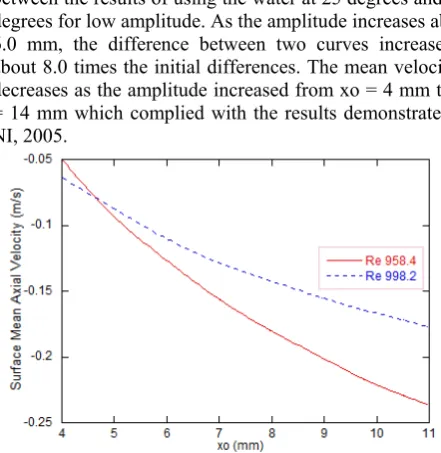
3D simulation was carried out for a total of 80 seconds to investigate the precise details of mixing. The surface Mean average axial velocity calculated by appointing three points in the middle of the geometry and divided to the number of points. The figure 4 shows the mean average velocity versus fluid density for a fixed frequency of 1.0 Hz and a range of amplitudes between 4 mm, 8 mm and 14 mm.
It is clear that there are no significant differences between the results of using the water at 25 degrees and 100 degrees for low amplitude. As the amplitude increases above 6.0 mm, the difference between two curves increases to about 8.0 times the initial differences. The mean velocity is decreases as the amplitude increased from xo = 4 mm to xo = 14 mm which complied with the results demonstrated by NI, 2005.
[image:2.595.49.274.529.600.2]
The mixing was evaluated using an additional variable (AV). The AV can express as a transport equation that is transported through the fluid [8] with the same velocity as the flow. Initially, the AV is described by assigning an expression code in the physics of the simulation, and it tends to divide the domain into two coloured sections to exhibit the process of mixing in the column. Gradually, AV transported through the domain by fluid oscillation and mixes entirely. The average of absolute value of the deviation of AV can be calculated using the function calculator in CFD-Post and then subtracted from 1.0 to calculate the amount of the mixing by the following expression:
M = 1 – Mean value of absolute (Average deviation of AV).
The figure 5 illustrates the variation of amplitude with mixing.
[image:3.595.305.548.54.195.2]
Figure 5 – Fluid mixing versus water density, f= 1 Hz, Xo = 4 mm and 5.7 mm.
The fluid density for water at 25o and 100o plotted for three different oscillation amplitudes of 4 mm, 8 mm and 14 mm with a constant frequency of 1 Hz. It seems that at an amplitude of 4 mm the amount of mixing is higher for the water at room temperature (25 degrees) and there’s a sharp increase in the mixing curve from xo = 4 mm to xo = 8 mm. The curve then increases at a decreasing rate from xo = 8 mm for both densities. The results demonstrated the similar value for both densities at amplitudes of 14 mm.
[image:3.595.48.280.265.411.2]The result demonstrates that the mixing suffer if the water at 100 degrees used at low amplitudes, but it will produce the similar mixing value at high amplitudes. The fluid stream lines are plotted for variation of AV and presented in the figure 5.
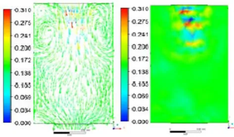
Figure 6 – Comparison of AV streamline maps on a plane of z = 0 at phased one to twelve.
Figure 6 shows the streamlines plotted for variation of AV for a full cycle. At the start of the oscillation cycle (phase one), the AV is at its initial set up mode, i.e., half of the column red and the other blue (as was described earlier). As the flow cycle begins, the flow accelerates and vortex rings form downstream of the orifice baffles. On the other hand, when flow decelerates the previously formed vortices swept into the flow, and new vortices form upstream of the baffle column. The AV can express as a transport equation that is transported through the fluid with the same velocity as the flow. Initially, the AV is described by assigning an expression code in the physics of the simulation, and it tends to divide the domain into two coloured sections to exhibit the process of mixing in the column. Gradually, AV transported through the domain by fluid oscillation and mixes entirely.
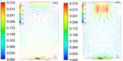
The figure 7 illustrates the variation of velocity vectors with simulation time. The flow is more chaotic for the flow with higher density (at left), which is in conformance with the nature of dimensionless parameter Reynolds number.
[image:3.595.307.547.508.627.2]
Figure 8 – AV contour maps for a simulation at 2.0 s and 29.0 s.
The contour maps of additional variable AV plotted above. The contour maps are able to provide information about the magnitude and amount of AV concentration in the domain.
The AV variation at 2.0 s is between 8.595e-005 kg/m^3 8.419e-001 kg/m^3; indicating a high deviation and low-mixing value, whereas, this variation at 29.0 s is between 1.125e-001 kg/m^3 and 1.489e-001, indicating a low deviation and a high-mixing value.
This information can provide insight and details of the flow behaviour. It appears as the volume average of the AV concentration decreases in the column, the amount of mixing increases. Therefore, as the average volume fraction of AV reduces to 0.0 the full mixing can achieve.
It is apparent that the variation in radial velocity continues throughout the progression of the simulation for both densities. It appears that the radial velocity increases sharply at amplitude of 8 mm. It’s interesting to know that the radial velocity remains almost the same for amplitude of 14 mm when it compares to amplitude of 4 mm. The high oscillatory amplitude of 8 mm promotes a uniform mixing throughout the column.
On the other hand the variation for both fluid densities are similar, with larger variation at xo = 14 mm.
The contours and vectors, plotted for residual of AV for three values of Reynolds numbers between 1257, 2500 and 4525.2. This range of Reynolds numbers presents a laminar, transition and turbulent regimes. The figures at xo = 4 mm show a residual of 0.00005%; whereas, the residuals for xo = 8 mm and xo = 14 mm are around 0.000025% and 0.0000001% respectively, indicating that residuals values decrease faster at higher Reynolds number.
[image:4.595.304.534.70.277.2]
Figure 9 – Variation of AV at different oscillation amplitude at fluid domain, = 998.2 kg/m^3.
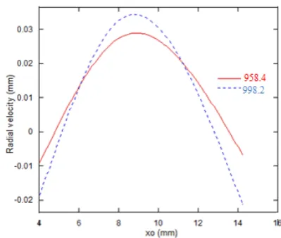
The radial velocity was plotted against the water density for each amplitude and the results are presented below for comparison.
Figure 10 – The variation of amplitude against radial velocity for water densities of 998.2 kg/m^3 and 958.4 kg/m^3.
[image:4.595.326.526.347.516.2] [image:4.595.316.532.559.675.2]
Figure 12 – The vector and contour variable for AV using normalized
symbols at 5.0 s and xo = 8 mm.
Figure 13 – The vector and contour variables for AV using normalized symbols at 5.0 s for xo = 14 mm.
V CONCLUSION
3D numerical method utilised to study the effect of density variation in oscillatory baffled columns (OBCs).
An additional variable AV was introduced as a tracer in CFX-pre software by assigning an expression. The volume average of concentration of this tracer calculated in CFX-post and the mixing parameter M computed based on the assumption that the total volume in the column is equals to 1.0.
This parameter was able to describe the physics behind the mixing by providing the visuals of vectors, streamlines and contours. This approach was performed for the first time resulting in more accurate and precise way of evaluating and estimating of the mixing. Furthermore, the use of this method provides an opportunity for further investigation of factors affecting the mixing and ways to enhance and control the elements that have a significant contribution on mixing.
It also found out that the residuals of AV decreased at higher Reynolds numbers.
It observed that the water at 100o that exhibits a lower density has reversed effect on mixing.
REFERENCE
[1] Ni, X., H. Jian, and A.W. Fitch, Computational fluid dynamic modelling of flow patterns in an
oscillatory baffled column. Chemical
Engineering Science, 2002. 57(14): p.
2849-2862.
[2] Ni, X., et al., Mixing Through Oscillations and Pulsations—A Guide to Achieving Process Enhancements in the Chemical and Process Industries. Chemical Engineering Research and Design, 2003. 81(3): p. 373-383.
[3] Hamzah, A.A., et al., Effect of oscillation amplitude on velocity distributions in an oscillatory baffled column (OBC). Chemical Engineering Research and Design, 2012.
90(8): p. 1038-1044.
[4] Fitch, A.W.J., Hongbing,Ni, Xiongwei, An investigation of the effect of viscosity on mixing in an oscillatory baffled column using digital particle image velocimetry and computational fluid dynamics simulation. Chemical Engineering Journal, 2005. 112(1–
3): p. 197-210.
[5] Johnstone & Yu, Model Development of Single Phase Flow in Oscillatory Baffled Columns Chemica conference, 2013.
[6] Brunold, C.R., et al., Experimental observations on flow patterns and energy losses for oscillatory flow in ducts containing sharp edges. Chemical Engineering Science, 1989. 44(5): p. 1227-1244.
[7] Ni, X. and P. Gough, On the discussion of the dimensionless groups governing oscillatory flow in a baffled tube. Chemical Engineering Science, 1997. 52(18): p. 3209-3212.
[image:5.595.51.288.238.377.2]