Open Domain Targeted Sentiment Analysis via Span Based Extraction and Classification

537

Open-Domain Targeted Sentiment Analysis

via Span-Based Extraction and Classification

Minghao Hu†_{, Yuxing Peng}†_{, Zhen Huang}†_{, Dongsheng Li}†_{, Yiwei Lv}§ †_{National University of Defense Technology, Changsha, China}

§_{University of Macau, Macau, China}

{huminghao09,pengyuxing,huangzhen,dsli}@nudt.edu.cn

Abstract

Open-domain targeted sentiment analysis aims to detect opinion targets along with their senti-ment polarities from a sentence. Prior work typically formulates this task as a sequence tagging problem. However, such formulation suffers from problems such as huge search space and sentiment inconsistency. To ad-dress these problems, we propose a span-based extract-then-classify framework, where multi-ple opinion targets are directly extracted from the sentence under the supervision of target span boundaries, and corresponding polarities are then classified using their span representa-tions. We further investigate three approaches under this framework, namely the pipeline, joint, and collapsed models. Experiments on three benchmark datasets show that our ap-proach consistently outperforms the sequence tagging baseline. Moreover, we find that the pipeline model achieves the best performance compared with the other two models.

1 Introduction

Open-domain targeted sentiment analysis is a fun-damental task in opinion mining and sentiment analysis (Pang et al., 2008; Liu, 2012). Com-pared to traditional sentence-level sentiment anal-ysis tasks (Lin and He,2009;Kim,2014), the task requires detecting target entities mentioned in the sentence along with their sentiment polarities, thus being more challenging. Taking Figure1as an ex-ample, the goal is to first identify “Windows 7” and “Vista” as opinion targets and then predict their corresponding sentiment classes.

Sentence: I love[Windows 7]+which is a vast

improv-ment over[Vista]-. Targets:Windows 7, Vista

Polarities:positive, negative

Figure 1: Open-domain targeted sentiment analysis.

Typically, the whole task can be decoupled into two subtasks. Since opinion targets are not given, we need to first detect the targets from the in-put text. This subtask, which is usually denoted as target extraction, can be solved by sequence tagging methods (Jakob and Gurevych,2010;Liu et al.,2015;Wang et al.,2016a;Poria et al.,2016; Shu et al.,2017;He et al.,2017;Xu et al.,2018). Next, polarity classification aims to predict the sentiment polarities over the extracted target en-tities (Jiang et al., 2011;Dong et al., 2014;Tang et al.,2016a;Wang et al.,2016b;Chen et al.,2017; Xue and Li,2018;Li et al.,2018;Fan et al.,2018). Although lots of efforts have been made to design sophisticated classifiers for this subtask, they all assume that the targets are already given.

Rather than using separate models for each sub-task, some works attempt to solve the task in a more integrated way, by jointly extracting targets and predicting their sentiments (Mitchell et al., 2013; Zhang et al., 2015; Li et al., 2019). The key insight is to label each word with a set of tar-get tags (e.g.,B, I, O) as well as a set of polarity

tags (e.g., +, -, 0), or use a more collapsed set of tags (e.g., B+, I-) to directly indicate the

bound-ary of targeted sentiment, as shown in Figure2(a). As a result, the entire task is formulated as a se-quence tagging problem, and solved using either a pipeline model, a joint model, or a collapsed model under the same network architecture.

Sentence:

Pipeline/ Joint:

I love Windows 7 ... over Vista . O O B I O B O

0 0 + + 0 - 0

Collapsed: O O B+ I+ O B- O

(a) Sequence tagging. The B/I/O labels indicate target span boundaries, while +/-/0 refer to sentiment polarities.

Sentence:

Pipeline/ Joint:

I love Windows 7 ... over Vista .

Target start: 3, 11 Target end: 4, 11

Collapsed:

Polarity: +,

-Target start: 3+, 11- Target end: 4+, 11

-(b) Span-based labeling. The number denotes the start/end position of the given target in the sentence.

Figure 2: Comparison of different annotation schemes for the pipeline, joint, and collapsed models.

ignores the semantics of the entire opinion get. Second, since predicted polarities over tar-get words may be different, the sentiment consis-tency of multi-word entity can not be guaranteed, as mentioned by Li et al. (2019). For example, there is a chance that the words “Windows” and “7” in Figure 2(a)are predicted to have different polarities due to word-level tagging decisions.

To address the problems, we propose a span-based labeling scheme for open-domain targeted sentiment analysis, as shown in Figure2(b). The key insight is to annotate each opinion target with its span boundary followed by its sentiment po-larity. Under such annotation, we introduce an extract-then-classify framework that first extracts multiple opinion targets using an heuristic multi-span decoding algorithm, and then classifies their polarities with corresponding summarized span representations. The advantage of this approach is that the extractive search space can be reduced linearly with the sentence length, which is far less than the tagging method. Moreover, since the po-larity is decided using the targeted span represen-tation, the model is able to take all target words into account before making predictions, thus natu-rally avoiding sentiment inconsistency.

We take BERT (Devlin et al., 2018) as the default backbone network, and explore two re-search questions. First, we make an elaborate comparison between tagging-based models and span-based models. Second, following previous works (Mitchell et al.,2013;Zhang et al.,2015), we compare the pipeline, joint, and collapsed models under the span-based labeling scheme. Ex-tensive experiments on three benchmark datasets show that our models consistently outperform se-quence tagging baselines. In addition, the pipeline model firmly improves over both the joint and col-lapsed models. Source code is released to facilitate future research in this field1_.

1_{https://github.com/huminghao16/SpanABSA}

2 Related Work

Apart from sentence-level sentiment analysis (Lin and He, 2009; Kim, 2014), targeted sentiment analysis, which requires the detection of senti-ments towards mentioned entities in the open do-main, is also an important research topic.

As discussed in §1, this task is usually

di-vided into two subtasks. The first is target ex-traction for identifying entities from the input sen-tence. Traditionally, Conditional Random Fields (CRF) (Lafferty et al.,2001) have been widely ex-plored (Jakob and Gurevych, 2010; Wang et al., 2016a;Shu et al., 2017). Recently, many works concentrate on leveraging deep neural networks to tackle this task, e.g., using CNNs (Poria et al., 2016; Xu et al., 2018), RNNs (Liu et al., 2015; He et al., 2017), and so on. The second is po-larity classification, assuming that the target en-tities are given. Recent works mainly focus on capturing the interaction between the target and the sentence, by utilizing various neural architec-tures such as LSTMs (Hochreiter and Schmidhu-ber,1997;Tang et al.,2016a) with attention mech-anism (Wang et al., 2016b; Li et al., 2018; Fan et al.,2018), CNNs (Xue and Li,2018;Huang and Carley,2018), and Memory Networks (Tang et al., 2016b;Chen et al.,2017;Li and Lam,2017).

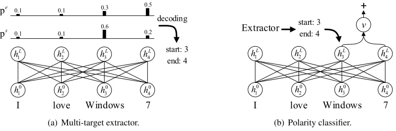
ps

love Windows 7

0 1

h 0

2

h 0

3

h 0

4 h

4L h 3

L h 2L

h 1L

h

0.1 0.1

0.6

0.2

0.1 0.1 0.3 0.5

I

decoding

start: 3 end: 4

pe

(a) Multi-target extractor.

4L

h

3L

h

0 1

h 0

2

h 0

3

h 0

4

h

2L

h

1L

h

+

love Windows 7 I

start: 3 end: 4 Extractor

(b) Polarity classifier.

Figure 3: An overview of the proposed framework. Word embeddings are fed to the BERT encoder (Devlin et al.,

2018) that containsLpre-trained Transformer blocks (Vaswani et al.,2017). The last block’s hidden states are

used to (a) propose one or multiple candidate targets based on the probabilities of the start and end positions, (b) predict the sentiment polarity using the span representation of the given target.

word detection. Our work differs from these ap-proaches in that we formulate this task as a span-level extract-then-classify process instead.

The proposed span-based labeling scheme is in-spired by recent advances in machine comprehen-sion and question answering (Seo et al.,2017;Hu et al., 2018), where the task is to extract a con-tinuous span of text from the document as the an-swer to the question (Rajpurkar et al.,2016). To solve this task, Lee et al.(2016) investigate sev-eral predicting strategies, such as BIO prediction, boundary prediction, and the results show that pre-dicting the two endpoints of the answer is more beneficial than the tagging method. Wang and Jiang(2017) explore two answer prediction meth-ods, namely the sequence method and the bound-ary method, finding that the later performs better. Our approach is related to this line of work. How-ever, unlike these works that extract one span as the final answer, our approach is designed to dy-namically output one or multiple opinion targets.

3 Extract-then-Classify Framework

Instead of formulating the open-domain targeted sentiment analysis task as a sequence tagging problem, we propose to use a span-based label-ing scheme as follows: given an input sentence

x = (x1, ..., xn) with lengthn, and a target list

T = _{t1, ...,tm}, where the number of targets is mand each targettiis annotated with its start po-sition, its end popo-sition, and its sentiment polarity. The goal is to find all targets from the sentence as well as predict their polarities.

The overall illustration of the proposed frame-work is shown in Figure3. The basis of our

frame-work is the BERT encoder (Devlin et al., 2018): we map word embeddings into contextualized to-ken representations using pre-trained Transformer blocks (Vaswani et al., 2017) (§3.1). A multi-target extractor is first used to propose multiple candidate targets from the sentence (§3.2). Then,

a polarity classifier is designed to predict the sen-timent towards each extracted candidate using its summarized span representation (§3.3). We

fur-ther investigate three different approaches under this framework, namely the pipeline, joint, and collapsed models in§3.4.

3.1 BERT as Backbone Network

We use Bidirectional Encoder Representations from Transformers (BERT) (Devlin et al.,2018), a pre-trained bidirectional Transformer encoder that achieves state-of-the-art performances across a va-riety of NLP tasks, as our backbone network.

We first tokenize the sentencexusing a 30,522

wordpiece vocabulary, and then generate the in-put sequence˜xby concatenating a[CLS]token, the tokenized sentence, and a[SEP]token. Then for each tokenx˜i in˜x, we convert it into vector space by summing the token, segment, and posi-tion embeddings, thus yielding the input embed-dingsh0_2R(n+2)⇥h_{, wherehis the hidden size.}

Next, we use a series ofLstacked Transformer blocks to project the input embeddings into a se-quence of contextual vectors hi _{2 R}(n+2)⇥h _as:

hi = TransformerBlock(hi 1),₈i₂[1, L]

3.2 Multi-Target Extractor

Multi-target extractor aims to propose multiple candidate opinion targets (Figure 3(a)). Rather than finding targets via sequence tagging methods, we detect candidate targets by predicting the start and end positions of the target in the sentence, as suggested in extractive question answering (Wang and Jiang,2017;Seo et al.,2017;Hu et al.,2018). We obtain the unnormalized score as well as the probability distribution of the start position as:

gs=wshL, ps= softmax(gs)

wherews2Rhis a trainable weight vector. Simi-larly, we can get the probability of the end position along with its confidence score by:

ge=wehL, pe= softmax(ge)

During training, since each sentence may con-tain multiple targets, we label the span boundaries for all target entities in the listT. As a result, we

can obtain a vectorys _{2 R}(n+2)_{, where each}

el-ementys_i indicates whether thei-th token starts a

target, and also get another vector ye ₂ R(n+2)

for labeling the end positions. Then, we define the training objective as the sum of the negative log probabilities of the true start and end positions on two predicted probabilities as:

L= Xn+2

i=1 y

s

i log(psi)

Xn+2

j=1 y

e

jlog(pej)

At inference time, previous works choose the span (k, l) (k  l) with the maximum value of

g_ks+g_leas the final prediction. However, such

de-coding method is not suitable for the multi-target extraction task. Moreover, simply taking top-K spans according to the addition of two scores is also not optimal, as multiple candidates may re-fer to the same text. Figure 4 gives a qualitative example to illustrate this phenomenon.

Sentence:Great food but the service was dreadful!

Targets:food, service

Predictions: food but the service, food, Great food, ser-vice, service was dreadful, ...

Figure 4: An example shows that there are many re-dundant spans in top-Kpredictions.

To adapt to multi-target scenarios, we pro-pose an heuristic multi-span decoding algorithm as shown in Algorithm1. For each example, top-M indices are first chosen from the two predicted

scoresgs andge (line 2), and the candidate span

(si,ej) (denoted as rl) along with its heuristic-regularized scoreulare then added to the listsR andU respectively, under the constraints that the

end position is no less than the start position as well as the addition of two scores exceeds a thresh-old (line 3-8). Note that we heuristically calcu-lateul as the sum of two scores minus the span length (line 6), which turns out to be critical to the performance as targets are usually short enti-ties. Next, we prune redundant spans inR using

the non-maximum suppression algorithm (Rosen-feld and Thurston,1971). Specifically, we remove the spanrl that possesses the maximum scoreul from the setR and add it to the set O (line

10-11). We also delete any spanrkthat is overlapped withrl, which is measured with the word-level F1

function (line 12-14). This process is repeated for remaining spans inR, untilRis empty or top-K target spans have been proposed (line 9).

Algorithm 1Heuristic multi-span decoding

Input:gs_,ge_{, ,K}

gs_{denotes the score of start positions}

ge_{denotes the score of end positions}

is a minimum score threshold

Kis the maximum number of proposed targets 1: InitializeR,U,O={},{},{}

2: Get top-MindicesS,Efromgs,ge

3: forsiinSdo

4: forejinEdo

5: ifsiejandgssi+g

e

ej then

6: ul=gssi+g

e

ej (ej si+ 1)

7: rl= (si,ej)

8: R=R_[{rl},U=U[{ul}

9: whileR₆=_{}andsize(O)< Kdo

10: l= arg maxU

11: O=O_[{rl};R=R {rl};U=U {ul}

12: forrkinRdo

13: iff1(rl,rk)6= 0then

14: R=R _{rk};U=U {uk}

15: returnO

3.3 Polarity Classifier

Typically, polarity classification is solved using either sequence tagging methods or sophisticated neural networks that separately encode the target and the sentence. Instead, we propose to sum-marize the target representation from contextual sentence vectors according to its span boundary, and use feed-forward neural networks to predict the sentiment polarity, as shown in Figure3(b).

Specifically, given a target spanr, we calculate a summarized vectorvusing the attention

corrsponding bound(si,ej), similar toLee et al. (2017) andHe et al.(2018):

↵= softmax(w↵hLsi:ej)

v=Xej

t=si

↵t si+1h

L t

wherew↵2Rhis a trainable weight vector.

The polarity score is obtained by applying two linear transformations with a Tanh activation in between, and is normalized with the softmax func-tion to output the polarity probability as:

gp =Wptanh(Wvv), pp = softmax(gp)

where Wv 2 Rh⇥h and Wp 2 Rk⇥h are two trainable parameter matrices.

We minimize the negative log probabilities of the true polarity on the predicted probability as:

J = Xk

i=1y

p i log(p

p i)

where yp is an one-hot label indicating the true

polarity, andkis the number of sentiment classes. During inference, the polarity probability is cal-culated for each candidate target span in the setO,

and the sentiment class that possesses the maxi-mum value inpp_{is chosen.}

3.4 Model Variants

Following Mitchell et al. (2013); Zhang et al. (2015), we investigate three kinds of models un-der the extract-then-classify framework:

Pipeline model We first build a multi-target ex-tractor where a BERT encoder is exclusively used. Then, a second backbone network is used to pro-vide contextual sentence vectors for the polarity classifier. Two models are separately trained and combined as a pipeline during inference.

Joint model In this model, each sentence is fed into a shared BERT backbone network that finally branches into two sibling output layers: one for proposing multiple candidate targets and another for predicting the sentiment polarity over each ex-tracted target. A joint training lossL+J is used to optimize the whole model. The inference pro-cedure is the same as the pipeline model.

Collapsed model We combine target span boundaries and sentiment polarities into one label space. For example, the sentence in Figure 2(b) has a positive span (3+,4+) and a negative span

Dataset #Sent #Targets #+ #- #0

LAPTOP 1,869 2,936 1,326 990 620

REST 3,900 6,603 4,134 1,538 931

TWITTER 2,350 3,243 703 274 2,266

Table 1: Dataset statistics. ‘#Sent’ and ‘#Targets’ de-note the number of sentences and targets, respectively. ‘+’, ‘-’, and ‘0’ refer to the positive, negative, and neu-tral sentiment classes.

(11-,11-). We then modify the multi-target

ex-tractor by producing three sets of probabilities of the start and end positions, where each set corre-sponds to one sentiment class ( e.g.,ps+andpe+

for positive targets). Then, we define three objec-tives to optimize towards each polarity. During inference, the heuristic multi-span decoding algo-rithm is performed on each set of scores (e.g.,gs+

andge+_{), and the output setsO}+_{,O , andO}0_are

aggregated as the final prediction.

4 Experiments 4.1 Setup

Datasets We conduct experiments on three benchmark sentiment analysis datasets, as shown in Table 1. LAPTOP contains product reviews from the laptop domain in SemEval 2014 ABSA challenges (Pontiki et al., 2014). REST is the union set of the restaurant domain from SemEval 2014, 2015 and 2016 (Pontiki et al.,2015,2016).

TWITTERis built byMitchell et al.(2013), con-sisting of twitter posts. Following Zhang et al. (2015); Li et al. (2019), we report the ten-fold cross validation results forTWITTER, as there is no train-test split. For each dataset, the gold tar-get span boundaries are available, and the tartar-gets are labeled with three sentiment polarities, namely

positive(+),negative(-), andneutral(0).

Metrices We adopt the precision (P), recall (R), and F1 score as evaluation metrics. A predicted target is correct only if it exactly matches the gold target entity and the corresponding polarity. To separately analyze the performance of two sub-tasks, precision, recall, and F1 are also used for the target extraction subtask, while the accuracy (ACC) metric is applied to polarity classification.

Model settings We use the publicly available BERTLARGE2 model as our backbone network,

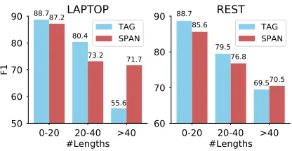
Model _Prec. LAPTOP_{Rec. F1 Prec.} REST_{Rec. F1 Prec.}TWITTER_{Rec. F1}

UNIFIED 61.27 54.89 57.90 68.64 71.01 69.80 53.08 43.56 48.01 TAG-pipeline 65.84 67.19 66.51 71.66 76.45 73.98 54.24 54.37 54.26 TAG-joint 65.43 66.56 65.99 71.47 75.62 73.49 54.18 54.29 54.20 TAG-collapsed 63.71 66.83 65.23 71.05 75.84 73.35 54.05 54.25 54.12 SPAN-pipeline 69.46 66.72 68.06 76.14 73.74 74.92 60.72 55.02 57.69

SPAN-joint 67.41 61.99 64.59 72.32 72.61 72.47 57.03 52.69 54.55 SPAN-collapsed 50.08 47.32 48.66 63.63 53.04 57.85 51.89 45.05 48.11

Table 2: Main results on three benchmark datasets. A BERTLARGEbackbone network is used for both the “TAG”

and “SPAN” models. State-of-the-art results are marked inbold.

and refer readers to Devlin et al. (2018) for de-tails on model sizes. We use Adam optimizer with a learning rate of 2e-5 and warmup over the first 10% steps to train for 3 epochs. The batch size is 32 and a dropout probability of 0.1 is used. The number of candidate spansM is set as 20 while the maximum number of proposed targetsKis 10 (Algorithm1). The threshold is manually tuned on each dataset. All experiments are conducted on a single NVIDIA P100 GPU card.

4.2 Baseline Methods

We compare the proposed span-based approach with the following methods:

TAG-{pipeline, joint, collapsed} are the se-quence tagging baselines that involve a BERT en-coder and a CRF deen-coder. “pipeline” and “joint” denote the pipeline and joint approaches that uti-lize the BIO and +/-/0 tagging schemes, while “collapsed” is the model following the collapsed tagging scheme (Figure2(a)).

UNIFIED (Li et al., 2019) is the current state-of-the-art model on targeted sentiment analysis3_.

It contains two stacked recurrent neural networks enhanced with multi-task learning and adopts the collapsed tagging scheme.

We also compare our multi-target extractor with the following method:

DE-CNN (Xu et al., 2018) is the current state-of-the-art model on target extraction, which com-bines a double embeddings mechanism with con-volutional neural networks (CNNs)4_.

Finally, the polarity classifier is compared with the following methods:

3_{https://github.com/lixin4ever/E2E-TBSA} 4_{https://www.cs.uic.edu/hxu/}

MGAN(Fan et al.,2018) uses a multi-grained at-tention mechanism to capture interactions between targets and sentences for polarity classification.

TNet(Li et al.,2018) is the current state-of-the-art model on polarity classification, which consists of a multi-layer context-preserving network architec-ture and uses CNNs as feaarchitec-ture extractor5_.

4.3 Main Results

We compare models under either the sequence tag-ging scheme or the span-based labeling scheme, and show the results in Table2. We denote our ap-proach as “SPAN”, and use BERTLARGE as back-bone networks for both the “TAG” and “SPAN” models to make the comparison fair.

Two main observations can be obtained from the Table. First, despite that the “TAG” base-lines already outperform previous best approach (“UNIFIED”), they are all beaten by the “SPAN” methods. The best span-based method achieves 1.55%, 0.94% and 3.43% absolute gains on three datasets compared to the best tagging method, in-dicating the efficacy of our extract-then-classify framework. Second, among the span-based meth-ods, the SPAN-pipeline achieves the best perfor-mance, which is similar to the results ofMitchell et al. (2013); Zhang et al.(2015). This suggests that there is only a weak connection between tar-get extraction and polarity classification. The con-clusion is also supported by the result of SPAN-collapsed method, which severely drops across all datasets, implying that merging polarity labels into target spans does not address the task effectively.

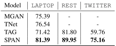
Model LAPTOP REST TWITTER

DE-CNN 81.59 -

-TAG 85.20 84.48 73.47

SPAN 83.35 82.38 75.28

Table 3: F1 comparison of different approaches for target extraction.

Figure 5: F1 onLAPTOPandRESTw.r.t different sen-tence lengths for target extraction.

4.4 Analysis on Target Extraction

To analyze the performance on target extraction, we run both the tagging baseline and the multi-target extractor on three datasets, as shown in Ta-ble 3. We find that the BIO tagger outperforms our extractor onLAPTOPandREST. A likely rea-son for this observation is that the lengths of input sentences on these datasets are usually small (e.g., 98% of sentences are less than 40 words inREST), which limits the tagger’s search space (the power set of all sentence words). As a result, the com-putational complexity has been largely reduced, which is beneficial for the tagging method.

In order to confirm the above hypothesis, we plot the F1 score with respect to different sen-tence lengths in Figure 5. We observe that the performance of BIO tagger dramatically decreases as the sentence length increases, while our tor is more robust for long sentences. Our extrac-tor manages to surpass the tagger by 16.1 F1 and 1.0 F1 when the length exceeds 40 on LAPTOP

andREST, respectively. The above result demon-strates that our extractor is more suitable for long sentences due to the fact that its search space only increases linearly with the sentence length.

Since a trade-off between precision and recall can be adjusted according to the threshold in our extractor, we further plot the precision-recall curves under different ablations to show the ef-fects of heuristic multi-span decoding algorithm. As can be seen from Figure6, ablating the length

Figure 6: Precision-recall curves on LAPTOP and

RESTfor target extraction. “NMS” and “heuristics” denote the non-maximum suppression and the length heuristics in Algorithm1.

heuristics results in consistent performance drops across two datasets. By sampling incorrect predic-tions we find that there are many targets closely aligned with each other, such as “perfect [size]+ and [speed]+”, “[portions]+ all at a reasonable [price]+”, and so on. The model without length heuristics is very likely to output the whole phrase as a single target, thus being totally wrong. More-over, removing the non-maximum suppression (NMS) leads to significant performance degrada-tions, suggesting that it is crucial to prune redun-dant spans that refer to the same text.

4.5 Analysis on Polarity Classification

To assess the polarity classification subtask, we compare the performance of our span-level polar-ity classifier with the CRF-based tagger in Table 5. The results show that our approach signifi-cantly outperforms the tagging baseline by achiev-ing 9.97%, 8.15% and 15.4% absolute gains on three datasets, and firmly surpasses previous state-of-the-art models onLAPTOP. The large improve-ment over the tagging baseline suggests that de-tecting sentiment with the entire span representa-tion is much more beneficial than predicting polar-ities over each word, as the semantics of the given target has been fully considered.

Sentence TAG SPAN 1. I thought the transition would be difficult at best and would take some time

to fully familiarize myself with the new[Mac ecosystem]0. [ecosystem]+(7) [Mac ecosystem]0

2. I would normally not finish the[brocolli]+when I order these kinds of food

but for the first time, every piece was as eventful as the first one... the[scallops]+

and[prawns]+was so fresh and nicely cooked.

[brocolli]-(7),

[scallops and prawns]+(7),

[food]0(7)

[brocolli]+,

[scallops]+,

[prawns]+

3. I like the[brightness]+and[adjustments]+. [brightness]+, [adjustments]+ [brightness]+, None (7)

4. The[waiter]-was a bit unfriendly and the[feel]-of the restaurant was crowded. [waiter]-, [feel]- [waiter]-, None (7)

5. However, it did not have any scratches, zero[battery cycle count]+(pretty

surprised), and all the[hardware]+seemed to be working perfectly.

[battery cycle count]0(7),

[hardware]+

[battery cycle count]+,

[hardware]+

6. I agree that dining at[Casa La Femme]-is like no other dining experience! [Casa La Femme]+(7) [Casa La Femme]

-Table 4: Case study. The extracted targets are wrapped in brackets with the predicted polarities given as subscripts. Incorrect predictions are marked with7_.

Model LAPTOP REST TWITTER

MGAN 75.39 -

-TNet 76.54 -

-TAG 71.42 81.80 59.76

SPAN 81.39 89.95 75.16

Table 5: Accuracy comparison of different approaches for polarity classification.

span-based method, on the contrary, can naturally alleviate such problem because the polarity is clas-sified by taking all target words into account.

4.6 Case Study

Table 4 shows some qualitative cases sampled from the pipeline methods. As observed in the first two examples, the “TAG” model incorrectly predicts the target span by either missing the word “Mac” or proposing a phrase across two targets (“scallps and prawns”). A likely reason of its fail-ure is that the input sentences are relatively longer, and the tagging method is less effective when deal-ing with them. But when it comes to shorter in-puts (e.g., the third and the fourth examples), the tagging baseline usually performs better than our approach. We find that our approach may some-times fail to propose target entities (e.g., “ adjust-ments” in (3) and “feel” in (4)), which is due to the fact that a relatively large has been set. As a result, the model only makes cautious but confi-dent predictions. In contrast, the tagging method does not rely on a threshold and is observed to have a higher recall. For example, it additionally predicts the entity “food” as a target in the sec-ond example. Moreover, we find that the tagging method sometimes fails to predict the correct

sen-Figure 7: Accuracy onLAPTOPandRESTw.r.t differ-ent number of target words for polarity classification.

timent class, especially when the target consists of multiple words (e.g., “battery cycle count” in (5) and “Casa La Femme” in (6)), indicating the tag-ger can not effectively maintain sentiment consis-tency across words. Our polarity classifier, how-ever, can avoid such problem by using the target span representation to predict the sentiment.

5 Conclusion

suitable for long sentences. Moreover, we find that the pipeline model consistently surpasses both the joint model and the collapsed model.

Acknowledgments

We thank the anonymous reviewers for their in-sightful feedback. We also thank Li Dong for his helpful comments and suggestions. This work was supported by the National Key Re-search and Development Program of China (2016YFB1000101).

References

Dzmitry Bahdanau, Kyunghyun Cho, and Yoshua Ben-gio. 2014. Neural machine translation by jointly learning to align and translate. arXiv preprint arXiv:1409.0473.

Peng Chen, Zhongqian Sun, Lidong Bing, and Wei Yang. 2017. Recurrent attention network on mem-ory for aspect sentiment analysis. InProceedings of EMNLP.

Jacob Devlin, Ming-Wei Chang, Kenton Lee, and Kristina Toutanova. 2018. Bert: Pre-training of deep bidirectional transformers for language understand-ing. arXiv preprint arXiv:1810.04805.

Li Dong, Furu Wei, Chuanqi Tan, Duyu Tang, Ming Zhou, and Ke Xu. 2014. Adaptive recursive neural network for target-dependent twitter sentiment clas-sification. InProceedings of ACL.

Feifan Fan, Yansong Feng, and Dongyan Zhao. 2018. Multi-grained attention network for aspect-level sentiment classification. InProceedings of EMNLP. Luheng He, Kenton Lee, Omer Levy, and Luke Zettle-moyer. 2018. Jointly predicting predicates and ar-guments in neural semantic role labeling. arXiv preprint arXiv:1805.04787.

Ruidan He, Wee Sun Lee, Hwee Tou Ng, and Daniel Dahlmeier. 2017. An unsupervised neural attention model for aspect extraction. InProceedings of ACL. Sepp Hochreiter and J¨urgen Schmidhuber. 1997. Long

short-term memory.Neural computation.

Minghao Hu, Yuxing Peng, Zhen Huang, Xipeng Qiu, Furu Wei, and Ming Zhou. 2018. Reinforced mnemonic reader for machine reading comprehen-sion. InProceedings of IJCAI.

Binxuan Huang and Kathleen Carley. 2018. Parameter-ized convolutional neural networks for aspect level sentiment classification. InProceedings of EMNLP. Niklas Jakob and Iryna Gurevych. 2010. Extracting opinion targets in a single-and cross-domain setting with conditional random fields. InProceedings of EMNLP.

Long Jiang, Mo Yu, Ming Zhou, Xiaohua Liu, and Tiejun Zhao. 2011. Target-dependent twitter senti-ment classification. InProceedings of ACL.

Yoon Kim. 2014. Convolutional neural networks for sentence classification.

John Lafferty, Andrew McCallum, and Fernando CN Pereira. 2001. Conditional random fields: Prob-abilistic models for segmenting and labeling se-quence data. InProceedings of ICML.

Kenton Lee, Luheng He, Mike Lewis, and Luke Zettle-moyer. 2017. End-to-end neural coreference resolu-tion.arXiv preprint arXiv:1707.07045.

Kenton Lee, Shimi Salant, Tom Kwiatkowski, Ankur Parikh, Dipanjan Das, and Jonathan Berant. 2016. Learning recurrent span representations for ex-tractive question answering. arXiv preprint arXiv:1611.01436.

Xin Li, Lidong Bing, Wai Lam, and Bei Shi. 2018. Transformation networks for target-oriented senti-ment classification. InProceedings of ACL.

Xin Li, Lidong Bing, Piji Li, and Wai Lam. 2019. A unified model for opinion target extraction and target sentiment prediction. InProceedings of AAAI.

Xin Li and Wai Lam. 2017. Deep multi-task learning for aspect term extraction with memory interaction. InProceedings of EMNLP.

Chenghua Lin and Yulan He. 2009. Joint senti-ment/topic model for sentiment analysis. In Pro-ceedings of CIKM.

Bing Liu. 2012. Sentiment analysis and opinion min-ing. Synthesis lectures on human language tech-nologies, 5(1):1–167.

Pengfei Liu, Shafiq Joty, and Helen Meng. 2015. Fine-grained opinion mining with recurrent neural net-works and word embeddings. In Proceedings of EMNLP.

Margaret Mitchell, Jacqui Aguilar, Theresa Wilson, and Benjamin Van Durme. 2013. Open domain tar-geted sentiment. InProceedings of EMNLP.

Bo Pang, Lillian Lee, et al. 2008. Opinion mining and sentiment analysis. Foundations and TrendsR in

In-formation Retrieval, 2(1–2):1–135.

Maria Pontiki, Dimitris Galanis, Haris Papageor-giou, Ion Androutsopoulos, Suresh Manandhar, AL-Smadi Mohammad, Mahmoud Al-Ayyoub, Yanyan Zhao, Bing Qin, Orph´ee De Clercq, et al. 2016. Semeval-2016 task 5: Aspect based sentiment anal-ysis. InProceedings of SemEval-2016.

Maria Pontiki, Dimitris Galanis, John Pavlopoulos, Harris Papageorgiou, Ion Androutsopoulos, and Suresh Manandhar. 2014. Semeval-2014 task 4: As-pect based sentiment analysis. In Proceedings of SemEval-2014.

Soujanya Poria, Erik Cambria, and Alexander Gel-bukh. 2016. Aspect extraction for opinion min-ing with a deep convolutional neural network. Knowledge-Based Systems, 108:42–49.

Pranav Rajpurkar, Jian Zhang, Konstantin Lopyrev, and Percy Liang. 2016. Squad: 100,000+ questions for machine comprehension of text. InProceedings of EMNLP.

Azriel Rosenfeld and Mark Thurston. 1971. Edge and curve detection for visual scene analysis. IEEE Transactions on computers, (5):562–569.

Minjoon Seo, Aniruddha Kembhavi, Ali Farhadi, and Hannaneh Hajishirzi. 2017. Bidirectional attention flow for machine comprehension. InProceedings of ICLR.

Lei Shu, Hu Xu, and Bing Liu. 2017. Lifelong learning crf for supervised aspect extraction. InProceedings of the ACL.

Duyu Tang, Bing Qin, Xiaocheng Feng, and Ting Liu. 2016a. Effective lstms for target-dependent senti-ment classification. InProceedings of COLING. Duyu Tang, Bing Qin, and Ting Liu. 2016b. Aspect

level sentiment classification with deep memory net-work. arXiv preprint arXiv:1605.08900.

Ashish Vaswani, Noam Shazeer, Niki Parmar, Jakob Uszkoreit, Llion Jones, Aidan N Gomez, Łukasz Kaiser, and Illia Polosukhin. 2017. Attention is all you need. InProceedings of NIPS.

Shuohang Wang and Jing Jiang. 2017. Machine com-prehension using match-lstm and answer pointer. In Proceedings of ICLR.

Wenya Wang, Sinno Jialin Pan, Daniel Dahlmeier, and Xiaokui Xiao. 2016a. Recursive neural conditional random fields for aspect-based sentiment analysis. InProceedings of EMNLP.

Yequan Wang, Minlie Huang, Li Zhao, et al. 2016b. Attention-based lstm for aspect-level sentiment clas-sification. InProceedings of EMNLP.

Hu Xu, Bing Liu, Lei Shu, and Philip S Yu. 2018. Dou-ble embeddings and cnn-based sequence labeling for aspect extraction. InProceedings of ACL.

Wei Xue and Tao Li. 2018. Aspect based sentiment analysis with gated convolutional networks. arXiv preprint arXiv:1805.07043.