Interpretable and Compositional Relation Learning by Joint Training with an Autoencoder

2148

Interpretable and Compositional Relation Learning by Joint Training

with an Autoencoder

Ryo Takahashi*1 and Ran Tian*1 and Kentaro Inui1,2 (* equal contribution)

1_{Tohoku University} 2_{RIKEN, Japan}

{ryo.t, tianran, inui}@ecei.tohoku.ac.jp

Abstract

Embedding models for entities and rela-tions are extremely useful for recovering missing facts in a knowledge base. In-tuitively, a relation can be modeled by a matrix mapping entity vectors. How-ever, relations reside on low dimension sub-manifolds in the parameter space of arbitrary matrices – for one reason, com-position of two relations M1,M2 may

match a third M3 (e.g. composition

of relations currency of country

andcountry of filmusually matches

currency of film budget), which imposes compositional constraints to be satisfied by the parameters (i.e.M1·M2≈

M3). In this paper we investigate a

dimen-sion reduction technique by training rela-tions jointly with an autoencoder, which is expected to better capture compositional constraints. We achieve state-of-the-art on Knowledge Base Completion tasks with strongly improved Mean Rank, and show that joint training with an autoencoder leads to interpretable sparse codings of rela-tions, helps discovering compositional con-straints and benefits from compositional training. Our source code is released at github.com/tianran/glimvec.

1 Introduction

Broad-coverage knowledge bases (KBs) such as Freebase (Bollacker et al., 2008) and DBPe-dia (Auer et al.,2007) store a large amount of facts in the form of hhead entity, relation, tail entityi triples (e.g. hThe Matrix, country of film, Australiai), which could support a wide range of reasoning and question answering applications. The Knowledge Base Completion (KBC) task aims

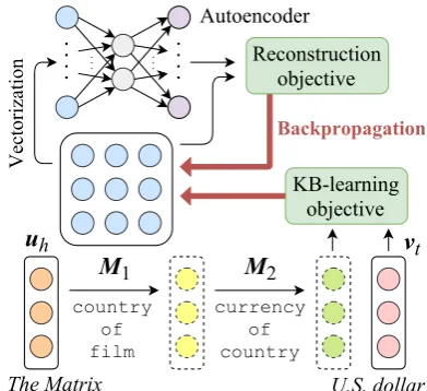
Figure 1: In joint training, relation parameters (e.g. M1) receive updates from both aKB-learning

ob-jective, trying to predict entities in the KB; and a re-construction objectivefrom an autoencoder, trying to recover relations from low dimension codings.

to predict the missing part of an incomplete triple, such ashFinding Nemo,country of film, ?i, by reasoning from known facts stored in the KB.

as mappings from head to tail entities, and the composition of two maps can match a third (e.g. the composition of currency of country

and country of film matches the relation

currency of film budget), which could be captured by modeling composition in a space.

However, modeling relations as mappings natu-rally requires more parameters – a general linear map betweend-dimension vectors is represented by a matrix ofd2parameters – which are less likely to be shared, impeding transfers of facts between sim-ilar relations. Thus, it is desired to reduce dimen-sionality of relations; furthermore, the existence of a composition of two relations (assumed to be mod-eled by matricesM1,M2) matching a third (M3)

also justifies dimension reduction, because it im-plies acompositional constraintM1·M2 ≈M3

that can be satisfied only by a lower dimension sub-manifold in the parameter space1_.

Previous approaches reduce dimensionality of relations by imposing pre-designed hard con-straints on the parameter space, such as constrain-ing that relations are translations (Bordes et al.,

2013) or diagonal matrices (Yang et al., 2015), or assuming they are linear combinations of a small number of prototypes (Xie et al., 2017). However, pre-designed hard constraints do not seem to cope well with compositional constraints, because it is difficult to know a priori which two relations compose to which third relation, hence difficult to choose a pre-design; and com-positional constraints are not always exact (e.g. the composition of currency of country

andheadquarter locationusually matches

business operation currencybut not al-ways), so hard constraints are less suited.

In this paper, we investigate an alternative ap-proach by training relation parameters jointly with an autoencoder (Figure1). During training, the au-toencoder tries to reconstruct relations from low di-mension codings, with the reconstruction objective back-propagating to relation parameters as well. We show this novel technique promotes parame-ter sharing between different relations, and drives them toward low dimension manifolds (Sec.6.2). Besides, we expect the technique to cope better with compositional constraints, because it discov-ers low dimension manifolds posteriorly from data, and it does not impose any explicit hard constraints.

1_{It is noteworthy that similar compositional constraints}

apply to most modeling schemes of relations, not just matrices.

Yet, joint training with an autoencoder is not simple; one has to keep a subtle balance between gradients of the reconstruction and KB-learning objectives throughout the training process. We are not aware of any theoretical principles directly addressing this problem; but we found some im-portant settings after extensive pre-experiments (Sec.4). We evaluate our system using standard KBC datasets, achieving state-of-the-art on several of them (Sec.6.1), with strongly improved Mean Rank. We discuss detailed settings that lead to the performance (Sec.4.1), and we show that joint train-ing with an autoencoder indeed helps discovertrain-ing compositional constraints (Sec.6.2) and benefits from compositional training (Sec.6.3).

2 Base Model

A knowledge base (KB) is a set T of triples of the form hh, r, ti, where h, t ∈ E are enti-ties and r ∈ R is a relation (e.g. hThe Matrix,

country of film,Australiai). A relationrhas its inverser−1∈ Rso that for everyhh, r, ti ∈ T, we regardht, r−1, hias also in the KB. Under this assumption and givenT as training data, we con-sider the Knowledge Base Completion (KBC) task that predicts candidates for a missing tail entity in an incompletehh, r,?itriple.

Most approaches tackle this problem by train-ing ascore functionmeasuring the plausibility of triples being facts. The model we implement in this work represents entitiesh, tas d-dimension vectorsuh,vtrespectively, and relationras ad×d

matrixMr. Ifuh,vtare one-hot vectors with

di-mensiond=|E|corresponding to each entity, one can take Mr as the adjacency matrix of entities

joined by relationr, so the set of tail entities filling into hh, r,?i is calculated by u>_hMr (with each

nonzero entry corresponds to an answer). Thus, we haveu>_hMrvt>0if and only ifhh, r, ti ∈ T.

This motivates us to useu>_hMrvtas a natural

pa-rameter to model plausibility ofhh, r, ti, even in a low dimension space with d |E|. Thus, we define the score function as

s(h, r, t) := exp(u>_hMrvt) (1)

for the basic model. This is similar to the bilinear model ofNickel et al.(2011), except that we distin-guishuh(the vector for head entities) fromvt(the

More generally, we considercompositionof re-lationsr1/ . . . /rl to modelpaths in a KB (Guu

et al.,2015), as defined byr1, . . . , rlparticipating

in a sequence of facts such that the head entity of each fact coincides with the tail of its previous. For example, a sequence of two factshThe Matrix,

country of film, Australiai and hAustralia,

currency of country, Australian Dollari form a path of compositioncountry of film/

currency of country, because the head of the second fact (i.e.Australia) coincides with the tail of the first. Using the previous d = |E| ana-logue, one can verify that composition of relations is represented by multiplication of adjacency ma-trices, so we accordingly define

s(h, r1/ . . . /rl, t) := exp(u>hMr1· · ·Mrlvt)

to measure the plausibility of a path. It is explored inGuu et al.(2015) to learn a score function not only for single facts but also for paths. This compo-sitional trainingscheme is shown to bring valuable information about the structure of the KB and may help KBC. In this work, we conduct experiments both with and without compositional training.

In order to learn parametersuh,vt,Mrof the

score function, we followTian et al.(2016) using a Noise Contrastive Estimation (NCE) (Gutmann and Hyv¨arinen,2012) objective. For each path (or triple)hh, r1/ . . . , titaken from the KB, we

gener-ate negative samples by replacing the tail entityt

with some random noiset∗. Then, we maximize L1 :=

X

path

ln s(h, r1/ . . . , t)

k+s(h, r1/ . . . , t)

+X

noise

ln k

k+s(h, r1/ . . . , t∗)

as ourKB-learning objective. Here,kis the num-ber of noises generated for each path. When the score function is regarded as probability,L1

rep-resents the log-likelihood of “hh, r1/ . . . , tibeing

actual path andhh, r1/ . . . , t∗ibeing noise”.

Max-imizingL1 increases the scores of actual paths and

decreases the scores of noises.

3 Joint Training with an Autoencoder

Autoencoders learn efficient codings of high-dimensional data while trying to reconstruct the original data from the coding. By joint training relation matrices with an autoencoder, we also ex-pect it to help reducing the dimensionality of the original data (i.e. relation matrices).

Formally, we define avectorizationmrfor each

relation matrixMr, and use it as input to the

au-toencoder.mris defined as a reshape ofMr

flat-tened into ad2-dimension vector, and normalized such thatkmrk=

√

d. We define

cr:= ReLU(Amr) (2)

as the coding. Here A is ac ×d2 matrix with

c d2, and ReLUis the Rectified Linear Unit function (Nair and Hinton,2010). We reconstruct the input fromcrby multiplying ad2×cmatrixB.

We wantBcrto be more similar tomrthan other

relations. For this purpose, we define a similarity

g(r1, r2) := exp(

1 √

dcm

>

r1Bcr2), (3)

which measures the length ofBcr2 projected to the

direction ofmr1. In order to learn the parameters

A,B, we adopt the Noise Contrastive Estimation scheme as in Sec.2, generate random noisesr∗ for each relationrand maximize

L₂:= X

r∈R

ln g(r, r)

k+g(r, r) +

X

r∗_∼R

ln k

k+g(r, r∗₎

as ourreconstruction objective. MaximizingL2

increasesmr’s similarity withBcr, and decreases

it withBcr∗.

During joint training, both L1 and L2 are

si-multaneously maximized, and the gradient ∇L2

propagates to relation matrices as well. Since∇L₂ depends onAandB, andA,B interact with all relations, they promote indirect parameter sharing between different relation matrices. In Sec.6.2, we further show that joint training drives relations to-ward a low dimension manifold.

4 Optimization Tricks

Joint training with an autoencoder is not simple. Relation matrices receive updates from both∇L₁ and∇L2, but if they update∇L1 too much, the

autoencoder has no effect; conversely, if they up-date∇L₂too often, all relation matrices crush into one cluster. Furthermore, an autoencoder should learn from genuine patterns of relation matrices that emerge from fitting the KB, but not the re-verse – in which the autoencoder imposes arbitrary patterns to relation matrices according to random initialization. Therefore, it is not surprising that a naive optimization ofL1+L2does not work.

most important “magic” is the scaling factor √1

dc

in definition of the similarity function (3), perhaps being combined with other settings as we discuss below. We have tried different factors1, √1

d, 1

√

c

and _dc1 instead, with various combinations ofdand

c; but the autoencoder failed to learn meaningful codings in other settings. When the scaling factor is too small (e.g. _dc1), all relations get almost the same coding; conversely if the factor is too large (e.g. 1), all codings get very close to0.

The next important rule is to keep a balance be-tween the updates coming from∇L₁and∇L₂. We use Stochastic Gradient Descent (SGD) for opti-mization, and the common practice (Bottou,2012) is to set the learning rate as

α(τ) := η

1 +ηλτ. (4)

Here,η, λare hyper-parameters andτ is a counter of processed data points. In this work, in order to control the updates in detail to keep a balance, we modify (4) to use a a step counterτr for each

relationr, counting “number of updates” instead of data points2. That is, wheneverMrgets a nonzero

update from a gradient calculation,τrincreases by 1. Furthermore, we use different hyper-parameters for different “types of updates”, namelyη1, λ1 for

updates coming from∇L1, andη2, λ2for updates

coming from ∇L₂. Thus, let ∆1 be the partial

gradient of ∇L1, and ∆2 the partial gradient of

∇L2, we updateMrbyα1(τr)∆1+α2(τr)∆2 at

each step, where

α1(τr) := η1

1 +η1λ1τr

, α2(τr) := η2

1 +η2λ2τr .

The rule for settingη1, λ1andη2, λ2is that,η2

should be much smaller than η1, because η1, η2

control the magnitude of learning rates at the early stage of training, with the autoencoder still largely random and∆2 not making much sense; on the

other hand, one has to chooseλ1andλ2such that

k∆₁k/λ1andk∆2k/λ2are at the same scale,

be-cause the learning rates approach 1/(λ1τr) and

1/(λ2τr)respectively, as the training proceeds. In

this way, the autoencoder will not impose random patterns to relation matrices according to its ini-tialization at the early stage, and a balance is kept betweenα1(τr)∆1andα2(τr)∆2 later.

But how to estimatek∆₁kandk∆₂k? It seems that we can approximately calculate their scales

2_{Similarly, we set separate step counters for all head and}

tail entities, and the autoencoder as well.

from initialization. In this work, we use i.i.d. Gaus-sians of variance1/dto initialize parameters, so the initial Euclidean norms arekuhk ≈ 1,kvtk ≈ 1,

kMrk ≈

√

d, and kBAmrk ≈

√

dc. Thus, by calculating ∇L1 and ∇L2 using (1) and (3), we

have approximately

k∆1k ≈ kuhvt>k ≈1, and

k∆₂k ≈ k√1

dcBcrk ≈

1 √

dckBAmrk ≈1.

It suggests that, because of the scaling factor √1

dc

in (3), we havek∆1kandk∆2kat the same scale,

so we can setλ1 =λ2. This might not be a mere

coincidence.

4.1 Training the Base Model

Besides the tricks for joint training, we also found settings that significantly improve the base model on KBC, as briefly discussed below. In Sec.6.3, we will show performance gains by these settings using the FB15k-237 validation set.

Normalization It is better to normalize relation matrices to kMrk =

√

d during training. This might reduce fluctuations in entity vector updates.

Regularizer It is better to minimizekM_r>Mr− 1

dtr(M

>

r Mr)Ikduring training. This regularizer

drivesMrtoward an orthogonal matrix (Tian et al.,

2016) and might reduce fluctuations in entity vector updates. As a result, all relation matrices trained in this work are very close to orthogonal.

Initialization Instead of pure Gaussian, it is bet-ter to initialize matrices as(I +G)/2, whereG

is random. The identity matrix I helps passing information from head to tail (Tian et al.,2016).

Negative Sampling Instead of a unigram distri-bution, it is better to use a uniform distribution for generating noises. This is somehow counter-intuitive compared to training word embeddings.

5 Related Works

KBs have a wide range of applications (Berant et al.,2013;Hixon et al.,2015;Nickel et al.,2016a) and KBC has inspired a huge amount of research (Bordes et al.,2013;Riedel et al., 2013;Socher et al.,2013;Wang et al.,2014b,a;Xiao et al.,2016;

Among the previous works, TransE (Bordes et al., 2013) is the classic method which repre-sents a relation as a translation of the entity vector space, and is partially inspired byMikolov et al.

(2013)’s vector arithmetic method of solving word analogy tasks. Although competitive in KBC, it is speculated that this method is well-suited for1 -to-1relations but might be too simple to represent

N-to-N relations accurately(Wang et al., 2017). Thus, extensions such as TransR (Lin et al.,2015b) and STransE (Nguyen et al.,2016) are proposed to map entities into a relation-specific vector space before translation. The ITransF model (Xie et al.,

2017) further enhances this approach by imposing a hard constraint that the relation-specific maps should be linear combinations of a small number of prototypical matrices. Our work inherits the same motivation with ITransF in terms of promot-ing parameter-sharpromot-ing among relations.

On the other hand, the base model used in this work originates from RESCAL (Nickel et al.,

2011), in which relations are naturally represented as analogue to the adjacency matrices (Sec.2). Fur-ther developments include HolE (Nickel et al.,

2016b) and ConvE (Dettmers et al.,2018) which improve this approach in terms of parameter-efficiency, by introducing low dimension factoriza-tions of the matrices. We inherit the basic model of RESCAL but draw additional training techniques from Tian et al. (2016), and show that the base model already can achieve near state-of-the-art per-formance (Sec.6.1,6.3). This sends a message sim-ilar to Kadlec et al. (2017), saying that training tricks might be as important as model designs.

Nevertheless, we emphasize the novelty of this work in that the previous models mostly achieve di-mension reduction by imposing some pre-designed hard constraints (Bordes et al.,2013;Yang et al.,

2015;Trouillon et al.,2016;Nickel et al.,2016b;

Xie et al.,2017;Dettmers et al.,2018), whereas the constraints themselves are not learned from data; in contrast, our approach by jointly training an autoen-coder does not impose any explicit hard constraints, so it leads to more flexible modeling.

Moreover, we additionally focus on leveraging composition in KBC. Although this idea has been frequently explored before (Guu et al.,2015; Nee-lakantan et al.,2015;Lin et al.,2015a), our discus-sion about the concept of compositional constraints and its connection to dimension reduction has not been addressed similarly in previous research. In

experiments, we will show (Sec.6.2,6.3) that joint training with an autoencoder indeed helps finding compositional constraints and benefits from com-positional training.

Autoencoders have been used solo for learn-ing distributed representations of syntactic trees (Socher et al.,2011), words and images (Silberer and Lapata, 2014), or semantic roles (Titov and Khoddam,2015). It is also used for pretraining other deep neural networks (Erhan et al., 2010). However, when combined with other models, the learning of autoencoders, or more generallysparse codings(Rubinstein et al.,2010), is usually con-veyed in an alternating manner, fixing one part of the model while optimizing the other, such as in

Xie et al.(2017). To our knowledge, joint training with an autoencoder is not widely used previously for reducing dimensionality.

Jointly training an autoencoder is not simple be-cause it takes non-stationary inputs. In this work, we modified SGD so that it shares traits with some modern optimization algorithms such as Adagrad (Duchi et al., 2011), in that they both set differ-ent learning rates for differdiffer-ent parameters. While Adagrad sets them adaptively by keeping track of gradients for all parameters, our modification of SGD is more efficient and allows us to grasp a rough intuition about which parameter gets how much update. We believe our techniques and find-ings in joint training with an autoencoder could be helpful to reducing dimensionality and improving interpretability in other neural network architec-tures as well.

6 Experiments

We evaluate on standard KBC datasets, including WN18 and FB15k (Bordes et al.,2013), WN18RR (Dettmers et al.,2018) and FB15k-237 (Toutanova and Chen, 2015). The statistical information of these datasets are shown in Table1.

Dataset |E| |R| #Train #Valid #Test

WN18 40,943 18 141,442 5,000 5,000 FB15k 14,951 1,345 483,142 50,000 59,071 WN18RR 40,943 11 86,835 3,034 3,134 FB15k-237 14,541 237 272,115 17,535 20,466

Table 1: Statistical information of the KBC datasets. |E|and|R|denote the number of entities and rela-tion types, respectively; #Train, #Valid, and #Test are the numbers of triples in the training, validation, and test sets, respectively.

For all datasets, we set the dimensiond= 256 andc= 16, the SGD hyper-parametersη1= 1/64, η2 = 2−14 and λ1 = λ2 = 2−14. The training

batch size is 32 and the triples in each batch share the same head entity. We compare the base model (BASE) to our joint training with an autoencoder model (JOINT), and the base model with compo-sitional training (BASE+COMP) to our joint model with compositional training (JOINT+COMP). When compositional training is enabled (BASE+COMP, JOINT+COMP), we use random walk to sample paths of length 1 +X, whereX is drawn from a Poisson distribution of meanλ= 1.0.

For any incomplete triplehh, r,?iin KBC test, we calculate a scores(h, r, e)from (1), for every entitye∈ E such thathh, r, eidoes not appear in any of the training, validation, or test sets(Bordes et al.,2013). Then, the calculated scores together with s(h, r, t) for the gold triple is converted to ranks, and the rank of the gold entitytis used for evaluation. Evaluation metrics include Mean Rank (MR), Mean Reciprocal Rank (MRR), and Hits at 10 (H10). Lower MR, higher MRR, and higher H10 indicate better performance.

We consult MR and MRR on validation sets to determine training epochs; we stop training when both MR and MRR have stopped improving.

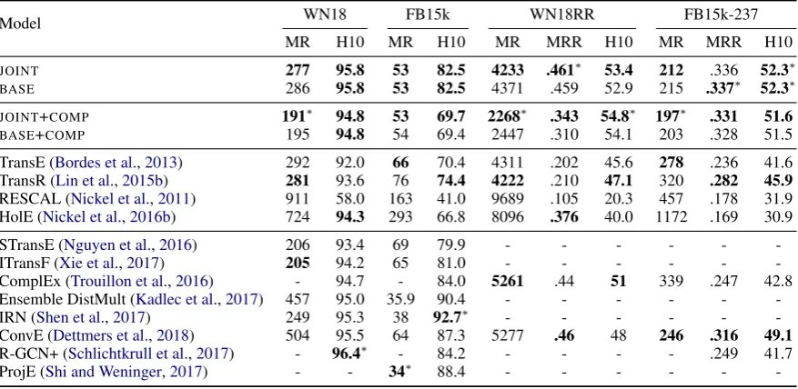
6.1 KBC Results

The results are shown in Table 2. We found that joint training with an autoencoder mostly improves performance, and the improvement be-comes more clear when compositional training is enabled (i.e.,JOINT≥BASEandJOINT+COMP> BASE+COMP). This is convincing because gener-ally, joint training contributes with its regulariz-ing effects, and drastic improvements are less ex-pected3. When compositional training is enabled,

3_{The source code and trained models are publicly released}

athttps://github.com/tianran/glimvec, where

profession profession−1

film_crew_role−1

film_release_region−1

film_language−1

nationality currency_of_country currency_of_company currency_of_university currency_of_film_budget

2 4 6 8 10 12 14 16 currency_of_film_budget

release_region_of_film corporation_of_film producer_of_film writer_of_film

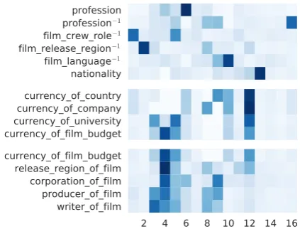
Figure 2: Examples of relation codings learned from FB15k-237. Each row shows a 16 dimension vector encoding a relation. Vectors are normalized such that their entries sum to1.

the system usually achieves better MR, though not always improves in other measures. The perfor-mance gains are more obvious on the WN18RR and FB15k-237 datasets, possibly because WN18 and FB15k contain a lot of easy instances that can be solved by a simple rule (Dettmers et al.,2018). Furthermore, the numbers demonstrated by our joint and base models are among the strongest in the literature. We have conducted re-experiments of several representative algorithms, and also com-pare with state-of-the-art published results. For re-experiments, we useLin et al.(2015b)’s imple-mentation4 of TransE (Bordes et al., 2013) and TransR, which represent relations as vector transla-tions; andNickel et al.(2016b)’s implementation5 of RESCAL (Nickel et al.,2011) and HolE, where RESCAL is most similar to theBASEmodel and HolE is a more parameter-efficient variant. We ex-perimented with the default settings, and found that our models outperform most of them.

Among the published results, STransE (Nguyen et al.,2016) and ITransF (Xie et al.,2017) are more complicated versions of TransR, achieving the pre-vious highest MR on WN18 but are outperformed by ourJOINT+COMPmodel. ITransF is most simi-lar to ourJOINTmodel in that they both learn sparse codings for relations. On WN18RR and FB15k-237,Dettmers et al.(2018)’s report of ComplEx

we also show the mean performance and deviations of multiple random initializations, to give a more complete picture.

4

https://github.com/thunlp/KB2E

5_{https://github.com/mnick/}

Model WN18 FB15k WN18RR FB15k-237

MR H10 MR H10 MR MRR H10 MR MRR H10

JOINT 277 95.8 53 82.5 4233 .461∗ 53.4 212 .336 52.3∗

BASE 286 95.8 53 82.5 4371 .459 52.9 215 .337∗ 52.3∗

JOINT+COMP 191∗ 94.8 53 69.7 2268∗ .343 54.8∗ 197∗ .331 51.6

BASE+COMP 195 94.8 54 69.4 2447 .310 54.1 203 .328 51.5

TransE (Bordes et al.,2013) 292 92.0 66 70.4 4311 .202 45.6 278 .236 41.6 TransR (Lin et al.,2015b) 281 93.6 76 74.4 4222 .210 47.1 320 .282 45.9 RESCAL (Nickel et al.,2011) 911 58.0 163 41.0 9689 .105 20.3 457 .178 31.9 HolE (Nickel et al.,2016b) 724 94.3 293 66.8 8096 .376 40.0 1172 .169 30.9

STransE (Nguyen et al.,2016) 206 93.4 69 79.9 - - -

-ITransF (Xie et al.,2017) 205 94.2 65 81.0 - - -

-ComplEx (Trouillon et al.,2016) - 94.7 - 84.0 5261 .44 51 339 .247 42.8 Ensemble DistMult (Kadlec et al.,2017) 457 95.0 35.9 90.4 - - -

-IRN (Shen et al.,2017) 249 95.3 38 92.7∗ - - -

-ConvE (Dettmers et al.,2018) 504 95.5 64 87.3 5277 .46 48 246 .316 49.1 R-GCN+ (Schlichtkrull et al.,2017) - 96.4∗ - 84.2 - - - - .249 41.7

ProjE (Shi and Weninger,2017) - - 34∗ 88.4 - - -

-Table 2: KBC results on the WN18, FB15k, WN18RR, and FB15k-237 datasets. The first and second sectors compare our joint to the base models with and without compositional training, respectively; the third sector shows our re-experiments and the fourth shows previous published results. Bold numbers are the best in each sector, and(∗)indicates the best of all.

(Trouillon et al.,2016) and ConvE were previously the best results. Our models mostly outperform them. Other results includeKadlec et al.(2017)’s simple but strong baseline and several recent mod-els (Schlichtkrull et al.,2017;Shi and Weninger,

2017;Shen et al.,2017) which achieve best results on FB15k or WN18 in some measure. Our models have comparable results.

6.2 Intuition and Insight

What does the autoencoder look like? How does joint training affect relation matrices? We address these questions by analyses showing that (i) the autoencoder learns sparse and interpretable codings of relations, (ii)the joint training drives relation matrices toward a low dimension manifold, and (iii)it helps discovering compositional constraints.

Sparse Coding and Interpretability

Due to theReLUfunction in (2), our autoencoder learns sparse coding, with most relations having large code values at only two or three dimensions. This sparsity makes it easy to find patterns in the model that to some extent explain the semantics of relations. Figure2shows some examples.

In the first group of Figure2, we show a small number of relations that are almost always assigned a near one-hot coding, regardless of initialization. These are high frequency relations joining two large categories (e.g. film and language), which

probably constitute the skeleton of a KB.

In the second group, we found the 12th di-mension strongly correlates withcurrency; and in the third group, we found the 4th dimension strongly correlates withfilm. As for the relation

currency of film budget, it has large code values at both dimensions. This kind of relation clustering also seems independent of initialization. Intuitively, it shows that the autoencoder may dis-cover similarities between relations and promote indirect parameter sharing among them. Yet, as the autoencoder only reconstructsapproximations of relation matrices but never constrain them to be exactly equal to the original, relation matrices with very similar codings may still differ consid-erably. For example, producer of filmand

writer of filmhave codings of cosine simi-larity 0.973, but their relation matrices only have6 a cosine similarity 0.338.

Low dimension manifold

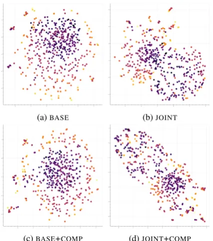
In order to visualize the relation matrices learned by our joint and base models, we use UMAP7 (McInnes and Healy, 2018) to embedMr into a

2D plane8. We use relation matrices trained on

6

Cosine similarity 0.338 is still high for matrices, due to the high dimensionality of their parameter space.

7

https://github.com/lmcinnes/umap

8_{UMAP is a recently proposed manifold learning}

(a)BASE (b)JOINT

(c)BASE+COMP (d)JOINT+COMP

Figure 3: By UMAP, relation matrices are embed-ded into a 2D plane. Colors show frequencies of relations; and lighter color means more frequent.

FB15k-237, and compare models trained by the same number of epochs. The results are shown in Figure3.

We can see that Figure 3a and Figure 3c are mostly similar, with high frequency relations scat-tered randomly around a low frequency cluster, sug-gesting that they come from various directions of a high dimension space, with frequent relations prob-ably being pulled further by the training updates. On the other hand, in Figure3band Figure3dwe found less frequent relations being clustered with frequent ones, and multiple traces of low dimen-sion structures. It suggests that joint training with an autoencoder indeed drives relations toward a low dimension manifold. In addition, Figure 3d

shows different structures against Figure3b, which we conjecture could be related to compositional constraints discovered by compositional training.

Compositional constraints

In order to directly evaluate a model’s ability to find compositional constraints, we extracted from FB15k-237 a list of (r1/r2, r3) pairs such that r1/r2matchesr3. Formally, the list is constructed

as below. For any relationr, we define acontent setC(r)as the set of(h, t)pairs such thathh, r, ti is a fact in the KB. Similarly, we defineC(r1/r2)

t-SNE (van der Maaten and Hinton,2008) but found UMAP more insightful.

Model MR MRR

JOINT+COMP 130±27 .0481±.0090

BASE+COMP 150±3 .0280±.0010

RANDOMM2 181±19 .0356±.0100

Table 3: Performance at discovering compositional constraints extracted from FB15k-237

as the set of(h, t) pairs such thathh, r1/r2, tiis

a path. We regard(r1/r2, r3)as a compositional

constraint if their content sets are similar; that is, if |C(r1/r2)∩C(r3)| ≥ 50 and the Jaccard

similarity betweenC(r1/r2)andC(r3) is≥ 0.4.

Then, after filtering out degenerated cases such as

r1 = r3 orr2 = r₁−1, we obtained a list of 154

compositional constraints, e.g.

(currency of country/country of film,

currency of film budget).

For each compositional constraint(r1/r2, r3)in

the list, we take the matrices M1, M2 and M3

corresponding to r1, r2 and r3 respectively, and

rankM3 according to its cosine similarity with

M1M2, among all relation matrices. Then, we

cal-culate MR and MRR for evaluation. We compare theJOINT+COMPmodel toBASE+COMP, as well as a randomized baseline whereM2is selected

ran-domly from the relation matrices inJOINT+COMP instead (RANDOMM2). The results are shown in Table 3. We have evaluated 5 different random initializations for each model, trained by the same number of epochs, and we report the mean and standard deviation. We verify thatJOINT+COMP performs better thanBASE+COMP, indicating that joint training with an autoencoder indeed helps dis-covering compositional constraints. Furthermore, the random baseline RANDOMM2 tests a hypothe-sis that joint training might be just clusteringM3

andM1here, to the extent thatM3andM1are so

close that even a randomM2 can give the correct

answer; but as it turns out, JOINT+COMP largely outperforms RANDOMM2, excluding this possibil-ity. Thus, joint training performs better not simply because it clusters relation matrices; it learns com-positions indeed.

6.3 Losses and Gains

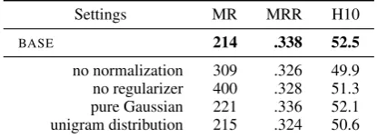
Settings MR MRR H10

BASE 214 .338 52.5

no normalization 309 .326 49.9 no regularizer 400 .328 51.3 pure Gaussian 221 .336 52.1 unigram distribution 215 .324 50.6

Table 4: Ablation of the four settings of the base model as described in Sec.4.1

Crucial settings for the base model

It is noteworthy that our base model already achieves strong results. This is due to several detailed but crucial settings as we discussed in Sec.4.1; Table4shows their gains on the FB15k-237 validation data. The most dramatic improve-ment comes from the regularizer that drives matri-ces to orthogonal.

Gains with compositional training

One can force a model to focus more on (longer) compositions of relations, by sampling longer paths in compositional training. Since joint training with an autoencoder helps discovering compositional constraints, we expect it to be more helpful when the sampled paths are longer. In this work, path lengths are sampled from a Poisson distribution, we thus vary the meanλof the Poisson to control the strength of compositional training. The results on FB15k-237 are shown in Table5.

We can see that, asλgets larger, MR improves much but MRR slightly drops. It suggests that in FB15k-237, composition of relations might mainly help finding more appropriate candidates for a miss-ing entity, rather than pinpointmiss-ing a correct one. Yet, joint training improves base models even more as the paths get longer, especially in MR. It further supports our conjecture that joint training with an autoencoder may strongly interact with composi-tional training.

7 Conclusion

We have investigated a dimension reduction tech-nique which trains a KB embedding model jointly with an autoencoder. We have developed new train-ing techniques and achieved state-of-the-art results on several KBC tasks with strong improvements in Mean Rank. Furthermore, we have shown that the autoencoder learns low dimension sparse cod-ings that can be easily explained; the joint training technique drives high-dimensional data toward low

Model λ Valid Test

MR MRR H10 MR MRR H10

BASE 0 209 .341 52.9 215 .337 52.3

JOINT 0 +1 -.001 -.2 -3 -.001 0

BASE 0.5 204 .337 52.2 211 .332 51.7

JOINT 0.5 -3 +.002 +.1 +1 +.002 +.2

BASE 1.0 191 .334 52.0 203 .328 51.5

JOINT 1.0 -5 +.002 -.1 -6 +.003 +.1

Table 5: Evaluation ofBASEand gains byJOINT, on FB15k-237 with different strengths of composi-tional training. Bold numbers are improvements.

dimension manifolds; and the reduction of dimen-sionality may interact strongly with composition, help discovering compositional constraints and ben-efit from compositional training. We believe these findings provide insightful understandings of KB embedding models and might be applied to other neural networks beyond the KBC task.

Acknowledgments

This work was supported by JST CREST Grant Number JPMJCR1301, Japan. We thank Pontus Stenetorp, Makoto Miwa, and the anonymous re-viewers for many helpful advices and comments.

References

S¨oren Auer, Christian Bizer, Georgi Kobilarov, Jens Lehmann, Richard Cyganiak, and Zachary G. Ives.

2007. Dbpedia: A nucleus for a web of open data.

In The Semantic Web, 6th International Semantic Web Conference, 2nd Asian Semantic Web Confer-ence, ISWC 2007 + ASWC 2007, Busan, Korea, November 11-15, 2007., pages 722–735.

Jonathan Berant, Andrew Chou, Roy Frostig, and Percy

Liang. 2013. Semantic parsing on Freebase from

question-answer pairs. InProceedings of the 2013 Conference on Empirical Methods in Natural Lan-guage Processing, pages 1533–1544, Seattle, Wash-ington, USA. Association for Computational Lin-guistics.

Kurt D. Bollacker, Colin Evans, Praveen Paritosh, Tim Sturge, and Jamie Taylor. 2008. Freebase: a collab-oratively created graph database for structuring hu-man knowledge. InProceedings of the ACM SIG-MOD International Conference on Management of Data, SIGMOD 2008, Vancouver, BC, Canada, June 10-12, 2008, pages 1247–1250.

Antoine Bordes, Nicolas Usunier, Alberto Garc´ıa-Dur´an, Jason Weston, and Oksana Yakhnenko.

2013. Translating embeddings for modeling

Processing Systems 26: 27th Annual Conference on Neural Information Processing Systems 2013. Pro-ceedings of a meeting held December 5-8, 2013, Lake Tahoe, Nevada, United States., pages 2787– 2795.

L´eon Bottou. 2012. Stochastic gradient descent tricks. InNeural Networks: Tricks of the Trade, pages 421– 436. Springer.

Rajarshi Das, Arvind Neelakantan, David Belanger,

and Andrew McCallum. 2017. Chains of

reason-ing over entities, relations, and text usreason-ing recurrent neural networks. InProceedings of the 15th Con-ference of the European Chapter of the Association for Computational Linguistics: Volume 1, Long

Pa-pers, pages 132–141, Valencia, Spain. Association

for Computational Linguistics.

Tim Dettmers, Minervini Pasquale, Stenetorp

Pon-tus, and Sebastian Riedel. 2018. Convolutional 2d

knowledge graph embeddings. In Proceedings of the 32th AAAI Conference on Artificial Intelligence.

John C. Duchi, Elad Hazan, and Yoram Singer. 2011.

Adaptive subgradient methods for online learning and stochastic optimization. Journal of Machine Learning Research, 12:2121–2159.

Dumitru Erhan, Yoshua Bengio, Aaron C. Courville, Pierre-Antoine Manzagol, Pascal Vincent, and Samy

Bengio. 2010. Why does unsupervised pre-training

help deep learning? Journal of Machine Learning Research, 11:625–660.

Michael Gutmann and Aapo Hyv¨arinen. 2012.

Noise-contrastive estimation of unnormalized statistical models, with applications to natural image statistics.

Journal of Machine Learning Research, 13:307– 361.

Kelvin Guu, John Miller, and Percy Liang. 2015.

Traversing knowledge graphs in vector space. In

Proceedings of the 2015 Conference on Empirical Methods in Natural Language Processing, pages 318–327, Lisbon, Portugal. Association for Compu-tational Linguistics.

Katsuhiko Hayashi and Masashi Shimbo. 2017. On

the equivalence of holographic and complex embed-dings for link prediction. In Proceedings of the 55th Annual Meeting of the Association for Compu-tational Linguistics (Volume 2: Short Papers), pages 554–559, Vancouver, Canada. Association for Com-putational Linguistics.

Ben Hixon, Peter Clark, and Hannaneh Hajishirzi.

2015. Learning knowledge graphs for question

an-swering through conversational dialog. In Proceed-ings of the 2015 Conference of the North Ameri-can Chapter of the Association for Computational Linguistics: Human Language Technologies, pages 851–861, Denver, Colorado. Association for Com-putational Linguistics.

Rudolf Kadlec, Ondrej Bajgar, and Jan Kleindienst.

2017.Knowledge base completion: Baselines strike

back. InProceedings of the 2nd Workshop on Rep-resentation Learning for NLP, pages 69–74, Vancou-ver, Canada. Association for Computational Linguis-tics.

Yankai Lin, Zhiyuan Liu, Huanbo Luan, Maosong Sun,

Siwei Rao, and Song Liu. 2015a. Modeling relation

paths for representation learning of knowledge bases. In Proceedings of the 2015 Conference on Empiri-cal Methods in Natural Language Processing, pages 705–714, Lisbon, Portugal. Association for Compu-tational Linguistics.

Yankai Lin, Zhiyuan Liu, Maosong Sun, Yang Liu, and

Xuan Zhu. 2015b. Learning entity and relation

em-beddings for knowledge graph completion. In Pro-ceedings of the Twenty-Ninth AAAI Conference on Artificial Intelligence, January 25-30, 2015, Austin, Texas, USA., pages 2181–2187.

Laurens van der Maaten and Geoffrey Hinton. 2008.

Visualizing data using t-SNE. Journal of Machine Learning Research, 9:2579–2605.

L. McInnes and J. Healy. 2018. UMAP: Uniform

Man-ifold Approximation and Projection for Dimension Reduction.ArXiv e-prints.

Tomas Mikolov, Wen-tau Yih, and Geoffrey Zweig.

2013. Linguistic regularities in continuous space

word representations. In Proceedings of the 2013 Conference of the North American Chapter of the Association for Computational Linguistics: Human Language Technologies, pages 746–751, Atlanta, Georgia. Association for Computational Linguistics.

George A. Miller. 1995. Wordnet: A lexical database

for english.Commun. ACM, 38(11):39–41.

Vinod Nair and Geoffrey E. Hinton. 2010. Rectified

linear units improve restricted boltzmann machines. InProceedings of the 27th International Conference on Machine Learning (ICML-10), June 21-24, 2010, Haifa, Israel, pages 807–814.

Arvind Neelakantan, Benjamin Roth, and Andrew

Mc-Callum. 2015. Compositional vector space

mod-els for knowledge base completion. InProceedings of the 53rd Annual Meeting of the Association for Computational Linguistics and the 7th International Joint Conference on Natural Language Processing (Volume 1: Long Papers), pages 156–166, Beijing, China. Association for Computational Linguistics.

Dat Quoc Nguyen, Kairit Sirts, Lizhen Qu, and Mark

Johnson. 2016. Stranse: a novel embedding model

of entities and relationships in knowledge bases. In

Maximilian Nickel, Kevin Murphy, Volker Tresp, and

Evgeniy Gabrilovich. 2016a. A review of relational

machine learning for knowledge graphs. Proceed-ings of the IEEE, 104(1):11–33.

Maximilian Nickel, Lorenzo Rosasco, and Tomaso A.

Poggio. 2016b. Holographic embeddings of

knowl-edge graphs. InProceedings of the Thirtieth AAAI Conference on Artificial Intelligence, February 12-17, 2016, Phoenix, Arizona, USA., pages 1955– 1961.

Maximilian Nickel, Volker Tresp, and Hans-Peter

Kriegel. 2011. A three-way model for collective

learning on multi-relational data. InProceedings of the 28th International Conference on International Conference on Machine Learning, ICML’11, pages 809–816, USA. Omnipress.

Sebastian Riedel, Limin Yao, Andrew McCallum, and

Benjamin M. Marlin. 2013.Relation extraction with

matrix factorization and universal schemas. In Pro-ceedings of the 2013 Conference of the North Amer-ican Chapter of the Association for Computational Linguistics: Human Language Technologies, pages 74–84, Atlanta, Georgia. Association for Computa-tional Linguistics.

R. Rubinstein, A. M. Bruckstein, and M. Elad. 2010.

Dictionaries for sparse representation modeling.

Proceedings of the IEEE, 98(6):1045–1057.

Michael Sejr Schlichtkrull, Thomas N. Kipf, Peter Bloem, Rianne van den Berg, Ivan Titov, and Max

Welling. 2017. Modeling relational data with graph

convolutional networks.CoRR, abs/1703.06103.

Yelong Shen, Po-Sen Huang, Ming-Wei Chang, and

Jianfeng Gao. 2017. Modeling large-scale

struc-tured relationships with shared memory for knowl-edge base completion. In Proceedings of the 2nd Workshop on Representation Learning for NLP, pages 57–68, Vancouver, Canada. Association for Computational Linguistics.

Baoxu Shi and Tim Weninger. 2017. Proje:

Embed-ding projection for knowledge graph completion. In

Proceedings of the Thirty-First AAAI Conference on Artificial Intelligence, February 4-9, 2017, San Fran-cisco, California, USA., pages 1236–1242.

Carina Silberer and Mirella Lapata. 2014.

Learn-ing grounded meanLearn-ing representations with autoen-coders. In Proceedings of the 52nd Annual Meet-ing of the Association for Computational LMeet-inguis- Linguis-tics (Volume 1: Long Papers), pages 721–732, Balti-more, Maryland. Association for Computational Lin-guistics.

Richard Socher, Danqi Chen, Christopher D. Manning,

and Andrew Y. Ng. 2013. Reasoning with neural

tensor networks for knowledge base completion. In

Advances in Neural Information Processing Systems 26: 27th Annual Conference on Neural Information

Processing Systems 2013. Proceedings of a meet-ing held December 5-8, 2013, Lake Tahoe, Nevada, United States., pages 926–934.

Richard Socher, Jeffrey Pennington, Eric H. Huang, Andrew Y. Ng, and Christopher D. Manning. 2011.

Semi-supervised recursive autoencoders for predict-ing sentiment distributions. InProceedings of the 2011 Conference on Empirical Methods in Natural Language Processing, pages 151–161, Edinburgh, Scotland, UK. Association for Computational Lin-guistics.

Ran Tian, Naoaki Okazaki, and Kentaro Inui. 2016.

Learning semantically and additively compositional distributional representations. InProceedings of the 54th Annual Meeting of the Association for Compu-tational Linguistics (Volume 1: Long Papers), pages 1277–1287, Berlin, Germany. Association for Com-putational Linguistics.

Ivan Titov and Ehsan Khoddam. 2015. Unsupervised

induction of semantic roles within a reconstruction-error minimization framework. In Proceedings of the 2015 Conference of the North American Chap-ter of the Association for Computational Linguistics: Human Language Technologies, pages 1–10, Den-ver, Colorado. Association for Computational Lin-guistics.

Kristina Toutanova and Danqi Chen. 2015. Observed

versus latent features for knowledge base and text inference. InProceedings of the 3rd Workshop on Continuous Vector Space Models and their Composi-tionality, pages 57–66, Beijing, China. Association for Computational Linguistics.

Kristina Toutanova, Victoria Lin, Wen-tau Yih,

Hoi-fung Poon, and Chris Quirk. 2016. Compositional

learning of embeddings for relation paths in knowl-edge base and text. InProceedings of the 54th An-nual Meeting of the Association for Computational Linguistics (Volume 1: Long Papers), pages 1434– 1444, Berlin, Germany. Association for Computa-tional Linguistics.

Th´eo Trouillon, Johannes Welbl, Sebastian Riedel, ´Eric

Gaussier, and Guillaume Bouchard. 2016. Complex

embeddings for simple link prediction. In Proceed-ings of the 33nd International Conference on Ma-chine Learning, ICML 2016, New York City, NY, USA, June 19-24, 2016, pages 2071–2080.

Quan Wang, Zhendong Mao, Bin Wang, and Li Guo.

2017. Knowledge graph embedding: A survey of

approaches and applications. IEEE Trans. Knowl. Data Eng., 29(12):2724–2743.

Zhen Wang, Jianwen Zhang, Jianlin Feng, and Zheng

Chen. 2014a. Knowledge graph and text jointly

Zhen Wang, Jianwen Zhang, Jianlin Feng, and Zheng

Chen. 2014b. Knowledge graph embedding by

translating on hyperplanes. In Proceedings of the Twenty-Eighth AAAI Conference on Artificial Intel-ligence, July 27 -31, 2014, Qu´ebec City, Qu´ebec, Canada., pages 1112–1119.

Han Xiao, Minlie Huang, and Xiaoyan Zhu. 2016.

From one point to a manifold: Knowledge graph em-bedding for precise link prediction. InProceedings of the Twenty-Fifth International Joint Conference on Artificial Intelligence, IJCAI 2016, New York, NY, USA, 9-15 July 2016, pages 1315–1321.

Qizhe Xie, Xuezhe Ma, Zihang Dai, and Eduard Hovy.

2017. An interpretable knowledge transfer model

for knowledge base completion. In Proceedings of the 55th Annual Meeting of the Association for Computational Linguistics (Volume 1: Long Papers), pages 950–962, Vancouver, Canada. Association for Computational Linguistics.

Bishan Yang, Wen-tau Yih, Xiaodong He, Jianfeng

Gao, and Li Deng. 2015. Embedding Entities and

Relations for Learning and Inference in Knowledge Bases. InProceedings of the 3rd International Con-ference on Learning Representations, pages 1–12.

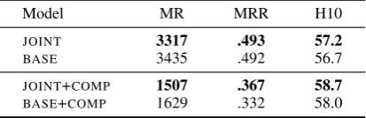
A Out-of-vocabulary Entities in KBC

Occasionally, a KBC test set may contain entities that never appear in the training data. Such out-of-vocabulary (OOV) entities pose a challenge to KBC systems; while some systems address this issue by explicitly learn an OOV entity vector (Dettmers et al.,2018), our approach is described below. For an incomplete triplehh, r,?iin the test, ifhis OOV, we replace it with the most frequent entity that has ever appeared as a head of relationrin the training data. If the gold tail entity is OOV, we use the zero vector for computing the score and the rank of the gold entity.

Usually, OOV entities are rare and negligible in evaluation; except for the WN18RR test data which contains about 6.7% triples with OOV en-tities. Here, we also report adjusted scores on WN18RR in the setting that all triples with OOV entities are removed from the test. The results are shown in Table6.

Model MR MRR H10

JOINT 3317 .493 57.2

BASE 3435 .492 56.7

JOINT+COMP 1507 .367 58.7

BASE+COMP 1629 .332 58.0