http://dx.doi.org/10.4236/msa.2013.41010 Published Online January 2013 (http://www.scirp.org/journal/msa)
FE Modeling and Analysis of Isotropic and Orthotropic
Beams Using First Order Shear Deformation Theory
M. Adnan Elshafei*
Aeronautical Department, Military Technical Collage, Cairo, Egypt. Email: *[email protected]
Received October 26th, 2012; revised November 12th, 2012; accepted December 11th, 2012
ABSTRACT
In the present work, a finite element model is developed to analyze the response of isotropic and orthotropic beams, a common structural element for aeronautics and astronautic applications. The assumed field displacements equations of the beams are represented by a first order shear deformation theory, the Timoshenko beam theory. The equations of motion of the beams are derived using Hamilton’s principle. The shear correction factor is used to improve the obtained results. A MATLAB code is constructed to compute the natural frequencies and the static deformations for both types of beams with different boundary conditions. Numerical calculations are carried out to clarify the effects of the thick- ness-to-length ratio on both the Eigen values and the deflections of the beams due to the applied mechanical load. The obtained results of the proposed model are compared to the available results of other investigators, good agreement is generally obtained.
Keywords: Finite Element Method; Timoshenko Beam Theory; Composite Materials Mechanics; Static and Dynamic Analysis of Beams
1. Introduction
The current trend of aeronautics and astronautic design is to use large, complex, and light-weight structures ele- ments. These structures are commonly having low-fre- quency fundamental vibration modes in addition to fab- ricate by graphite-epoxy to satisfy the requirements of minimum weight and low thermal distortion. Because of that several researchers are interested to solve the beam structures by different theories.
Yuan and Miller [1], proposed finite element model for laminated composite beams with separate rotational degrees of freedom for each lamina. The shear deforma- tion is included in the model but the interfacial slip or de- lamination is not included. Their element can be used even for short beams with many laminas. The model re- sults was compared with those of other theoretical and experimental investigations and found reasonable.
Chandrashekhara and Bangera [2], developed finite element model based on a higher-order deformation the- ory with Poisson’s effect is incorporated. They conclud- ed the following: 1) The shear deformations decrease the natural frequencies of the beam; 2) The natural frequen- cies increase with the increase of the number of beam layers; 3) The clamped-free boundary condition exhibits
the lowest frequencies; 4) The increase of fiber orienta- tion angle decreases the natural frequency; and 5) the natural frequency decreases by increasing the material anisotropy.
Friedman and Kosmatka [3], developed two-node Ti- moshenko beam element using Hamilton’s principal. The resulting stiffness matrix of their model was exactly in- tegrated and it was free of “shear-locking”, and it was in agreement with the exact Timoshenko beam stiffness matrix. Their element was exactly predicting the dis- placement of short beam subjected to distributed loads and also predicted the natural frequencies.
Lidstrom [4], derived an equilibrium formulation of 3D beam element using the energy derivatives. His for- mulation contains the coupling terms between translation and twist, also between translational bending and elonga- tion. A three node element was introduced in such model. Also condensed two node version of the element has been analyzed. He found that two-node system was less numerically stable than the proposed three-node system.
Bhate et al. [5], proposed a refined flexural theory for composite beam based on the potential energy concept. The warping effect is included in their formulation; however the shear correction coefficient was eliminated. They found that their theory is established for short composite beams where cross-sectional warping is pre- dominant.
Nabi and Ganesan [6], studied the free vibration char- acteristics of composite beams using finite element mo- del based on a first-order deformation theory including bi-axial bending as well as torsion. They studied the ef- fect of shear-deformation, beam geometry, and bound- ary conditions on the natural frequencies. They con- cluded that the natural frequencies are 1) Decrease with the increase of fiber orientation angle; 2) Increase with the increase of the beam length to height ratio for all fi- ber orientation angles; 3) Also have the lowest value in case of clamped-free boundary conditions
Armanios and Badir [7], evaluated analytically the ef- fect of elastic coupling mechanisms on vibration behave- ior of thin-walled composite beams. Good agreement was found between their results and those developed by Giavotto et al. (1983) [8], and Hagodes et al. (1991) [9], based on finite element technique, and the experimental measurements obtained by Chandra and Chopra [10].
Rao and Ganesan [11], investigated a Harmonic re- sponse of tapered composite beams using finite element model based on a higher order shear deformation theory. The uniaxial bending and the Poisson ratio effect were considered and the interlaminar shear stresses were ne-glected. The effect of in-plane inertia and rotary inertia were also considered in their formulation of the mass matrix. A parametric study is done of the influence of anisotropy, taper profile and taper parameter. They found that the transversal displacement is higher than that of a uniform beam. For the taper parameter effect, they de-duced that the frequency decreases with increase thick-ness variations and vise-verse.
Khdeir and Reddy [12], presented an exact solution of the governing equations for the bending of laminated beams. They used the classical, the first-order, the sec- ond-order, and the third-order beam theories in their analysis. They studied the effect of shear deformation, number of layers, and the orthotropic ratio on the static response of composite beams. They found large differ- ences between the predicted deflections by the classical beam theory and the higher order beam theories, espe- cially when the ratio of beam length to its height was low due to the shear deformation effects.
Yildirim et al. [13], studied the in-plane free vibration of laminated beams based on the transfer matrix method. They considered rotary inertia, shear, and extensional deformation effects on the Timoshenko’s beam analysis. Good predictions are obtained and compared to other reporters for different modes of the natural frequencies.
Chakraborty et al. [14], proposed a refined looking free first order shear deformable finite element model to solve free vibration and wave propagation problems in laminated composite beam. They developed element, that its shape functions is dependent not only on the length of
the element, but also on its material and cross-sectional properties. The developed stiffness matrix is exact while the mass distribution is approximate. Rotary inertia and effect of geometric and material asymmetry is taken into account. They named the model as refined first order deformable element (RFSDE).
Eisenberger [15], proposed exact stiffness coefficients for isotropic beam using a simple higher order theory, which include cubic variation of the axial displacements over the cross-section of the beam. Their model had three degrees of freedom at each node, one transverse displace- ment and two rotations. They compared their model re- sults with Bernoulli-Euler and Timoshenko beam models and found acceptable.
Lee and Schultz [16], studied the free vibration of Ti- moshenko beams and axi-symmetric Mindlin plates. The analysis was based on the Chebyshev pseudospectral me- thod, which has been widely used in the solution of fluid mechanics problems. Different boundary conditions of Ti- moshenko beams were treated, and numerical results were presented for different thickness-to-length ratios.
Subramanian [17], proposed free vibration analysis of composite beams using Finite elements based on two higher order shear deformation theories. The difference between the two theories is that the first theory assumed a non-parabolic variation of transverse shear stress across the thickness of the beams whereas the second theory assumed parabolic variation. The comparison study showed that natural frequencies predict by his model were better than those obtained by other theories and the considered finite elements.
Simsek and Kocaturk [18], studied the free vibration of isotropic beams based on the third-order shear defor- mation theory. The boundary conditions are satisfied using Lagrange multipliers which reduced the solution of a system of algebraic equations. A trial functions for the deflections and rotations of the cross-section of the beam are expressed in polynomial form. Their results are compared with the previous results based on CBT and FSDT.
Jun et al. [19], proposed dynamic finite element model for beams based of first-order shear deformation theory. They introduced the influences of Poisson effect, cou- plings among extensional, bending and torsion deforma- tions, shear deformation and rotary inertia in their for- mulation. Their obtained results are compared to those previously published and founded in good accuracy.
solutions, while reducing the total number of degrees- of-freedom to resolve the computational and cost prob- lems.
Nguyen et al. [21], presented full closed-form solution of the governing equations of two-layer composite beam. Timoshenko’s kinematics assumptions are considered for both layers and the shear connection is modeled through a continuous relationship between the interface shear flow and the corresponding slip. They derived the “ex- act” stiffness matrix using the direct stiffness method. They found that the effect of shear flexibility on the de- flection is generally more important for composite beams characterized by substantial shear interaction.
Lina and Zhang [22], proposed a two-node element with only two degrees of freedom per node for finite element analyses of isotropic and composite beams. Their model was based on Timoshenko theory. They concluded that their proposed model is accurate and computationally efficient for analysis of isotropic and composite beams.
Kennedya et al. [23], presented Timoshenko beam theory for layered orthotropic beams. The proposed the- ory yields Cowper’s shear correction for single isotropic layer, while for multiple layers new expressions for the shear correction factor are obtained. The body-force cor- rection was shown to account for the difference between Cowper’s shear correction and the factor originally pro- posed by Timoshenko. Numerical comparisons between the theory and finite-elements results showed good agree- ment.
In the present work, a finite element model is proposed, based on first order shear deformation theory, Timo- shenko beam theory, with a shear correction factor, to predict the static responses and dynamic characteristics of advanced isotropic and orthotropic beams for different boundary conditions and different length to thickness ratio due to different applied loads. The structure outline of the present work can be drawn for both isotropic and orthotropic beams as follows:
1) Theoretical formulation using the Timoshenko the- ory.
2) Finite element formulation to obtain the structure equation of motion.
3) The model validation and parametric studies which contain the items:
a) Model convergence for both deflection and eigen- values.
b) Static deformation of the beam. c) Dynamic characteristics of the beam. d) Model predictions analysis and conclusions.
2. Theoretical Formulation
The displacements field equations of the beam are as- sumed as follows [12]:
1
3 2
2 3
d ,
d
d d
o o
w
u x z u x z c c x
x
z w
c z x c x
h x
(1a)
,v x z 0 (1b)
, o
w x z w x
(1c) where , and are the displacements field equa- tions along the coordinatesu v w
,
x yand , respectively, and 0 denote the displacements of a point
z u0
w
x y, , 0
at the mid plane,
x
x and
x are the rota- tion angles of the cross-section as shown in Figure 1.By selecting the constant values of Equation (1) a as:
0 0,
c c11, c20, 3 , the displacements field equations for first-order theory (FOBT) at any point through the thickness can be expressed as [24]:
0
c
,
, 0
,
o o u x z u x z x
v x z w x z w x
(2)
The strain-displacement relationships are obtained by differentiating the assumed displacement field equations, Equation (2), as follows:
, , , ,
, ,
xx
o o
xx x u x y z
x y z
x
u x z x z
z z
x x
x
(3a)
, ,
, ,
, ,
d d xz
o
x xz
u x y z w x y z x y z
x x
w x
(3b)
The strains at any point through the thickness of the beam can be written in matrix form as:
xx xx xz
xx xz x
z
z
(4)
The components xx xz and xxare the reference
surface extensional strain in the x-direction, in-plane shear strain, and curvature in the x-direction, respec- tively.
The generalize stress strain relationship is given by [25]:
ij cijkl kl
(5)
where, i j, 1,,6; and k1,, 3.
k 11 12 11 11 12 22 22 22 44 23 23 55 13 13 66 12 12
0 0 0
0 0 0
0 0 0 0
0 0 0 0
0 0 0 0
k k Q Q Q Q Q Q Q
related to the engineering constants for two material cases such as:
(6) Case I: Isotropic Beam
11 22 2
1
k k E
Q Q
12 2
1
k E
Q
44 55 66
k k k
Q Q Q G (7a) where; E , G, and are the material properties. where, Qijare the reduced stiffness components which Case II: Orthotropic Beam
1 12 2 2
11 12 22 44 23 55 13 66 12
12 21 12 21 12 21
1 1 1
k k k k
k k k k k k k
k k k k k k
E E E
Q Q Q Q G Q G Q
k
G
(7b)
3. Energy Formulation
where; Ei is the modules in xi direction, G iij
j
are the shear modules in the xixj plane, and ij are
the associated Poisson’s ratios. The kinetic energy of the beam structure is given by [6]: Thus the transformed stress-strain relationship can be
written as:
11 12 16
21 22 26
44 45 45 55
16 26 66
0 0
0 0
0 0 0
0 0 0
0 0
xx xx
yy yy
yz yz
xz xz
xy k xy
Q Q Q
Q Q Q
Q Q
Q Q
Q Q Q
k k
(8)
2 2
1
d 2v
T
u w v (10) where, ρ is the mass density of the material of the beam.The internal strain energy for the beam structure is represented by [12]:
U
1
d 2v xx xx xz xz U
viw
(11)
And the work done due to external loads is represented by [24]:
where, Qij, are the transformed reduced stiffness com-
ponents [25].
0 0
d d
L L
a t
W
f u x
f w x P i (12) In the present model the width in y direction is stressfree and a plane stress assumptions are used. Therefore, it is possible to setyy yz xy yz xy0, and
0
yy
in Equation (8). Therefore, the stress-strain rela- tionship can be reduced to:
where; fa, and ft are the transversal and axial forces
along a surface with length , respectively. i, is the
concentrated force at point and is the corre- sponding generalized displacement.
L i P i w 11 55 0 0 xx xx
xz s x
Q
k Q z
(9a) Case I: Isotropic beam
By substituting Equations (9a), and (9b) into Equa- tion (11), the internal strain energy is represented by: where; ks is the shear correction factor and the coeffi-
cients in Equation (9a) are given by:
2 21
d
2v xx s xz
U
E k G
v (13) Case I: Isotropic beam11 55 , and ij ij
Q E Q G Q Q (9b)
By inserting Equations (3a), and (3b) into Equation (13), one can obtain:
Case II: Orthotropic Beam
2 d 21
d
2 d
o
xx xx s x
v
w
U E z k G
x
12 1211 11 55 55
22 Q Q
Q Q Q Q
Q
(9c) v (14a)
22 2
2 d d
1
2 2
2 d
o o xx xx xx xx s x x
v
w w
U E z z k G
x x
dd v (14b) Thus;
2 2
2 2
d d d d d d
1
2 2
2 d d d d x d d
o o x x o o
s x
v
u u w w
U E zE z E k G
x x x x x x
2 dv (15)
Case II: Orthotropic Beam
2 211 55
1
d
2v xx s xz
U
Q k Q
v (16)By inserting Equations (3a), and (3b) into Equation (16),
one can obtain:
2 2 11 55 d 1 d 2 d oxx xx s x
v
w
U Q z k Q
x
v
(17a)
22 2 2
11 55 d d 1 2 2 2 d o o xx xx xx xx s x x
v
w w
U Q z z k Q
x x
dd v (17b) And performing the integration through the thickness, the internal strain energy for anisotropic beam is represented by:
2 2
2
2
11 11 11 55
2 0
d d d d d d
1
2 2
2 d d d d d d
b L
o o x x o o
s x x
b
u u w w
U A B D k A
x x x x x x
2d dx y (18)
where, A Bij, ij,and are the laminate extensional, coupling, and bending stiffness coefficients and they are given by [25]: ij D
2 211 11 11 1 55 55 55 1
1 1
2 2
2 2
2 2 2 3 3
11 11 11 1 11 11 11 1
1 1 2 2 d d 1 1 d d 2 3
h N h N
k k k k
k k k k
k k
h h
h N h N
k k k k
k k k k k k
h h
A Q z Q z z A Q z Q z z
B Q z z Q z z D Q z z Q z z
(19)4. Finite Element Formulation
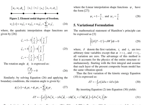
In the present model the proposed element has five nodes with nine degrees of freedom representing the deforma- tions u w, , and x as shown in the Figure 2.
A cubic shape functions are used to represent the axial displacementu, quadratic shape functions for the trans- verse displacement
w
, where the rotation x is repre-sented by a linear shape functions, this will result a nine by nine stiffness matrix with different degrees of freedom at different nodes [24]. From these selections we have:
d
Linear Linear d o x w x
, and
2
d d quadratic quadratic d d o o u w x x
Which satisfied the constrains, shear strain
0
constant xz
, and membrane strain , to avoid
the error in the finite element analysis which is known as shear Locking due to un-accurately models the curvature present in the actual material under bending, and a shear stress is introduced. The additional shear stress in the element causes the element to reach equilibrium with smaller displacement, i.e., it makes the element appear to be stiffer than it actually is and gives bending displace- ments smaller than they should be. The axial displace- ment at the mid-plane is expressed as the following:
0 xx 0 u 4 4 0 o u x
(20) By solving the previous equation and imposing the boundary conditions, the axial displacement can be rep- resented as:
41 1 2 2 3 3 4 4 1
o j
j u x u u u u u j
(21)where the cubic shape functions j are found to be [26]:
3 2 1 3 2 2 3 2 3 3 2 4 9 11 9 1 2 2 27 45 9 2 2 27 9 18 2 2 9 9 2 2
x x x
L L L
x x x
L L L
x x x
L L L
x x x
L L L
(22)
The transversal displacement wis represented as:
3 3 0 o w x
(23) By solving the above equation and applying the boundary conditions to determine the unknown constants, the transversal displacement can be expressed in terms of the nodal displacement as:
[image:5.595.331.513.614.710.2]w
z x o w o u xz x o dw dx o dw dx
u w1, 1,x1
u2 2w
3
[image:6.595.54.544.67.430.2]u
u w4, 3,x2
Figure 2. Element nodal degrees of freedom.
31 1 2 2 3 3 1
o
j w x w w w wjj
(24)where, the quadratic interpolation shape functions are given by [26]:
2
1
2
2
2
3
1 3 2
4 4
2
x x
L L
x x
L L
x x
L L
(25)
The rotation angle x is expressed as: 2
2 0
x
x
(26) Similarly; by solving Equation (26) and applying the boundary conditions, the rotation angle is given by:
21 1 2 2 1
x x x xj
j
x
where the Linear interpolation shape functions j have
the form [27]:
1 1
x L
, and 2
x L
(28)
5. Variational Formulation
The mathematical statement of Hamilton’s principle can be expressed as [3]:
2
1
d 0
t t
T U W t
(29)where, denote the first variation, and t2 are two arbitrary time variables except that at 1, and 2
1
t
t t t t , all variation are zero. The advantage of this method is that it accounts for the physics of the entire structure si- multaneously. Starting with the first integral and assume that each layer of the present composite beam model has the same vibration speed.
Thus the first variation of the kinetic energy Equation (10) is expressed as:
dv
T u u w w
v
(30)
j
(27)By inserting Equation (2) into Equation (30) yields:
2
d
T T T T T
o o o x x o x x o o v
T u u z u z u z w w
v(31)
By substituting the shape functions Equations. (21), (24), and (27) in Equation (31) the components of the element mass matrix can be expressed by:
11 0 12 13 1
0 0
21 22 0 23 31 1
0 0
2
32 33 2 0 1 2
0
d 1, , 4 0 d 1, , 4 and 1, 2
0 d 1, , 3 0 d 1, 2 and 1, , 4
0 d 1, 2 and , , 1, , d
L L
T T
i i i j
L L
T T
i i i j
L T i i
A
M I x i M M I x i j
M M I x i M M I x i j
M M I x i I I I z z A
(32)
where, Iiis the mass moment of inertia.
By inserting Equations (22), (25), and (28) into Equa- tion (32) and perform the integrating, the element mass matrix is obtained, and given in Appendix A.
The first variation of the external work Equation (12) takes the form:
0 0
d d
i
L L
a o x t o i o
W f u z x f w x P w
By inserting the shape functions Equations. (21), (24), and (27) into Equation (33), one can obtain:
x
d
(33)
0 0
0
d d
d
L L
a i oi a i xi L
t i oi i
W f u x f z
f w x P
(34)
Thus, the elements of the load vector are as follows:
11 1 12 2 13 3 14 4 21 1 1
0 0 0 0 0
22 2 2 23 3 3 31 1 32 2
0 0 0 0
d d d d
d d d d
L L L L L
a a a a t
L L L L
t t a a
F f x F f x F f x F f x F P f x
F P f x F P f x F f z x F f z x
By substituting Equations (22), (25), and (28) in Equa- tion (35) and perform the integrating, the element load vector can be obtained and given in Appendix A.
Case I: Isotropic beam:
By taking the variation of Equation (15), one can ob-tain:
4 4 2 4 4 2
1 1 1 1 1 1
2 2
2
1 1
d d d d d
1
2 2
2 d d d d d d
d d
2
d d
o j oi xj oi o j xi
j i j i j i
v
xj xi
j i
u u u u
U E Ez
x x x x x x
Ez x x
d
2 2 2 3
1 1 1 1
3 2 3 3
1 1 1 1
d 2
d
d d d
d
d d d
oi
s xj xi xj
j i j i
o j o j oi
xi
j i j i
w k G
x
w w w
v
x x x
(36)By substituting Equations (21), (24) and (27) in Equation (36) yields:
4 4 2 4 4 2
1 1 1 1 1 1
2 2
2
1 1
d d d d d
1
2 2
2 d d d d d d
d d
2 2
d d
j i j i j
j i j i j i
v
j i
s
j i
U E Ez
x x x x x x
Ez k G
x x
d i
2 2 2 3
1 1 1 1
3 2 3 3
1 1 1 1
d d
d d d
d
d d d
i
j i j
j i j i
j j i
i
j i j i
x v
x x x
(37)
Equation (37) defines the elements of the stiffness matrix as follows:
4 4 4 2 3 3
11 12 21 13 22
1 1 1 1 1 1
3 2 23 1 1 d d d d d d
d d d d d d
d d d j j i i s
i j i j i j
v v v
i
s j
i j
v
k E v k k k Ez v k k G
x x x x x x
k k G v k
x
d d d ji v
2 4 2 3
31 32
1 1 1 1
4 4 4 2
11 12 21 13
1 1 1 1
d d
d
d d
d d d
d d
d d
d d
d d d d
j j
i
s i
i j i j
v v
j j
i i
i j i j
v v
Ez v k k G v
x x x
k E v k k k Ez v
x x x x
3 3 22 1 13 2 2 4 2 3
23 31 32
1 1 1 1 1 1
d d d d d d d d d d d
d d d d
j i s i j v j j i i
s j s i
i j i j i j
v v v
k k G
x x
k k G v k Ez v k k G v
x x x
dv
x
(38)
By inserting Equation (22), (25) and (28) into Equa- tion (38), and perform the integration, the element stiff- ness matrix for isotropic Timoshenko Beam is obtained
and given in Appendix A. Case II: Orthotropic Beam:
By taking the variation of Equation (18), one can obtain:
2 4 4 2 4 4 2
11 11
1 1 1 1 1 1
2 0
2 2
11
1 1
d d d d d
1
2 2
2 d d d d d
d d
2
d d
b L
j i j i j
j i j i j i
b
j i
j i
U A B
x x x x x x
D x x
d d i
2 2 2 3
55
1 1 1 1
3 2 3 3
1 1 1 1
d 2
d
d d d
d d
d d d
i
s j i j
j i j i
j j i
i
j i j i
k A
x x y
x x x
(39)By inserting Equations (21), (24) and (27) into Equa-tion (39) yields the form given in EquaEqua-tion (40):
By substituting Equation (22), (25) and (28) in Equa- tion (41) and perform the integration, the element stiff- ness matrix of anisotropic Timoshenko beam is obtained and given in Appendix A.
6. Equation of Motion
The system equation of motion is given in matrix form as [11]:
M q
K q
F (42) where
M is the global mass matrix, is the sec- ond derivative of the nodal displacements with respect to time,
q
K is the global stiffness matrix,
q is the nodal displacements vector and
F is the global nodal forces vector.7. Numerical Example and Discussion
A MATLAB code is constructed to perform the analysis of isotropic and orthotropic beams using the present fi- nite element model. The model is capable of predicting the nodal (axial and transversal) deflections and the fun- damental natural frequency of the beam. The model in- puts are the materials and geometric properties of the beams. The shear correction factor is taken as k = 5/6, and the following boundary conditions of the beams are considered as follows:
Simply-supported edge: u0, andw0. Clamped edge: u0, w0, and x0.
The model validation is performed by checking the convergences for deflection and eigen-values, static de-
flections and dynamic characteristics for both isotropic and orthotropic beams.
Case I: Isotropic beam results 1) Model Convergences
The convergence of the present model is checked for the aluminum beam with the material and geometric properties given in Table 1. The beam is subjected to uniform distributed load of intensity 1 N/m. The obtained results are shown in Figure 3, which presents the effect of number of element on the normalized transversal tip deflection of a cantilever beam, with length to height ratio (L/h) of 10, The normalized deflection is given as;
2
10 yy
w w EI L4
. It can be seen from the figure that the model predictions are start to converge at reasonable number of elements.
The convergence of the Eigen values is checked for two cases of the beam boundary conditions clamped-free and clamped-clamped where the dimensionless frequency
is defined as: 2 2
i i m L
EI
, and is the mass
per unit length of the beam.
m
a) Clamped-free aluminum beam with the properties given in Table 1. The obtained dimensionless first natu- ral frequency is conversing by increasing the number of elements as shown in Figure 4.
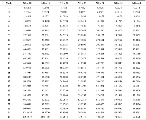
b) Clamped-Clamped aluminum beam with the prop- erties: Poisson’s ratio 0.3 thickness to length ratio is h/L=0.01, and the number of elements are chosen from 10 to 40. The obtained normalized natural frequencies are presented in Table 2 for different number of ele-
2 4 4 2 4 4 2
11 11
1 1 1 1 1 1
2 0
2 2
11
1 1
d d d d d
1
2 2
2 d d d d d
d d
2
d d
b L
j i j i j
j i j i j i
b
j i
j i
U A B
x x x x x x
D x x
d d i
2 2 2 3
55
1 1 1 1
3 2 3 3
1 1 1 1
d 2
d
d d d
d d
d d d
i
s j i j
j i j i
j j i
i
j i j i
k A
x x y
x x x
(40)2 4 4 2 4 2
11 11 12 21 13 11
1 1 1 1
2 0 2 0
2 3 3
22 55 23 55
1 1
2 0
d d
d d
d d d d
d d d d
d d
d d
d d
b L b L
j j
i i
i j i j
b b b L j i s s i j b
k A x y k k k B x
x x x x
k k A x y k k A
x x
y
2 3 2
1 1
2 0
2 2 4 2 2 3
31 11 32 55
1 1 1 1
2 0 2 0
2
33 11 55
1 d d d d d d d
d d d d
d d d
d d d d b L i j i j b
b L b L
j j
i
s i
i j i j
b b
j i
s i j
j
x y x
k B x y k k A x y
x x x
k D k A
x x
2 2 2 2
1` 1 1
2 0
d d
b L
i j i
0 10 20 30 40 50 60 70 80 90 100 0
0.5 1 1.5 2 2.5 3 3.5 4 4.5
5x 10
-5
Number of Elements
N
or
m
al
iz
ed
T
ip D
ef
lec
ti
on
Tip deflection of Cantilever Aluminum beam
Figure 3. Normalized transversal tip displacements vs. number of elements of cantilever aluminum beam.
Table 1. Material and geometric properties for aluminum beam.
Property Aluminum Unit
E 68.9 GPa
V 0.25 -
G 27.6 GPa
2769 (kg/m3)
Length, L 0.1524 (m)
Width, b 0.0254 (m)
Height, h 0.01524 (m)
ments “NE”. The obtained results are found reasonable and compared with the predictions given by [16], which used different numbers of collocation points to determine the size of the problem in their studies It is clear from Figure 4 and Table 2 that as the number of elements increase the natural frequency decreases for the first and other modes.
2) Static Validation Example (1):
A cantilever isotropic beam with cross-section dimen- sionsh b 1,E1, and 1 are used in the valida- tion in order to compared with other references. The beam is subjected to transverse uniform distributed loads with intensity up to 10 N/m, and with different values of length to thickness ratio L/h = 4, 10, 20, 50, and 100. In the present example, the shear correction factor is taken as
1
t
f
5 6
s
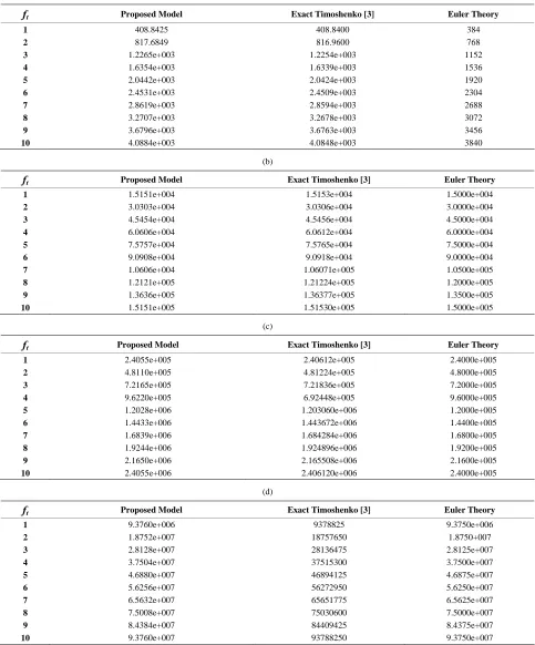
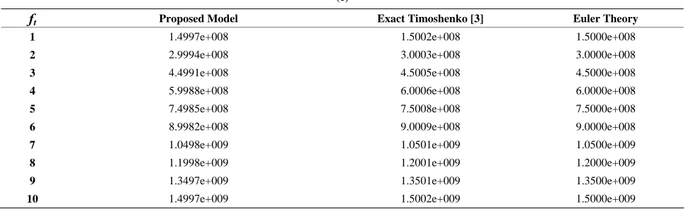
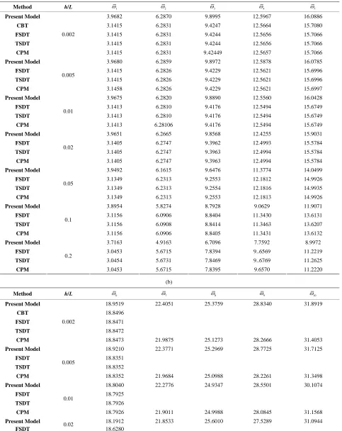
k and number of elements, NE = 33, are taken in the proposed model in order to com- pare the results to other references. The obtained results are presented and in Table 3(a)-(e) and compared to [3], where the Timoshenko–based tip deflection
is given as:
4
1 8
t t
yy
f L W
EI
,
2 1
12 11 5
h
and its shear correction factor is 10 1
12 11 s
k
. Also
compared with the known Euler formula for max tip de- flection, Wmax f Lt 4 8EIyy.
It is shown from the previous tables that for L/h less than 20 the proposed model gives results more accurate then the exact formula of Timoshenko and Euler beams. For L/h greater than 20 the values of the obtained results are start to be less than Timoshenko based solution and gradually get closer to Euler solution.
Example (2):
A cantilever beam with the following properties:
29000
E , b1 , 0.3 subjected to tip load
100
P as given by [15]. It is shown from the obtained results given in Table 4 the following: 1) the model ac- curacy is in between the HSDT and the finite element and other different solutions; 2) also the effect of the shear correction factor on the obtained results.
3) Dynamic Validation
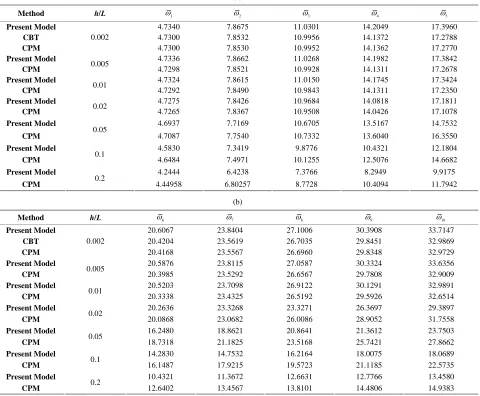
The free vibration validation is performed for the alu- minum beam with material properties given in Table 1. The obtained results are given in Table 5. to Table 7. for beams with different boundary conditions with NE = 35 and the ratio h/L = 0.002 to 0.2. The obtained dimen- sionless frequencies are compared with the previ- ously published results of CBT [28], FSDT [29], TSDT [18], and CPM [16].
For clamped-clamped beam, Table 5(a) shows the following for the first five modes:
1) For h/L = 0.2, the present model results are better than TODT but less than FSDT, and CPM.
2) For h/L less than or equal 0.1, the present model is less than all other theories.
Table 5(b) shows the following for the next five modes (6 - 10):
2 ,
0 10 20 30 40 50 60 70 80 90 100 1.85
1.9 1.95 2 2.05 2.1 2.15 2.2
Number of Elements
Non
D
im
ens
iona
l
F
ir
s
t Nat
ural
F
requa
nc
y
Non Dimensional First Natural Frequancy of Cantilever Aluminum beam
Figure 4. Non-dimensional first natural frequency vs. num-er of elements of cantilevnum-er aluminum beam.
Table 2. Convergence test of the non-dimensional frequency of clamped-clamped aluminum beam with the number of elements.
Mode NE = 10 NE = 15 NE = 20 NE = 25 NE = 30 NE = 35 NE = 40
1 4.7782 4.7502 4.7406 4.7362 4.7338 4.7324 4.7314
2 8.0324 7.9274 7.8918 7.8755 7.8667 7.8615 7.8580
3 11.4368 11.1751 11.0883 11.0489 11.0277 11.0150 11.0068
4 15.0259 14.4920 14.3190 14.2411 14.1994 14.1745 14.1584
5 18.8565 17.8984 17.5937 17.4580 17.3856 17.3424 17.3146
6 22.9619 21.4145 20.9217 20.7043 20.5890 20.5203 20.4762
7 27.2381 25.0601 24.3123 23.9850 23.8122 23.7098 23.6439
8 31.0663 28.8515 27.7749 27.3049 27.0581 26.9122 26.8186
9 32.9891 32.7919 31.3183 30.6690 30.3294 30.1291 30.0011
10 46.6536 32.9891 32.9891 32.9891 32.9891 32.9891 32.9891
11 57.1389 36.8493 34.9500 34.0819 33.6285 33.3621 33.1919
12 65.2975 40.9061 38.6739 37.5477 36.9581 36.6123 36.3920
13 65.3674 44.6623 42.4870 41.0701 40.3205 39.8813 39.6018
14 65.9788 46.6536 46.3727 44.6510 43.7176 43.1701 42.8222
15 73.7684 47.5118 46.6536 46.6536 46.6536 46.4798 46.0535
16 80.8143 57.1388 50.2883 48.2902 47.1511 46.6536 46.6536
17 84.5794 65.9782 54.1445 51.9835 50.6216 49.8114 49.2964
18 87.3015 73.7661 57.1388 55.7200 54.1291 53.1652 52.5511
19 89.2551 80.1672 57.7730 57.1388 57.1388 56.5415 55.8179
20 93.3538 80.1711 60.8863 59.4787 57.6717 57.1388 57.1388
21 94.5830 80.8072 63.0643 63.2219 61.2454 59.9399 59.0968
22 99.0611 87.2829 65.9782 65.9782 64.8425 63.3593 62.3876
23 99.9947 93.3119 73.7659 66.8859 65.9782 65.9782 65.6899
24 104.6635 98.9770 80.8066 70.3684 68.4508 66.7974 65.9782
25 105.3547 102.1423 87.2813 73.5113 72.0505 70.2507 69.0028
1) For h/L equal to or grater than 0.1, the present model is gives more accurate results than all theories by significant values, and this difference increase by in- creasing the mode number.
2) For all modes as the ratio h/L increases the natural frequencies decreases.
Table 6(a) shows the first five modes of Free-Free beam it is clear that:
1) As long as h/L less than or equal to 0.05 the ob- tained results are closed to CBT and CBM theories.
2) For h/L greater than or equal to 0.05 the model re- sults are better than other theories.
Table 6(b) shows the next five modes (6 - 10), for F-F beam as long as h/L less than 0.05 the proposed model gives less accuracy than CPM and CBT theories. For the ratio L/h less than or equal 0.05 the model results are better than CPM theory.
It seen from Table 7(a) for the first five modes of the
S-S beam the proposed model gives results closer to all other theories for all values of h/L.
Table 7(b) shows the modes 6 to 10 for S-S beam it is clear that as long as h/L less than or equal to 0.02, the proposed model gives results closed to other theories. For the ratio h/L greater than or equal 0.05 the model results are better than all other theories with remarkable values.
CASE II: Orthotropic Beam Results a) Model convergences
The convergence of the present model is checked for the orthotropic beam with the material properties given as;
1 2 25,
E E G13 G120.5E2, G230.2E2, 1, and 120.25. A cantilever composite beams with dif- ferent orientation angles [45/-45/45/-45], [30/50/30/50], and [0/90/0/90] with length to height ratio (L/h) is equal to 10, are used. The beam is subjected to uniform distrib- uted load t of intensity 1 N/m. Figure 5 shows the ef- fect of number of element on the normalized transversal
Table 3. (a) Transverse tip deflection of isotropic cantilever beam for different values of applied loads (L/h = 4); (b) Trans- verse tip deflection of isotropic cantilever beam for different values of applied loads (L/h = 10); (c) Transverse tip deflection of isotropic cantilever beam for different values of applied loads (L/h = 20); (d) Transverse tip deflection of isotropic cantile- ver beam for different values of applied loads (L/h = 50); (e) Transverse tip deflection of isotropic cantilever beam for dif- ferent values of applied loads (L/h = 100).
(a)
ft Proposed Model Exact Timoshenko [3] Euler Theory
1 408.8425 408.8400 384
2 817.6849 816.9600 768
3 1.2265e+003 1.2254e+003 1152
4 1.6354e+003 1.6339e+003 1536
5 2.0442e+003 2.0424e+003 1920
6 2.4531e+003 2.4509e+003 2304
7 2.8619e+003 2.8594e+003 2688
8 3.2707e+003 3.2678e+003 3072
9 3.6796e+003 3.6763e+003 3456
10 4.0884e+003 4.0848e+003 3840
(b)
ft Proposed Model Exact Timoshenko [3] Euler Theory
1 1.5151e+004 1.5153e+004 1.5000e+004
2 3.0303e+004 3.0306e+004 3.0000e+004
3 4.5454e+004 4.5456e+004 4.5000e+004
4 6.0606e+004 6.0612e+004 6.0000e+004
5 7.5757e+004 7.5765e+004 7.5000e+004
6 9.0908e+004 9.0918e+004 9.0000e+004
7 1.0606e+004 1.06071e+005 1.0500e+005
8 1.2121e+005 1.21224e+005 1.2000e+005
9 1.3636e+005 1.36377e+005 1.3500e+005
10 1.5151e+005 1.51530e+005 1.5000e+005
(c)
ft Proposed Model Exact Timoshenko [3] Euler Theory
1 2.4055e+005 2.40612e+005 2.4000e+005
2 4.8110e+005 4.81224e+005 4.8000e+005
3 7.2165e+005 7.21836e+005 7.2000e+005
4 9.6220e+005 6.92448e+005 9.6000e+005
5 1.2028e+006 1.203060e+006 1.2000e+005
6 1.4433e+006 1.443672e+006 1.4400e+005
7 1.6839e+006 1.684284e+006 1.6800e+005
8 1.9244e+006 1.924896e+006 1.9200e+005
9 2.1650e+006 2.165508e+006 2.1600e+005
10 2.4055e+006 2.406120e+006 2.4000e+005
(d)
ft Proposed Model Exact Timoshenko [3] Euler Theory
1 9.3760e+006 9378825 9.3750e+006
2 1.8752e+007 18757650 1.8750+007
3 2.8128e+007 28136475 2.8125e+007
4 3.7504e+007 37515300 3.7500e+007
5 4.6880e+007 46894125 4.6875e+007
6 5.6256e+007 56272950 5.6250e+007
7 6.5632e+007 65651775 6.5625e+007
8 7.5008e+007 75030600 7.5000e+007
9 8.4384e+007 84409425 8.4375e+007
[image:11.595.56.539.153.735.2](e)
ft Proposed Model Exact Timoshenko [3] Euler Theory
1 1.4997e+008 1.5002e+008 1.5000e+008
2 2.9994e+008 3.0003e+008 3.0000e+008
3 4.4991e+008 4.5005e+008 4.5000e+008
4 5.9988e+008 6.0006e+008 6.0000e+008
5 7.4985e+008 7.5008e+008 7.5000e+008
6 8.9982e+008 9.0009e+008 9.0000e+008
7 1.0498e+009 1.0501e+009 1.0500e+009
8 1.1998e+009 1.2001e+009 1.2000e+009
9 1.3497e+009 1.3501e+009 1.3500e+009
[image:12.595.56.540.92.240.2]10 1.4997e+009 1.5002e+009 1.5000e+009
Table 4. Transverse tip deflection of isotropic cantilever beam compared with other theories.
L h Proposed Model 5 6 s
k Timoshenko Theory* Timoshenko Theory
5 6 s
k Euler Theory HSDT [15] FE [28] Elasticity Solution
[15]
160 32.8307 32.8355 32.8382 32.6948 32.8376 32.823 32.8741
80 4.1576 4.1572 4.1586 4.0868 4.1587 4.1567 4.17650
40 0.5466 0.5460 0.5467 0.5109 0.5461 0.54588 0.555683
12 12
0.0245 0.0243 0.0246 0.0138 0.02395 0.02393 0.0272414
160 5.6485e004 5.6498e004 5.6498e004 5.6497 56498.3 56444.0 56498.7
80 7.0613e003 7.0629e003 7.0629e004 7.0621 7062.93 7056.3 7063.14
40 1
882.9863 883.1807 883.1890 882.7586 883.188 883.188 883.297
12 23.9581 23.9611 23.9636 23.8345 23.9630 23.9630 23.9959
*
Shear correction factor is: 10 1 12 11 s
k
.
0 10 20 30 40 50 60 70 80 90 100 10
20 30 40 50 60 70 80 90
Number of Elements
N
o
rm
al
iz
e
d
T
ip D
e
fl
ec
ti
on
Tip deflection of Laminated Composite beams
-[45/-45/45/-45]
--[30/50/30/50]
* [0/90/0/90]
Figure 5. Normalized transverse tip deflections vs. number of elements of cantilever composite beams.
tip deflection of beams which is given as:
2 2 4 2 10 t
W wAE h f L , where is the actual transversal deflection. It can be seen that the model predicttions are start to converge at reasonable number of elements for the different beams with different orientation angles.
w
In case of free vibration, the convergences of the natural frequencies of orthotropic beams with the same properties given above in this section are checked for two cases. The dimensionless frequency is defined as:
2 2
i iL EIh
1) First case: Clamped-free beam with different orient- tation angles [45/-45/45/-45], [30/50/30/50], and [0/90/ 0/90]. The obtained results of the dimensionless first natural frequency are shown in Figure 6 for different number of elements.
2) Second Case: Clamped-free and clamped-clamped composite beams with stacking sequences [45/-45/45/ -45], with number of elements changed from 10 to 40. The obtained results are presented in Tables 8 and 9.
It is clear from Figure 6, Tables 8 and 9 that as the number of elements increases the natural frequency de- creases until it reaches a constant value.
b) Static Validation
[image:12.595.56.540.269.414.2]Table 5. (a) Non-dimensional frequency ω of clamped-clamped aluminum beam (Modes: 1 - 5); (b) Non-dimensional fre- quencyωof clamped-clamped aluminum beam (Modes: 6 - 10).
(a)
Method h/L 1 2 3 4 5
Present Model 4.7340 7.8675 11.0301 14.2049 17.3960
CBT 4.7300 7.8532 10.9956 14.1372 17.2788
FSDT 4.7299 7.8529 10.9949 14.1358 17.2765
TSDT 4.7299 7.8529 10.9949 14.1359 17.2766
CPM
0.002
4.7299 7.8529 10.9955 14.1359 17.2766
Present Model 4.7336 7.8662 11.0268 14.1982 17.3842
FSDT 4.7296 7.8516 10.9916 14.1293 17.2650
TSDT 4.7296 7.8516 10.9917 14.1294 17.2652
CPM
0.005
4.7296 7.8516 10.9917 14.1294 17.2651
Present Model 4.7324 7.8615 11.0150 14.1745 17.3424
FSDT 4.7283 7.8468 10.9799 14.1061 17.2244
TSDT 4.7284 7.8569 10.9801 14.1064 17.2249
CPM
0.01
4.7284 7.8469 10.9800 14.1062 17.2246
Present Model 4.7275 7.8426 10.9684 14.0818 17.1811
FSDT 4.7234 7.8281 10.9339 14.0154 17.0675
TSDT 4.7235 7.8283 10.9345 14.0167 17.0696
CPM
0.02
4.7235 7.8281 10.9341 14.0154 17.0679
Present Model 4.6937 7.7169 10.6705 13.5167 14.7532
FSDT 4.6898 7.7035 10.6399 13.4611 16.1586
TSDT 4.6902 7.7052 10.6447 13..4703 16.1754
CPM
0.05
4.6899 7.7035 10.6401 13.4611 16.1590
Present Model 4.5830 7.3419 9.8776 10.4321 12.1804
FSDT 4.5795 7.3312 9.8559 12.1453 14.2323
TSDT
0.1
4.5820 7.3407 9.8810 12.1861 14.3018
(b)
Method h/L 6 7 8 9 10
Present Model 20.6067 23.8404 27.1006 30.3908 33.7147
CBT 20.4204
FSDT 20.4166
TSDT 20.4170
CPM
0.002
20.4168 23.5567 26.6960 29.8348 32.9729
Present Model 20.5876 23.8115 27.0587 30.3324 33.6356
FSDT 20.3983
TSDT 20.3989
CPM
0.005
20.3985 23.5292 26.6567 29.7808 32.9009
Present Model 20.5203 23.7098 26.9122 30.1291 32.9891
FSDT 20.3336
TSDT 20.3350
CPM
0.01
[image:13.595.62.539.126.731.2]Continued
Present Model 20.2636 23.3268 23.3271 26.3697 29.3897
FSDT 20.0866
TSDT 20.0911
CPM
0.02
20.0868 23.0682 26.0086 28.9052 31.7558
Present Model 16.2480 18.8621 20.8641 21.3612 23.7503
FSDT 18.7316
TSDT 18.7573
CPM
0.05
18.7318 21.1825 23.5168 25.7421 27.8662
Present Model 14.2830 14.7532 16.2164 18.0075 18.0689
FSDT 16.1478
TSDT 16.2373
CPM
0.1
16.1487 17.9215 19.5723 21.1185 22.5735
Present Model 10.4321 11.3672 12.6631 12.7766 13.4580
FSDT 12.6357
TSDT 12.8563
CPM
0.2
12.6402 13.4567 13.8101 14.4806 14.9383
Table 6.
![Figure 1. Deformed and un-deformed shape of Timoshenko beam [24].](https://thumb-us.123doks.com/thumbv2/123dok_us/172808.511044/5.595.331.513.614.710/figure-deformed-and-un-deformed-shape-timoshenko-beam.webp)

![Table 8. Convergence Test of the Non-dimensional frequency ω of clamped-free composite beam [45/-45/45/-45] for dif- ferent number of elements](https://thumb-us.123doks.com/thumbv2/123dok_us/172808.511044/16.595.54.539.338.737/table-convergence-dimensional-frequency-clamped-composite-ferent-elements.webp)
![Table 9. Convergence Test of the Non-dimensional frequency ω of clamped-clamped composite beam [45/-45/45/-45] for different number of elements](https://thumb-us.123doks.com/thumbv2/123dok_us/172808.511044/17.595.163.424.510.719/convergence-dimensional-frequency-clamped-clamped-composite-different-elements.webp)
