Munich Personal RePEc Archive
Explaining (in)efficiency in higher
education: a comparison of parametric
and non-parametric analyses to rank
universities
Barra, Cristian and Lagravinese, Raffaele and Zotti, Roberto
University of Salerno - Department of Economics and Statistics,
Roma Tre University - Department of Economics, University of
Salerno - Department of Economics and Statistics
6 October 2015
Online at
https://mpra.ub.uni-muenchen.de/67119/
Explaining (in)efficiency in higher education: a comparison of parametric and
non-parametric analyses to rank universities
Cristian Barra
1Raffaele Lagravinese
2Roberto Zotti
1Abstract
In recent years more and more numerous are the rankings published in the newspapers or technical reports available,
covering many aspects of higher education, but in many cases with very conflicting results between them, due to the fact
that universities‟ performances depend on the set of variables considered and on the methods of analysis employed. The aim
of this study is to rank higher education institutions (HEIs) in Italy, comparing parametric and non-parametric approaches:
we firstly apply a so-called double bootstrap Data Envelopment Analysis (DEA) to generate unbiased coefficients (Simar
and Wilson, 2007) and then a Stochastic Frontier Analysis (SFA), modelling the production set through an output distance
function, applying a within transformation to data as developed by Wang and Ho (2010), to evaluate which determinants
have an impact on universities‟ efficiencies. The findings reveal that, on average and among the macro-areas of the country,
the level of efficiency does not change significantly among estimation methods which, instead, generate different rankings.
This may guide universities‟ managers and policymakers as rankings have a strong impact on academic decision-making
and behaviour, on the structure of the institutions and also on students and graduates recruiters. Variables describing
institution, market place and environment have an important role in explaining (in)efficiency.
Keywords: Universities, Efficiency, Data Envelopment Analysis, Stochastic Frontier Analysis
JEL Codes: I21, I23, C14, C67
1Department of Economics and Statistics, University of Salerno, Via Giovanni Paolo II, 132 - 84084 - Fisciano (SA) – Italy. E-mail: [email protected];
2
1. Introduction
The public budget constraints, due to recent economic crises and the new funding mechanism of the Italian university
system (see Donina et al. 2015 for a description of university governance in Italy), have brought back to the center of both
academic and political debates the assessment of universities‟ performances. In recent years, more and more numerous are
the rankings published in the newspapers or technical reports available, covering many aspects of higher education, but in
many cases with very conflicting results between them (see De Witte and Hudrlikova, 2013 for a detailed discussion on
university rankings and for an alternative methodology to rank universities). Indeed, departments‟ or universities‟
efficiencies depend on the set of variables considered and on the methods of analysis employed. One of the main problems
is, in fact, which variables effectively investigate in order to evaluate the tertiary education system. It is commonly
acknowledged that universities have primarily a double mission: teaching and research1; even though, from the perspective of students, the higher education institutions (HEIs) primary clients, teaching is often considered the main goal, in today's
rapidly-changing political and economic climate, both goals have become increasingly important. Regarding the former
contribution (i.e. teaching), HEIs might contribute to increase the level of human capital (Etzkowitz, 2003); highly skilled
and well-educated individuals are one of the main outputs of universities and at the same time are considered as the ultimate
drive of economic development (Florida et al. 2008). Improvements in the population‟s human capital lead to improvements
in labour, which in turn lead to higher activity rates and lower unemployment rates, thus fostering greater long-term
economic growth in the region. Human capital creation is, indeed, one of the long-term, knowledge-based supply-side
effects according to Florax (1992) and the production of highly educated graduates is likely to cause positive supply-side
effects in the regional economy (Shubert and Kroll, 2014). With regard to the latter task (i.e. research), academic research
quality is universally recognised as influencing market-related university–firm interactions, mainly through contract and
collaborative research (D‟Este and Iammarino, 2010; Laursen et al. 2011) and licensing (Mowery and Ziedonis, 2015).
Universities‟ research activities contribute to the creation of knowledge spillovers leading to an improvement of the
economies (Goldstein and Renault, 2004) and have also impact on the distribution of innovation (Del Barrio-Castro and
García-Quevedo, 2005). In recent years, universities have started being financed according to their level of virtuosity, in
order to achieve higher research performances and to promote academic excellence; “formulas to allocate public funds to higher education institutions are now related to performance indicators such as graduation or completion rates” and “research funding has also increasingly been allocated to specific projects through competitive processes rather than block
grants” (OECD 2008). Both quantitative and qualitative indicators were developed to accurately evaluate the management
of public universities, their productivity in research and teaching and the overall success of their administration; as a
consequence, (public) funds to higher education institutions are now related to performance indicators according to which
evaluate their management and productivity. See Dyson (2000), for a discussion on the need for performance measurement
and strategy.
The statistical and econometric procedures normally used to assess the efficiency in higher education can be classified into
two broad classes: parametric, such as the Stochastic Frontier Approach (SFA), and non-parametric, such as Data
Development Analysis (DEA). However, there is no general consensus about which one has to be adopted to measure
1
3
higher education institutions efficiency, as these two main approaches have not only different features, but also advantages
and disadvantages (Lewin and Lovell 1990)2. DEA does not require, ex-ante, an assumption regarding the functional form of the cost or production function (contrary to SFA) and allows to manage multiple inputs and outputs jointly. Nevertheless,
this method has its drawbacks. Firstly, DEA does not account for stochastic noise in the data. For instance, the results may
be severely biased when measurement errors are present. Secondly, in two stage approaches, the results may be biased due
to the presence of serial correlation (Simar and Wilson, 2007). To obtain unbiased coefficients, a DEA two-stage with a
bootstrap procedure introduced by Simar and Wilson (2007) could be applied through which DEA efficiency scores are
obtained in the first step and then regressed, in the second step, on potential covariates with the use of a bootstrapped
truncated regression. Alternatively, a so-called double-bootstrap method could be also used in which DEA scores are
bootstrapped in the first stage to obtain bias corrected efficiency scores, and then a second stage is performed on the basis of
the bootstrapped-truncated regression. For an application of such methods, see Wolszczak-Derlacz and Parteka (2011), who
examined the efficiency of HEIs in selected European countries, and Curi et al. (2013) who, instead, analysed the efficiency
of the technology transfer operated by the French university system (see also Haelermans and Ruggiero 2013; Coco and
Lagravinese, 2014; Brennan et al. 2014) for an application regarding secondary education). On the other hand SFA requires
an assumption regarding the functional form of the cost or production function. The selection of a function is not a clear-cut
task in higher education as Kraus (2004) pointed out. The most recent literature (Greene, 2005; Wang & Ho, 2010)
emphasized the importance of separating inefficiency and fixed individual effects. Indeed, the efficiency scores may suffer
from the presence of incidental parameters (number of fixed-effect parameters) or time-invariant effects, often
unobservable, that may distort the estimates. Wang and Ho (2010), in order to incorporate heterogeneity in panel data in the
stochastic frontier model, show that first-difference and within transformation can be analytically performed on this model
to remove the fixed individual effects, and thus the estimator is immune to the incidental parameters problem (the latter
being somehow affecting the methods proposed by Greene, 2005). However, to the best of our knowledge, this procedure
has not been frequently used in the higher education environment, yet. Moreover, the presence of a multidimensional nature
of the production (i.e. multiple outputs) may represent a problem when estimating a stochastic production models. To solve
this issue, a distance function approach could been considered (Lovell et al., 1994; Coelli and Perelman, 2000). This
technique is particularly useful when no price information, regarding inputs and outputs, is available (Coelli, 2000). Abbott
and Doucouliagos (2003) estimated output distance functions in order to examine the relationship between competition and
efficiency in Australian and New Zealand universities. Output distance functions have also be estimated by Johnes (2014),
who analysed the effect of efficiency on merger activities in the English higher education sector. So far, to the best of our
knowledge, no papers have investigated the efficiency of Italian HEI combining both non-parametric (DEA) and parametric
2
On one hand, the non-parametric method does not require the building of a theoretical production frontier, but the imposition of certain, a priori, hypotheses about the technology (free-disposability, convexity, constant or variable returns to scale). However, if these assumptions are too weak, the level of inefficiency could be systematically underestimated in small samples, generating inconsistent estimates. Furthermore, this method is very sensitive to the presence of outliers. On the other hand, the parametric method uses a
theoretical analysis to construct the efficient frontier, it‟s not sensitive to extreme values because imposes some assumptions on the error distribution, but must deal with the problem of decomposing the error term. In particular, SFA, proposed by Aigner et al. (1977), Meeusen and Van den Broeck (1977) and Battese and Corra (1977), assumes that the error term is composed by two components with different distributions (see Kumbhakar and Lovell (2000) for analytical details on stochastic frontier analysis). The first component,
regarding the “inefficiency”, is asymmetrically distributed (typically as a semi-normal), while the second component, concerning the
4
approaches (SFA). Therefore, in order to make the estimates more robust and comprehensive, we firstly apply both a
double-bootstrap procedure and a two-stage bootstrap Data Envelopment Analysis (DEA), to generate unbiased coefficients
(Simar and Wilson, 2007), and then we employ a Stochastic Frontier Analysis (SFA), modelling the production set through
an output distance function, using a within transformation to data as developed by Wang and Ho (2010).The first objective
of the paper, is to study the efficiency of Italian HEIs3 using data over the four-years from 2008 to 2011, relying on different criteria of performance indicators, in order to take into account the multiple objectives of higher education institutions, such
as both teaching and research related outcomes. The second contribution of this work, beyond the analyses on HEIs‟
performances already performed in the literature, is bringing new evidence on the importance of comparing the efficiency
estimates derived from various estimation methods (i.e. both parametric and non-parametric techniques) and using the
results from these evaluation processes to rank universities and to provide guidance to university managers and policy
makers. Finally, the third goal of the paper is to analyse exogenous factors which potentially affect university (in)efficiency
such as some institutional details and characteristics of the market place and of the regions where the universities are
located.
The rest of the paper is organized as follows. In Section 2, we present the methodological approaches; Section 3 illustrates
the data, production set and model specification for the empirical analysis; Section 4 contains the main results. Finally,
Section 5 discusses the managerial and policy implications of the main findings with concluding remarks.
2. Empirical Methodology
2.1. Double-bootstrap Data Envelopment Analysis
Until a few years ago, in the DEA standard techniques for estimating what determines the efficiency, the Tobit-estimator
has mainly been applied. However, Simar and Wilson (2007) have emphasized two possible problems stemming from
applying Tobit in this context. Firstly, the results may be biased in the presence of serial correlation between variables at the
two stages; secondly, the efficiency scores may be biased in finite samples. In order to obtain unbiased beta coefficients
with valid confidence intervals, Simar and Wilson (2007) proposed a double bootstrap procedure where DEA scores are
bootstrapped in the first stage to achieve bias corrected inefficiency scores and explained in a bootstrapped truncated
regression with discretionary explanatory variables.
Therefore, in this paper we firstly analyze the technical efficiency4 using a double-bootstrap DEA method (Simar and Wilson, 2007). In particular, we focus on an output-oriented model, following Agasisti and Dal Bianco (2009), who claimed
that “as Italian universities are increasingly concerned with reducing the length of studies, and improving the number of
graduates, in order to compete for public resources, the output-oriented model appears the most suitable to analyse higher
education teaching efficiency”. Moreover, output oriented models seem to be particularly appropriate in the context of
tertiary education according to the fact that the resources used can be considered fixed and that universities cannot
3
See Agasisti (2009), Potì and Reale (2005), Bini and Chiandotto (2003) and Buzzigoli et al. (2010) for a brief review of the university system in Italy.
4
The technical efficiency refers to the capacity of the Decision Making Unit (DMU), given the technology used, to produce the highest level of output from a given combination of inputs, or alternatively, to use the least possible amount of inputs for a given output. Specifically, given that the focus is on the higher education system, technical efficiency means, according to Abbott and Doucouliagos
(2003), that “the technically efficient university is not able to deliver more teaching plus research output (without reducing quality) given
5
influence, at least in the short run, the human, financial and physical capital available (Bonaccorsi et al. 2006). Therefore,
we present an output-oriented model. Suppose that a Decision Making Unit (DMU) – in our case the university - can be
characterized by a technological set defined as:
*(𝑥 𝑦) 𝑥 𝑛 𝑝 𝑜 𝑦+ (1)
Where 𝑥 represents a vector of inputs and 𝑦 the vector of outputs.
Specifically, we use a Farrell/Debreu output-oriented technical efficiency measure such as:
(𝑥 𝑦) * (𝑥 𝑦) + (2)
where measures the maximum possible increase in output , given that inputs remain constant.
We assume variable return to scale (VRS); the DEA-VRS is probably the most reliable in our case as suggested by Agasisti
(2011), who argued that the assumption of constant return to scale is restrictive because it is reasonable “that the dimension
(number of students, amount of resources, etc.) plays a major role in affecting the efficiency” especially if we consider, as
we do, the DMUs trying to achieve pre-determinate outputs, given certain inputs.
Thus, at the first stage, we estimate equation (1) through the following linear programming:
̂ {(𝑥 𝑦) ∑ 𝑦 𝑦
∑ 𝑦 𝑥
} 𝑛 (3)
where 𝑦 is a vector of constants
In the second stage, we use the DEA efficiency scores (calculated in the first step) as dependent variable (̂) regressing
them on potential exogenous environmental variables (𝑧):
̂ 𝑧 𝑛 (4)
where is a statistical noise.
A problem may arise due to the fact that true DEA scores, obtained in the first step, are unobserved and replaced by
previously estimates ̂, which, in turn, are serially correlated in a unknown way; moreover, the disturbance error is
correlated with 𝑧 as a consequence of the fact that inputs and outputs can be correlated with the environmental variables.
To solve these issues, we use a consistent bootstrap approximation of the efficiency distribution, in which DEA scores are
bootstrapped in the first stage, to obtain bias corrected efficiency scores; then, in the second stage, in order to analyse the
dependency of the efficiency on a set of potential covariates, we apply a consistent bootstrap-truncated regression to
consistently estimate the parameters by using maximum likelihood and for inference. We also use a two-stage DEA analysis
where the efficiency scores are obtained in the first step and then they are regressed, in the second stage, on potential
covariates, using again a bootstrap-truncated regression.
6
efficiency scores, we utilize Wilson‟s FEAR 1.15 software (2008) which is freely available online, and the truncated
regression models were then performed in STATA 12 software.
2.2. A stochastic education distance frontier
The analysis explores also the Stochastic Frontier Analysis, because it offers useful information on the underlying education
production process, as well as information on the extent of inefficiency. Nowadays, the most widely applied SFA technique
is the model proposed by Battese and Coelli (1995), to measure technical efficiency across production units. Intuitively,
technical efficiency is a measure of the extent to which an institution efficiently allocates the physical inputs at its disposal
for a given level of output. The presence of a multidimensional nature of the production (i.e. multiple outputs) may
represent a problem when estimating a stochastic production models. To solve this issue a distance function approach has
been considered (Lovell et al. 1994; Coelli and Perelman, 2000). Moreover, this technique is particularly useful when no
price information regarding inputs and outputs is available (Coelli, 2000). Specifically, and following Abbott and
Doucouliagos (2003) and Johnes (2014), we choose to model the production set through an output distance function in a
panel context. Moreover, on a methodological ground, the most recent literature, which deals with panel data, emphasized
the importance of separating inefficiency and fixed individual effects. Indeed, the efficiency scores may suffer from the
presence of incidental parameters (number of fixed-effect parameters) or time-invariant effects, often unobservable, that
may distort the estimates (Greene, 2005; Wang and Ho, 2010). For instance, students‟ or researchers‟ (average) innate
abilities may be an important determinant of their individual academic achievements and thus account for an important
share of the heterogeneity in data when evaluating the efficiency of the institution in which they are studying or working. As
Wang and Ho (2010) have underlined: “(…) stochastic frontier models do not distinguish between unobserved individual
heterogeneity and inefficiency”, forcing “all time-invariant individual heterogeneity into the estimated inefficiency”. In order to deal with this problem and to estimate the technical efficiency, we apply a within transformation to data as
developed by Wang and Ho (2010). By this transformation, the sample mean of each panel is subtracted from every
observation in the panel, removing time-invariant individual effects from the model. Following the notation in Wang and Ho
(2010), the transformation employed to our model is:
𝑤 . ( /𝑇) ∑ 𝑤 𝑡 𝑤 𝑡. 𝑤 𝑡− 𝑤 . 𝑇
𝑡
(5)
The stacked vector of 𝑤 𝑡. for a given i is:
𝑤̃ . (𝑤 . 𝑤 2. 𝑤 𝑇.)′ (6)
For simplicity, hereafter in our formulation does not include a subscript t. The baseline model associated to distance
function after the transformation can be written as:
7
where 𝑦 ̃ represent the conventional outputs, 𝑥 ̃ denote the conventional inputs and ̃ denotes the disturbance term.
Following a common practice, we now assume a functional form a‟ la Cobb-Douglas for the output distance function:
𝑙𝑛𝐷̃ .𝑜 ∑ 𝛼̃𝑚 𝑚
𝑙𝑛𝑦̃𝑚 . ∑ ̃𝑘 𝐾
𝑘
𝑙𝑛𝑥̃𝑘 . 𝑣̃
(8)
By a within transformation, 𝛼 (intercept that changes over time according to a linear trend with unit-specific time-variation
coefficients and that represents time-invariant effects) disappears from our specification. Normalizing5 by 𝑦̃, that guarantees the linear homogeneity of degree 1 in outputs (∑𝑚 𝛼̃𝑚 ) as suggested by Lovell et al. (1994), the output
oriented distance function becomes:
𝑙𝑛 (𝐷̃ .𝑜
𝑦̃ .) ∑ 𝛼̃𝑚𝑙𝑛𝑦̃𝑚 . ∗
𝑚
∑ ̃𝑘
𝐾
𝑘
𝑙𝑛𝑥̃𝑘 . 𝑣̃
(9)
where 𝑦̃𝑚 .∗ 𝑦̃𝑚 ./𝑦̃ ., 𝑦̃ .∗ 𝑦̃ ./𝑦̃ . and thus 𝑦̃ . . In addition, the time dummies are also taken into account in order to
capture exogenous or business cycle effects that can influence the production process of the decision-making units (i.e.
universities). It‟s obvious that 𝑙𝑛(𝐷̃ .𝑜) is not observable. Then, in order to solve this problem, we can re-written 𝑙𝑛(𝐷̃ .𝑜/
𝑦̃ .) 𝑙𝑛(𝐷̃ .𝑜) - 𝑙𝑛(𝑦̃. ). Thus, we transfer 𝑙𝑛(𝐷̃ .𝑜) to the residuals, i.e. on the right and side of the equation (9), and using
−𝑙𝑛(𝑦̃ .) as dependent variable (Coelli and Perelman, 2000). In our case, we follow Paul et al. (2000), i.e. imposing 𝑙𝑛(𝑦̃). The equation (9) thus becomes:
𝑙𝑛(𝑦̃ .) ∑ 𝛼̃𝑚 𝑚
ln (𝑦̃𝑦̃𝑚 .∗
. ) ∑ ̃𝑘 𝐾
𝑘
𝑙𝑛𝑥̃𝑘 . 𝑣̃ − ̃
(10)
where ̃terms stands for inefficiency component, obtained from the truncation to zero of the distribution (𝑚̃ 𝜎̃𝑢2), where
𝑚̃ 𝜇̃ 𝑧̃ ̃, 𝜇̃ denoting the location parameter, 𝑧̃ a vector of determinants of (technical) efficiency and ̃ is a vector of unknown coefficients; indeed 𝑣̃ denotes the vector of random variables assumed to be i.i.d. ( 𝜎̃𝑣2) and independent of the
̃. In other words, the inefficiency of university is assumed to systematically vary with respect to some determinants (see Section 3 below for more detail on production set). Time dummies are also included in order to capture the influence of exogenous factors. In this analysis, we do not impose the “scaling property” (for more details see Wang and Schmidt (2002) and Alvarez et al. (2006)) because produces estimation problems in our model. In fact, as suggested in literature (see for
instance Wang and Ho, 2010), whether the scaling property holds in the data is ultimately an empirical question. In other
words, we assume changes not only in scale but also in the shape of the inefficiency distribution.
5
8
Specifically, a Cobb-Douglas6 production function7 is preferred in this paper firstly because it allows us to overcome the multicollinearity problem and biases in the coefficients associated to estimate a few number of parameters with respect to
the translog function and secondly because it‟s more comparable with a non-parametric approach.
The validity of the heteroschedastic assumption is tested using a Likelihood Ratio (LR) test which allows us to identify the
fit of the model and to confirm the imposition of some determinants in the inefficiency term. All coefficients of the output
distance function, estimated through a maximum likelihood estimator (MLE), and technical efficiency are obtained using
the STATA 12 software.
3. Data, the production set and model specification
3.1. Selected inputs and outputs
The dataset refers to Italian public universities over the four years period 2008-2011 and it has been constructed using
data which are publicly available on the National Committee for the Evaluation of the University System (CNVSU)
website8. We exclude all private sector universities, due to the absence of comparable data on academic research variables;
this leaves us with a sample of 53 universities9, each of which yields data over the four year period, so we have a total of 212 observations.
Referring to the literature on this subject, the production technology is specified, with four inputs: 1 – number of academic
staff; 2 - percentage of enrolments with a score higher the 9/10 in secondary school; 3 – the percentage of enrolments who
attended a lyceum; 4 - total number of students. More specifically, the first input is the number of academic staff
(ACADSTAFF). It is a measure of a human capital input and it aims to capture the human resources used by the universities
for teaching activities (see Johnes, 2014; Agasisti and Dal Bianco, 2009)10. The second and third inputs are the percentage of enrolments with a score higher the 9/10 in secondary school (ENRHSG) and the percentage of enrolments who attended a
6
With stochastic frontier analysis, a frontier is estimated on the relation between inputs and outputs. This can, for example, be a linear function, a quadratic function or a Translog function. This paper uses a Cobb-Douglas function. However, there is no general consensus about which one is to be adopted in the higher education environment (for a discussion on the different function forms, see Agasisti and Johnes, 2009). The assumptions behind the use of Cobb–Douglas production functions are plausible in view of the theoretical model which describes the human capital formation in the university system. It allows us to overcome the multicollinearity problem associated to estimate a few number of parameters with respect to the translog function; therefore it is less susceptible to multicollinearity and degrees of freedom problems than the translog function (see Laureti, 2008, who uses a Cobb-Douglas function in order to model exogenous variables in human capital formation).
7
Therefore, all inputs and outputs are in log level. 8
Specifically, data have been collected by the Italian Ministry of Education, Universities and Research Statistical Office. 9
Which is very representative of the higher education system in Italy, corresponding to almost 90% of the total number of public universities in the country (we are not able to cover the complete population of universities due to missing information on some of the variables used in the analysis).
10
The variable ACADSTAFF indicates the number of total academic staff adjusting for the respective academic position. Specifically, the
academic staff has been disentangled in four categories, namely professors, associate professors, assistant professors and lectures. In order to take into account this categorization, we assign weights to each category according to their salary and to the amount of institutional, educational and research duties the academic staff has to deal with (see Madden et al. 1997) and assuming that a professor is expected to produce more research and teaching work than an associate professors and so on (see Carrington et al. 2005). We follow Halkos et al. (2012) where professors are assigned with 1, associate professors with 0.75, assistant professors with 0.5 and lecturers with 0.25. They basically choose weights so that the distance between two ranks is 1/4=0.25. Thus, we use the following aggregate measure of human capital input: Academic Staff (ACADSTAFF)=1*professors+0.75*associate professors+0.50* assistant professors +0.25* lectures.
9
lyceum11(ENRLYC), with respect to the total number of students enrolled. Indeed, among the inputs that are commonly
known to have effects on students‟ performances there is the quality of the students on arrival at university. There is strong evidence that the type of secondary high school and pre-university academic achievement are important determinants of the
students‟ performances (Boero et al. 2001; Smith and Naylor 2001; Arulampalam et al. 2004; Lassibille 2011). The underlying theory is that ability of students lowers their educational costs and increases their motivation (DesJardins et al.
2002). Thus these two inputs aim to capture the quality of students on arrival at university (i.e. proxies of the knowledge
and skills of students when entering tertiary education)12. The fourth and last input is the total number of students (STUD) in order to measure the quantity of undergraduates in each university13 (Agasisti and Dal Bianco, 2009).
Moving to the output side, two measures of outputs are included in the model reflecting the teaching and research functions
of HEIs: 1 – number of graduates weighted by their degree classification; 2 – research grants. According to Catalano et al.
(1993) “the task assigned to universities is to produce graduates with the utilization and the combination of different
resources” and Madden et al. (1997) used the number of graduates under the hypothesis that the higher is the number of
graduates the higher is the quality of teaching14. Also Worthington and Lee (2008) considered the number of undergraduate
degrees awarded an obvious measure of output for any university. Thus, the first output considered in the analysis is the
number of graduates weighted by their degree classification15 (GRADMARKS), in order to capture both the quantity and the
quality of teaching (see also Johnes, 1996; Johnes 2006; Madden et al. 1997). As the focus of the paper is on both teaching
and research, we include as an output also a measure of research performances of the universities. Academic research is the
most controversial output and different proxies have been used in the literature such as bibliometric indicators and peer
review (De Groot et al. 1991) and weighted indexes of publications (Athanassoupoulos and Shale, 1997; Johnes and Johnes,
1993; Tyagi et al. 2009; Johnes and Yu, 2008; Halkos et al. 2012). Information on the number of publications is not
11
For the readers who are not familiar with the characteristics of the Italian secondary school system, in Italy, students before entering at University attend five years of high school. This secondary school is divided in two types: a) vocational schools are higher-level learning institutions which are specialized in providing students with the vocational education and technical skills they need in order to perform the tasks of a particular job; b) non-vocational secondary schools, instead, are more academic oriented and are specialized in providing the students the skills needed in order to enroll in the university. The latter, in Italy, is also called Lyceum. So, basically, the variable percentage of enrolments who attended a lyceum (ENRLYC) is the percentage of students who attend a Lyceum (i.e. secondary
schools who prepare students to the university). In other words, supported by the literature on the education system using Italian data, the
idea is that the higher is the percentage of enrolments who come from “Lyceum” the higher is the quality of the university.
12
We look at the correlation between ENRHSG and ENRLYC. Both Pearson and Spearman correlation coefficients are positive
and statistically significant, but their magnitude does not suggest to have concerns regarding multicollinearity problems. In other words, we believe these variables control for two different aspects of pre-enrollment characteristics such as the quality of the secondary school attended (secondary school track chosen) and the secondary high school grade (a measure of academic preparedness). Correlation coefficients are not presented in the paper due to space constraints and available on request.
13
The second and third inputs (ENRHSG and ENRLYC) are used as percentages in order to avoid a double counting problem due
to presence of the total number of students (STUD) among the inputs. In this way we are able to measure the quantity of undergraduates in each university (through STUD) and include in the production process also two important information regarding the quality of the students enrolled in each university (ENRHSG and ENRLYC).
14
The liability of this measure is still not clear in the literature. See Kao and Hung (2008) and Abbott and Doucouliagos (2003) for a discussion.
15
For the readers who are not familiar with the characteristics of the Italian higher education system, in Italy students can graduate obtaining marks from 66 to 110 with distinction. This grade is calculated mainly according to the average grades students have obtained in the exams; then a certain number of points is added after the final dissertation has been graded. In order to weight the graduates according to their degree marks, we apply the following procedure: GRADMARKS =1* graduates with marks between 106 and 110 with
distinction +0.75*graduates with marks between 101 and 105 + 0.5*graduates with marks between 91 and 100+0.25*graduates with marks between 66 and 90. The weights have been chosen so that the distance between two ranks is ⁄ . . For robustness, we also further test how alternative weights given to the GRADMARKS variable, to avoid a severe discounting of the students earning less than top
marks, would change the results as follows: GRADMARKS=1*graduates with marks between 106 and 110 with distinction+0.75*graduates
10
available to us, thus we use research grants (RES) as a second output and as a proxy of research outputs (see Abbott and
Doucouliagos, 2003; Agasisti and Johnes, 2010; Kao and Hung, 2008; Agasisti and Johnes, 2009; Agasisti et al. 2012;
Worthington and Lee, 2008). According to Agasisti and Johnes (2010), “Grants represent a measure of the market value of
research done, and so provides a neat conflation of the quantity and quality of research effort. They also provide a measure
of research output that is less retrospective than bibliometric analyses”. Research grants reflect the market value of the
research conducted and can, therefore, be considered as a proxy for output (Cave et al., 1991; Tomkins and Green, 1988).
Specifically, in our case, it represents the amount that the government is willing to pay the universities for the research they
produce. We are aware that the use of grant income might raise some problems related to the presence of a lag between the
publication of research output and the generation of that research; however, according to Hashimoto and Haneda (2008) this
is more important when using citation counts or number of patents than research income measure. Moreover, according to
Johnes (2014), the use of research grants as an output “is also an attractive measure of research in that it provides an up
-to-date picture of research activity and output in the current academic year”. Thus, also considering that there are no clear
criteria for deciding on the appropriate length of lag (Emrouznejad and Thanassoulis, 200516) and following Johnes (2014), we use a static model in our analysis. See also Frey and Rost (2010) for a discussion on the appropriate measures of
research quality and quantity.
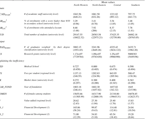
When looking at the descriptive statistics (Table 1 below), it is interesting to notice that, considering the four geographical
areas in which we have aggregated the universities and taking into account the inputs, the Southern area shows the lowest
number of academic staff and, interestingly, the highest percentage of enrollments with a score higher than 9/10 in
secondary school. The number of students is, instead, more stable across the areas. Considering the performances (output
side) by geographical areas, the North-Central areas outperform the Southern area both considering the number of graduates
weighted by their degree marks and the grants received for the research activities.
[Table 1] around here
3.2. Factors affecting university (in)efficiency
At this stage, DEA and SFA scores are linked with several factors, related to the institutional details and some
characteristics of the marketplace and the environment where the institutions are located, that may influence universities‟
performances. These factors are modelled as variables, which directly influence the variability of the inefficiency term. In
other words, they affect the efficiency with which inputs are converted into outputs. The model to be estimated takes on the
following form:
𝑡 𝛼 𝐷 𝑡 2 𝑡 𝑡 𝑡2 𝐷 𝑡 𝑡 𝑡 𝐷 𝑡
𝑇 𝑡
(11)
where refers to single university, the region where it is located and denotes time period; 𝐷 is a dummy variable
equalling 1 if the university has a Medical Faculty and 0 otherwise; it has been included in order to take into account the
16
11
specificity of faculty composition (see Kempkes and Pohl, 2010, for a similar approach); represents the fees per
student calculated as the ratio of the amount of income received by the university from the fees pays by the students over
the total number of students, in order to take into account the services offered by the institution17; is the market share measured as the ratio between the number of enrolments at university and the total number of enrolments in the
universities located in the same region, included for capturing the potential effects due to the presence of more
concentration or competition between universities; 𝐷 is the year of foundation of the university as a proxy for
the level of tradition of a given HEIs as it is often perceived that HEIs with a longer tradition have a better reputation, b ut it
could also be the case that younger HEIs have more flexible and modern structures, assuring a more efficient performance;
is the number of females among students in order to test the relation between the gender composition of the students and universities‟ efficiency scores; is the added value per capita corresponding to the difference between the
production value of goods and services created by individual productive branches and the value of the intermediate goods
and services consumed by them, with the aim of controlling for the growth of the economic system in terms of new goods
and services made available to the community for final use18; 𝐷 represents the financial development measured as
aggregate private credits relative to GDP (as robustness we also use aggregate private deposits relative to GDP). Finally,
𝑇 denotes dummies trend capturing the presence of exogenous effects on the phenomenon analysed, while is the vector of error terms. We measure 𝐷 𝐷 and at university level, while and 𝐷 are
instead measured at regional level. See Table 2 below, for more details on the specification of inputs, outputs and
exogenous factors.
[Table 2] around here
4. Results
4.1. Efficiency scores
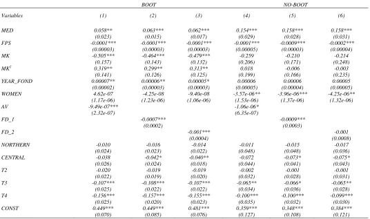
Table 3, below, presents the estimated parameters from the DEA analysis as described in Section 2.1. The dependent
variable is Farrell's bias corrected efficiency score of the i-th university derived from DEA estimates. Table 3 reports both
17
More specifically, it corresponds to the fees income received from undergraduates students. For the readers who are not familiar with the Italian higher education system, Italian universities are free to set their own student fees, even though their amount is partially constrained by a national regulation and there is a legal minimum fee for enrolment and maximum level for student contributions to costs
and services, which cannot exceed 20% of state funding. Usually, the level of these fees is quite low (around 1,200€ per year) and covers only a small fraction of the real cost per student; nevertheless, this source of income gained importance in the last years (to contrast the reduction of public funds) and now represents, on average, 15% of the total university budget. Fees do not depend on the subject studied and are usually set according to the ISEE index which is an instrument used to measure the actual property and income position of citizens that apply for social services under favourable terms and is determined by combining and evaluating three elements: income, assets and composition of the household. To calculate the ISEE index to the fiscal year at time t, gross income to all members of the household at time t as reported at time t+1 is used, along with the composition of the self-reported information about the value of
household‟s assets in real estate at the end of t year, cadastral certificates or other documents regarding real property, etc. Therefore, fees are paid by students proportionally to the amount declared in the ISEE. Therefore, in some cases, students are exempted from paying tuition fees depending on their financial situation and also on their academic performances. It has also to be said that however, student
fees represent just a part of universities‟ income. For the remaining part, universities are mostly funded directly by the Ministry of Education, which also has the major responsibility for regulating higher education (for example, staff salaries, rules to activate courses).
18
12
standard efficiencies (No boot – i.e. DEA scores are not bootstrapped) and bias corrected efficiencies (Boot – i.e. DEA
scores are bootstrapped) as well as the bias found in our estimation (Bias).
[Table 3] around here
First of all, our evidence suggests the importance of using a double-bootstrapped DEA approach; indeed, the main results
are confirmed but a strong bias is found in our estimation, meaning that the efficiency scores calculated without bootstrap
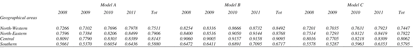
might be over-estimated. Examination of Table 3, shows the presence of some geographical effects (by macro-areas) with
institutions in the Central-North area (North-Western, North-Eastern and Central) outperforming those in the Southern area;
this is customary for the literature on Italian universities (see, e.g., Agasisti and Dal Bianco, 2009). Taking the average
across years into consideration (last three columns of Table 3), the estimated gap of efficiency scores is in the order of
slightly less than 10% between the Central-North regions of the country and the Southern one; for instance the average
efficiency of the North-Eastern area is estimated around 72% - in other words, the output expected can be expanded by
around 28% using the same amount of inputs. Instead, the Southern area is around 64%, thus their inputs can be used
more efficiently for producing around three/fourth more outputs. Table 4 below, instead, presents the estimated
parameters of the stochastic education distance frontier presented in Section 2.2.; from a methodological perspective, the
null hypothesis that there is no heteroscedasticity in the error term has been tested and rejected, at 1% significance level,
using a Likelihood Ratio Test (LR), giving credit to the use of some exogenous variables, according to which the
inefficiency term is allowed to change. In other words, the validity of heteroscedastic assumption has been confirmed,
leading to the significance of the inefficiency term. The coefficients show that all the inputs variables have a positive and
statistically significant effects on the various outcomes of the universities19. The geographical effects (by macro-areas) already found are confirmed with regions in the Central-North area still outperforming those in the Southern area.
[Table 4] around here
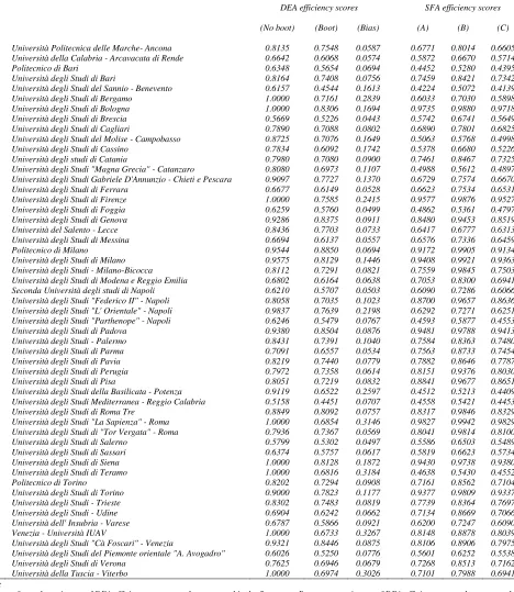
Table 5, below, summarizes the efficiency estimates for each university in the sample. When looking at the non-parametric
estimates (DEA efficiency scores), the mean efficiency of all universities is 0.6882 (to confirm the importance of obtaining
the bootstrapped efficiency scores, the mean efficiency of all universities is 0.8056 without the bootstrapping procedure
created by Simar and Wilson, 2007), with slightly more than 50% of the universities having a level of efficiency
over the sample mean. Again, it is clear than the universities located in the Central-North area perform better than those in
the Southern area (75% of the universities with a level of efficiency over the sample mean are located in the Central-North
area). Still taking into account the geographical effects, some information could be gained also when we consider
the big city areas where many universities are located. For instance, the Rome area (where Roma La Sapienza, Roma Tor
Vergata and Roma Tre are located), is particularly efficient with an average efficiency of 0.7437 among all the years.
The Milan area (where Milano University, Milano Bicocca and Milano Politecnico are located) also shows good
performances with an average of 0.8090 among all the years. Finally the Naples area (where Napoli Federico II, Napoli II,
19
13
Napoli L‟Orientale and Napoli Parthenope are located), shows lower performances with an average of 0.6465 among all the
years.
[Table 5] around here
When looking, instead, at the parametric estimates (SFA efficiency scores), it is even more clear than the universities
located in the Central-North area perform better than those in the Southern area as now around 86% of the universities with
a level of efficiency over the sample mean are located in the Central-North area (the mean efficiency of all universities is
0.7023, considering Model A in Table 5). When we consider the big city areas where many universities are located, the
Rome area (where Roma La Sapienza, Roma Tor Vergata and Roma Tre are located), is particularly efficient with an
average efficiency of 0.8728 among all the years. The Milan area (where Milano University, Milano Bicocca and Milano
Politecnico are located) also shows good performances with an average of 0.8713 among all the years. Finally the Naples
area (where Napoli Federico II, Napoli II, Napoli L‟Orientale and Napoli Parthenope are located), shows lower
performances with an average of 0.6418 among all the years.
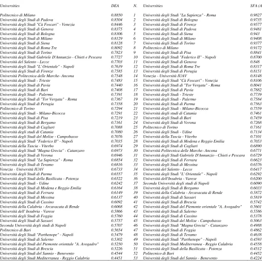
The main difference, among the two estimation methods employed in the paper, regards the university rankings (seeTable 6,
below). Indeed, looking for instance at the universities ranked in the first 10 position, 8 of them - Università degli Studi "Cà
Foscari" – Venezia, Università degli Studi di Genova, Università degli Studi di Roma Tre, Università degli Studi Gabriele
D'Annunzio - Chieti e Pescara (when using DEA), and - Università degli Studi "La Sapienza" – Roma, Università degli
Studi di Firenze, Università degli Studi di Pisa, Università degli Studi "Federico II" – Napoli (when using SFA), are present
only in one of the rankings; instead, only few of them (Politecnico di Milano, Università degli Studi di Padova, Università
degli Studi di Bologna, Università degli Studi di Milano, Università degli Studi di Siena, Università degli Studi di Torino)
are present in both rankings. Among them, only one of the university (Università degli Studi di Torino) assumes the same
position (6th). While, all the other universities which are present in both rankings, are positioned differently.
[Table 6] around here
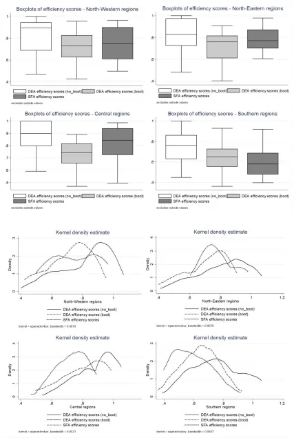
Boxplots and Kernel distributions of efficiency scores (pooling all years) are presented in Figure 1 below. Differences
between efficiencies of universities not only in the mean, but also in the distribution is shown through the boxplots;
considering the Kernel distributions, the universities are more efficient, the closer they come to the value of one.
North-Central regions of the country are characterized by a skewed distribution with more concentration in the direction of more
efficient units; moreover, comparing biased (non-bootstrapped) and unbiased (bootstrapped) efficiency scores, it‟s clear that
the distribution of the latter one are slightly on the left indicating lower level of efficiency scores.
[Figure 1] around here
4.2. (In)efficiency score determinants
When considering the exogenous factors included in the analysis, our findings show that the variables used to control for the
different competitive environment in which institutions are located, have an important role in describing the inefficiency
14
regression parameter indicates that, ceteris paribus, an increase in a variable corresponds to higher inefficiency (lower
efficiency), while a negative sign of estimated parameter indicates lower inefficiency (greater efficiency).
[Table 7] around here
Specifically, we found a positive and significant coefficient, which indicates a lower efficiency, for universities with regards
to the medical faculty (MED); as already specified by Curi et al. (2012), the empirical evidence on whether the presence of
medical schools make universities more or less efficient is controversial, and the “differences in results might be due to the
different production process characterizations in the different models”. Our findings are consistent with the studies by
Thursby and Kemp (2002), Anderson et al. (2007) and Chapple et al. (2005) who show that the presence of a medical
school reduces the efficiency level, probably due to the heavy service commitments of medical schools or to differences in
the health product market20. We also find a negative and statistically significant coefficient on the fees per student variable (FPS); this indicates that the higher levels of fees per capita are associated with higher levels of universities‟
efficiency. This finding is also consistent with the interpretation that when market forces operate, there are benefits for
HEIs‟ efficiency – an analogous finding about the positive association between efficiency and fees of Italian universities is in Agasisti and Wolszczak-Derlacz (2014)21. Moreover, inefficiency has a U-shaped relationship with respect to the measure of market competition (MK), showing a negative and statistically significant relationship between
inefficiency and market share while, instead, a positive and statistically significant relationship between inefficiency and
(squared) market share has been found (specifically when bootstrapped efficiency scores are estimated, see Column 1, 2
and 3, Table 7). In other words, the increase in concentration does not lead to a linear change in efficiency; at some
point, the effect becomes positive, and the quadratic shape means that the inefficiency of HEIs with respect to the measure
of market concentration is increasing as concentration increases (i.e. universities are less efficient), and the results can be
due to the finishing incentives in becoming efficient when concentration arises indeed. Overall, these findings suggest that
differences in performances might be due to the market structure of higher education, in the direction that a more
competitive environment could lead to higher efficiency. The estimation results reveal that the coefficient associated with
the presence of female students (WOMEN) is, in general, negative and statistically significant, meaning that the higher is
the share of females among the students the higher is the efficiency of the universities (specifically when not-bootstrapped
efficiency scores are estimated, see Column 4, 5 and 6, Table 7). A negative and statistically significant coefficient has been
found on the variable value-added (AV), and on the financial progress variables (FD_1 and FD_2), which means that
operating in more economically developed areas is associated, on average, with higher efficiency. Finally, results
show that younger universities (YEAR_FOND) are less efficient. The importance of using a double bootstrapped approach
is evident not only when looking at the universities‟ efficiency scores (see Table 5 above), but also when the (in)efficiency
score determinants are taken into account (see Table 7, Columns 1, 2 and 3 vs Column 4, 5 and 6). See for instance the
reduction in the magnitude of the coefficient related to the presence of a Medical school (MED) and the measure of the
market share (MK) which become statistically significant when the bootstrap is performed.
20
For a different perspective, see Siegel et al. (2008) who, instead, show that the presence of a medical school does have a positive and
statistically significant impact on universities‟ efficiencies. 21
15
[Table 8] around here
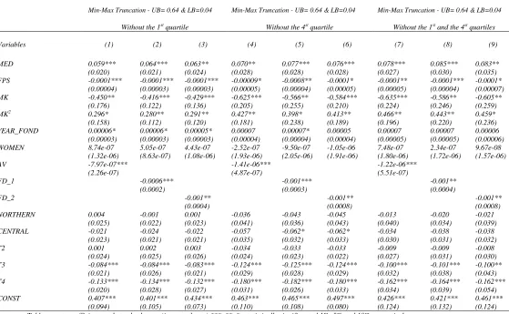
Regarding the two stage DEA approach, for robustness, we also further investigate whether the distribution of the efficiency
affect the estimates, in the second step. Indeed, we divide universities in quartiles, and repeat the analysis firstly removing
from the sample those universities with an efficiency score in the first quartile - taking out the less efficient universities –
(see Table 8, Columns 1, 2, 3), then those with efficiencies scores in the last quartiles - taking out the more efficient
universities – (see Table 8, Columns 4, 6, 7) and ultimately taking out both (see Table 8, Columns 7, 8, 9). Results are
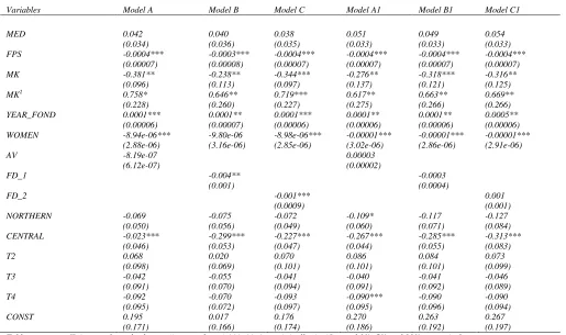
confirmed. Finally, Table 9 shows the determinants of inefficiency scores when the SFA approach has been used. When
comparing non-parametric and parametric methods, (see Tables 7 and 9), results do not show important differences, apart
from the presence of a Medical school (MED), which is still positive (meaning a lower efficiency for universities with
medical school) but it is not statistically significant anymore.
[Table 9] around here
5. Conclusions
The main aims of this research were to evaluate the efficiency of Italian universities, and to investigate some exogenous
characteristics affecting their efficiency, underlining the importance of comparing the efficiency estimates derived from
various estimation methods, in order to rank universities. In order to reach these goals, both parametric and non-parametric
techniques have been applied; we firstly apply both a double-bootstrap procedure and a two-stage bootstrap Data
Envelopment Analysis (DEA), to generate unbiased coefficients (Simar and Wilson, 2007) and then a Stochastic Frontier
Analysis (SFA), modelling the production set through an output distance function, applying a within transformation to data
as developed by Wang and Ho (2010), to evaluate which determinants have an impact on universities‟ efficiencies.
Results reveal, as customary for the literature on Italian universities, the presence of some geographical effects with
institutions located in the Central-North area showing higher efficiency scores than those in the Southern area, with both the
empirical approaches. More specifically, when apply a bootstrapping method in contrast to straightforward application of
DEA (in order to investigate the sensibility of efficiency scores relative to the sampling variations of the estimated frontier
and thus obtain bias corrected efficiency estimates) the empirical evidence shows that the efficiency scores calculated
without bootstrap might be over-estimated suggesting the importance of using a bootstrapped DEA approach. On average,
the level of efficiency does not change very much among estimation methods even though the universities are ranked
differently. For instance, looking at the universities ranked in the first 10 position, 8 of them are present only in one of the
rankings; instead, only few of them are present in both. Moreover, among them, only one of the university assumes the
same position, while all the other universities which are present in both rankings, are positioned differently. In other words,
the methods of analysis employed do matter when ranking universities.
At the second stage of our analysis, we linked the technical efficiency scores of single HEIs with variables describing their
location, the institution, year of foundation and some characteristics of the marketplace; indeed, the results show that
inefficiency is U-shaped relationship with respect to the measure of market competition in favor of a more competitive
16
inefficiency as well as that the higher is the value added per capita the lower is the technical level of inefficiency. The
findings provide a clue towards the expansion of pro-competitive policies in the Italian higher education sector, consistently
with the interpretation that when market forces operate, there are benefits for university efficiency.
This exercise provide guidance to university managers and policymakers, warning them that the estimates of the level of
efficiency could vary by estimation methods and, more importantly, that the ranking of universities may change; this is
particularly important considering that rankings have a strong impact on academic decision-making and behaviour, and on
the structure of the institutions (Hazelkorn, 2007), that higher education institutions are focusing on the criteria with the
highest impact on the ranking (Tofallis 2012), and that also students and graduates recruiters follow the hierarchy of
institutions (see Clarke, 2007; Harvey, 2008). In other words, as both human and financial resources might depend on how
the university are positioned in such rankings, it is useful to providing further light on the delicate processes of evaluating
17
References
Abbot, M. and Doucouliagos, C. (2003). The efficiency of Australian universities: a data envelopment analysis. Economics of Education Review, 22, 89-97.
Agasisti, T. (2009). Market forces and competition in university systems: theoretical reflections and empirical evidence from Italy. International Review of Applied Economics, 23 (4), 463–483.
Agasisti, T. (2011). Performances and spending efficiency in Higher Education: a European comparison through non-parametric approaches. Education Economics, 19 (2), 199-224.
Agasisti, T. and Dal Bianco, A. (2009). Reforming the university sector: effects on teaching efficiency. Evidence from Italy. Higher Education, 57 (4), 477-498.
Agasisti, T. and Johnes, G. (2009). Beyond frontiers: comparing the efficiency of higher education decision-making units across more than one country. Education Economics, 17(1), 59–79.
Agasisti, T. and Johnes, G. (2010). Heterogeneity and the evaluation of efficiency: the case of Italian universities. Applied Economics, 42 (11), 1365-1375.
Agasisti, T. and Wolszczak-Derlacz, J. (2014). Exploring universities‟ efficiency differentials between countries in a multi-year perspective: an application of bootstrap DEA and Malmquist index to Italy and Poland, 2001-2011. IRLE Working Paper #113/14.
Agasisti, T., Catalano, G., Landoni, P. and Verganti, R. (2012). Evaluating the performance of academic departments: an analysis of research related output efficiency. Research Evaluation, 21 (1), 2-14.
Aigner, D., Lovell, C. K. and Schmidt, P. (1977). Formulation and estimation of stochastic frontier production function models. Journal of Econometrics, 6 (1), 21-37.
Alvarez, A., Amsler, C., Orea, L. and Schmidt, P. (2006). Interpreting and testing the scaling property in models where inefficiency depends on firm characteristics, Journal of Productivity Analysis, 25, 201-212.
Anderson, T. R., Daim, T. U. and Lavoie, F. F. (2007). Measuring the efficiency of university technology transfer, Technovation, 27, 306–18
Arulampalam, W., Naylor, R., Robin, A. and Smith, J.P. (2004). Hazard model of the probability of medical school drop-out in the UK. Journal of the Royal Statistical Society, Series A 167 (1), 157-178.
Athanassopoulos, A.D. and Shale, E. (1997). Assessing the Comparative Efficiency of Higher Education Institutions in the UK by Means of Data Envelopment Analysis. Education Economics 5, (2), 117-134.
Battese, G.E. and Coelli, T.J. (1995). A model for technical inefficiency effects in a stochastic frontier production function for panel data. Empirical Economics, 20 (2), 325-332.
Battese, G.E., and G. Corra. (1977). Estimation of a production frontier model: with application to the pastoral zone of Eastern Australia. Australian Journal of Agricultural Economics, 21, 169-179.
Bini, M. and Chiandotto, B. (2003). La valutazione del sistema universitario italiano alla luce della riforma dei cicli e degli ordinamenti didattici. Studi e note di economia, 2, 29-61.
Boero, G., Mcnight A., Naylor, R. and Smith J. (2001). Graduates and graduate labour markets in the UK and Italy. Lavoro e Relazioni industriali, 2, 131-172.
Bonaccorsi, A., Daraio, C. and Simar, L. (2006). Advanced indicators of productivity of universities. An application of robust nonparametric methods to Italian data. Scientometrics, 66 (2), 389–410.
Brennan, S., Haelermans, C., and Ruggiero, J. (2014). Non parametric estimation of education productivity incorporating nondiscretionary inputs with an application to Dutch schools. European Journal of Operational Research, 234 (3), 809-818. Buzzigoli, L., Giusti, A. and Viviani, A. (2010). The evaluation of university departments. A case study for Firenze. International
Advances in Economic Research, 16, 24–38.
Carrington, R., Coelli, T. and Rao, D.S.P. (2005). The performance of Australian universities: conceptual issues and preliminary results. Economic Papers 24, 145-163.
Catalano, G., Mori, A., Silvestri, P., and Todeschini, P., (1993). Chi paga l‟istruzione universitaria? Dall‟esperienza europea una nuova politica di sostegno agli studenti in Italia, Franco Angeli, Milano.
Cave, M., Hanney, S. and Kogan, M. (1991). The use of performance indicators in higher education. A critical analysis of developing practices, London, Jessica Kingsley.
Chapple, W., Lockett, A., Siegel, D. S. and Wright, M. (2005). Assessing the relative performance of university technology transfer office in UK: parametric and non-parametric evidence, Research Policy, vol. 34, no. 3, 369–84
Clarke, M. (2007). The impact of higher education rankings on student access, choice, and opportunity. Higher Education in Europe, 32 (1), 59–70.
Coco, G. and Lagravinese, R. (2014). Cronyism and education performance. Economic Modelling, 38, 443-450.
18
Coelli, T. J. (2000). On the econometric estimation of the distance function representation of a production technology. Working Paper, 2000/042.
Curi, C., Daraio, C., and Llerena, P. (2012). University technology transfer: how (in)efficient are French universities? Cambridge Journal of Economics, 36, 629–654.
D‟Este, P., Iammarino, S. (2010). The spatial profile of university-business research partnerships. Papers in Regional Science, 89: 335–350.
De Groot, H., McMahon, W.W. and Volkwein, J.F. (1991). The cost structure of American research universities. Review of Economics and Statistics, 73 (3), 424-431.
De Witte, K. and Hudrlikova, L. (2013). What about excellence in teaching? A benevolent ranking of universities. Scientometrics, 96, 337–364.
Del Barrio-Castro, T. and Garcia-Quevedo, J. (2005). Effects of University Research on the Geography of Innovation. Regional Studies, 39 (9), 1217-1229.
Desjardins, S.L., Ahlburg, D.A. and Mccall, B.P. (2002). A temporal investigation of factors related to timely degree completion. The Journal of Higher Education, 73 (5), 555-581.
Donina, D., Meoli, M., and Paleari, S. (2015). Higher education reform in Italy: Tightening regulation instead of steering at a distance. Higher Education Policy, 28(2), 215-234.
Dyson, R.G. (2000). Strategy, performance and operational research. Journal of Operational Research, 51, 5-11.
Emrouznejad, A. and Thanassoulis, E. (2005). A Mathematical Model for Dynamic Efficiency Using Data Envelopment Analysis. Applied Mathematics and Computation, 160, 363–378.
Etzkowitz, H. (2003). Research groups as „quasi-firms‟: the invention of the entrepreneurial university. Research Policy 32 (2003) 109-121.
Florax, R.G.M. (1992). The university: A regional booster? Economic impacts of academic knowledge infrastructure. Avebury, Aldershot
Florida, R., Mellander, C. and Stolarick, K. (2008). Inside the Black Box of Regional Development Human Capital, the Creative Class, and Tolerance. Journal of Economic Geography, 8 (5), 615-649.
Frey, B.S. and Rost, K. (2010). Do rankings reflect research quality? Journal of Applied Economics, 13, (1), 1-38.
Goldstein, H. A. and Renault, C. S. (2004). Contributions of universities to regional economic development: A quasi-experimental approach. Regional Studies, 38 (7), 733-746.
Greene, W. (2005). Reconsidering heterogeneity in panel data estimators of the stochastic frontier model. Journal of Econometrics, 126 (2), 269-303.
Haelermans, C., and Ruggiero, J. (2013). Estimating technical and allocative efficiency in the public sector: A nonparametric analysis of Dutch schools. European Journal of Operational Research, 227 (1), 174-181.
Halkos, G., Tzeremes, N.G. and Kourtzidis, S.A., (2012). Measuring public owned university departments‟ efficiency: a bootstrapped DEA approach. Journal of Economics and Econometrics, 55 (2): 1-24.
Harvey, L. (2008). Assaying improvement, paper presented at the 30th EAIR Forum, Copenhagen, Denmark, 24–27 August. Hashimoto, A. and Haneda, S., (2008). Measuring the change in R&D efficiency of the Japanese pharmaceutical industry.
Research Policy, 37, 1829–1836.
Hazelkorn, E. (2007). The impact of league tables and ranking systems on higher education decision making. Higher Education Management and Policy, 19, 2.
Johnes, G. and Johnes, J. (1993). Measuring the Research Performance of UK Economics Departments: an application of data envelopment analysis. Oxford Economic Papers, 45, 332–347.
Johnes, J. (1996). Performance assessment in higher education in Britain. European Journal of Operational Research 89, 18–33. Johnes, J. (2006). Measuring teaching efficiency in higher education: An application of data development analysis to economics
graduates from UK Universities 1993. European Journal of Operational research, 174 (1): 443-456.
Johnes, J. (2014). Efficiency and mergers in English higher education 1996/97 to 2008/9: parametric and non-parametric estimation of the multi-input multi-output distance function. The Manchester School, 82, 465–487.
Johnes, J. and Yu, L. (2008). Measuring the research performance of Chinese higher education institutions using data envelopment analysis. China Economic Review, 19(4), 679-696.
Kao, C. and Hung, H.T. (2008). Efficiency analysis of university departments: an empirical study. Omega, 36, 653-664.
Kempkes, G., and Pohl, C. (2010). The efficiency of German universities–some evidence from nonparametric and parametric methods. Applied Economics,42 (16), 2063-2079.
Kraus, M. (2004) Schätzung von Kostenfunktionenfür die bundesdeutsche Hochschulausbil-dung: Einkonzeptioneller Ansatzimempirischen Test, ZEW Discussion Paper 4/36.
Kumbhakar, S.C. and Lovell, C.K. (2003). Stochastic frontier analysis. Cambridge University Press.
19
Laureti, T. (2008). Modelling exogenous variables in human capital formation through a heteroscedastic stochastic frontier. International Advances in Economic Research, 14 (1), pp. 76–89.
Laursen, K., Reichstein, T., and Salter, A. (2011). Exploring the effect of geographical proximity and university quality on university–industry collaboration in the United Kingdom. Regional studies, 45(4), 507-523.
Lewin, A.Y. and Lovell, C.A.K. (1990). Frontier analysis: parametric and nonparametric approaches. Journal of Econometrics, 46, 1-245.
Lovell, C. A. K., Richardson, S., Travers, P. and Wood, L. L. (1994), Resources and functionings: a new view of inequality in Australia, in Models and Measurement of Welfare and Inequality (Ed.) W. Eichhorn