Tree Stack LSTM in Transition Based Dependency Parsing

Proceedings of the CoNLL 2018 Shared Task: Multilingual Parsing from Raw Text to Universal Dependencies, pages 124–132 Brussels, Belgium, October 31 – November 1, 2018. c2018 Association for Computational Linguistics

124

Tree-stack LSTM in Transition Based Dependency Parsing

¨

Omer Kırnap Erenay Dayanık Deniz Yuret

Koc¸ University

Artificial Intelligence Laboratory ˙Istanbul, Turkey

okirnap,edayanik16,[email protected]

Abstract

We introduce tree-stack LSTM to model state of a transition based parser with recurrent neural networks. Tree-stack LSTM does not use any parse tree based or hand-crafted features, yet performs better than models with these features. We also develop new set of embeddings from raw features to enhance the perfor-mance. There are 4 main components of this model: stack’s σ-LSTM, buffer’sβ -LSTM, actions’ LSTM and tree-RNN. All LSTMs use continuous dense feature vec-tors (embeddings) as an input. Tree-RNN updates these embeddings based on transi-tions. We show that our model improves performance with low resource languages compared with its predecessors. We par-ticipate inCoNLL 2018 UD Shared Task

as the ”KParse” team and ranked 16th in LAS, 15th in BLAS and BLEX metrics, of 27 participants parsing 82 test sets from 57 languages.

1 Introduction

Recent studies in neural dependency parsing cre-ates an opportunity to learn feature conjunctions only from primitive features.(Chen and Manning,

2014) A designer only needs to extract primitive features which may be useful to take parsing ac-tions. However, extracting primitive features from state of a parser still remains critical. On the other hand, representational power of recurrent neural networks should allow a model both to summarize every action taken from the beginning to the rent state and tree-fragments obtained until a cur-rent state.

We propose a method to concretely summarize previous actions and tree fragments within current

word embeddings. We employ word and context embeddings from (Kırnap et al., 2017) as an ini-tial representer. Our model modifies these embed-dings based on parsing actions. These embedembed-dings are able to summarize, children-parent relation-ship. Finally, we test our system inCoNLL 2018 Shared Task: Multilingual Parsing from Raw Text to Universal Dependencies.

Rest of the paper is organized as follows: Sec-tion 2 summarizes related work done in neural transition based dependency parsing. Section 3

describes the models that we implement for tag-ging, lemmatization and dependency parsing. Sec-tion4discusses our results and section5presents our contributions.

2 Related Work

In this section we describe the related work done in neural transition based dependency parsing and morphological analysis.

2.1 Morphological Analysis and Tagging

Finite-state transducers (FST) have an impor-tant role in previous morphological analyzers. (Koskenniemi, 1983) Unlike modern neural sys-tems, these type of analyzers are language de-pendent rule based systems. Morphological tag-ging, on the other hand, tries to solve tagging and analysis problem at the same stage. Koskenniemi

proposed conditional random fields (CRFs) based model andHeigold et al.proposed neural network architectures to solve tagging and analysis prob-lem immediately. Modern systems heavily based on word and context based features that we explain in the following paragraph.

2.2 Embedding Features

character-based word representation for the stack-LSTM parser. In Alberti et al., end-to-end ap-proach is taken for both word and POS embed-dings. In other words, one component of their model has responsibility to generate POS embed-dings and the other to generate word embedembed-dings.

2.3 Decision Module

We name a part of our model, which provides tran-sitions from features, as decision module. Deci-sion module is a neural architecture designed to find best feature conjunctions.Chen and Manning

uses MLP,Dozat et al. applies BiLSTM stacked with MLP as a decision module. We inspire from

Dyer et al.’s stack-LSTM which basically repre-sents each component of a state (buffer, stack and actions) with an LSTM. We found new inputs to tree-RNN, and modify this model to obtain better results.

3 Model

In this section, we describe MorphNet (Dayanık et al., 2018) used for tagging and lemmatization; and Tree-stack LSTM used for dependency pars-ing. We train these models separately. MorphNet employs UDPipe (Straka et al.,2016) for tokeniza-tion to generate conll-u formatted file with miss-ing head and dependency relation columns. Tree-stack LSTM takes that for dependency parsing. We detail these models in the remaining part of this section.

3.1 Lemmatization and Part of Speech Tagging

We implement MorphNet (Dayanık et al., 2018) for lemmatization and Part of Speech tagging. It is trained on (Nivre et al., 2018). MorphNet is a sequence-to-sequence recurrent neural network model used to produce a morphological analysis for each word in the input sentence. The model operates with a unidirectional Long Short Term Memory (LSTM) (Hochreiter and Schmidhuber,

1997) encoder to create a character-based word embeddings and a bidirectional LSTM encoder to obtain context embeddings. The decoder consists of two layers LSTM.

The input to the MorphNet consists of an N

word sentence S = [w1, . . . , wN], where wi

is the i’th word in the sentence. Each word is input as a sequence of characters wi = [wi1, . . . , wiLi], wij ∈ A where A is the set of

alphanumeric characters andLi is the number of

characters in wordwi.

The output for each word consists of a stem, a part-of-speech tag and a set of morphological features, e.g. “earn+Upos=verb+Mood=indicative+Tense=past” for “earned”. The stem is produced one character at a time, and the morphological information is produced one feature at a time. A sample output for a word looks like[si1, . . . , siRi, fi1, . . . , fiMi]

where sij ∈ A is an alphanumeric character in

the stem, Ri is the length of the stem, Mi is

the number of features, fij ∈ T is a

morpho-logical feature from a feature set such as T = {Verb,Adjective,Mood=Imperative,Tense=Past,. . .}.

In Word Encoder we map each character wij

to an A dimensional character embedding vec-toraij ∈ RA.The word encoder takes each word

and processes the character embeddings from left to right producing hidden states [hi1, . . . , hiLi]

wherehij ∈RH. The final hidden stateei =hiLi

is used as the word embedding for wordwi.

hij = LSTM(aij, hij−1) (1)

hi0 = 0 (2)

ei = hiLi (3)

We model context encoder by using a bidirec-tional LSTM. The inputs are the word embed-dings e1,· · ·, eN produced by the word encoder.

The context encoder processes them in both di-rections and constructs a unique context embed-ding for each target word in the sentence. For a wordwiI define its corresponding context

embed-ding ci ∈ R2H as the concatenation of the

for-ward−→ci ∈RH and the backward←−ci ∈RH

hid-den states that are produced after the forward and backward LSTMs process the word embeddingei.

Figure illustrates the creation of the context vector for the target word earned.

− →_c

i = LSTMf(ei,−→ci−1) (4) ←−_c

i = LSTMb(ei,←−ci+1) (5) −

→_c

0 = ←−cN+1 = 0 (6)

ci = [−→ci;←−ci] (7)

learns to generateyi = [yi1, . . . , yiKi]whereyiis

the correct tag of the target word wi in sentence

S, yij ∈ A ∪ T represents both stem characters

and morphological feature tokens, and Ki is the

total number of output tokens (stem + features) for word wi. The first layer of the decoder is

initial-ized with the context embeddingciand the second

layer is initialized with the word embeddingei.

d1_i0 = relu(Wd×ci⊕Wdb) (8)

d2_i0 = ei (9)

(10)

We parameterize the distribution over possible morphological features and characters at each time step as

p(yij|d2ij) =softmax(Ws×d2ij ⊕Wsb) (11)

where Ws ∈ R|Y|×H and Wsb ∈ R|Y| where

Y = A ∪ T is the set of characters and morpho-logical features in output vocabulary.

3.2 Word and Context Embeddings

We benefit pre-trained word embeddings from (Kırnap et al.,2017) in our parser. Both word and context embeddings are extracted from the lan-guage model described in section 3.1 of (Kırnap et al.,2017).

3.3 Features

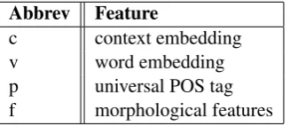
We use limited number of continuous embeddings in parser model. These are POS, word, context, and morphological feature embeddings. Word and context embeddings are pre-trained and not fine-tuned during training. POS and morphological feature embeddings are randomly initialized and learned during training.

Abbrev Feature

c context embedding v word embedding p universal POS tag f morphological features

Table 1: Possible features for each word

3.4 Morphological Feature Embeddings

We introduce morphological feature embeddings, which differs from (Dyer et al., 2015), as an ad-ditional input to our model. Each feature is rep-resented with 128 dimensional continuous vector.

We experiment that vector sizes lower than 128 reduces the performance of a parser, and higher than 128 does not bring further enhancements. We formulate morphological feature embeddings by adding feature vectors of a word. For exam-ple, suppose we are given a wordit with follow-ing morphological features: Case=Nom and Gen-der=Neut and Number=Sing and Person=3 and PronType=Prs. We basically sum corresponding 5 unique vectors to provide morphological feature embedding. However, our experiments suggest that not all languages benefit from morphological feature embeddings. (See section4for details)

3.5 Dependency Label Embeddings

Each distinct dependency label defined inCoNLL

2018 UD Shared Taskrepresented with a 128

di-mensional continuous vector. These vectors com-bined to construct hidden states in tree-RNN part of our model. We randomly initialize these vectors and learned during training.

3.6 ArcHybrid Transition System

We implement the ArcHybrid Transition System which has three components, namely a stack of tree fragmentsσ, a buffer of unused wordsβ and a setAof dependency arcs,c = (σ, β, A). Stack is empty, there is no any arcs and, all the words of a sentence are in buffer initially. This system has 3 type of transitions:

• shift(σ, b|β, A) = (σ|b, β, A)

• leftd(σ|s, b|β, A) = (σ, b|β, A∪ {(b, d, s)})

• right_d(σ|s|t, β, A) = (σ|s, β, A∪ {(s, d, t)})

where|denotes concatenation and(b, d, s)is a de-pendency arc between b (head) and s (modifier) with labeld. The system terminates parsing when the buffer is empty and the stack has only one word assumed to be the root.

3.7 Tree-stack LSTM

e3

e1 e2 e4 e5 e6 e7

c2

Wd

d1 20

(c) Context Encoder

e2

e a r n e

(b) Word Encoder

d2 20

<s> e

e Upos =

verb Mood = indicative

a r n Upos = verb a r n

Mood = indicative

Tense = past

Tense = past

</s>

d

Figure 1: MorphNet illustration for the sentence”Bush earned 340 points in 1969” and target word ”earned”.

. . . Case=Nom|Gender=Neut|Number=Sing|Person=3|PronType=Prs ...

IT It

Figure 2: Morphological feature embeddings ob-tained by adding individual feature embeddings

Our model differs from (Dyer et al.,2015) by rep-resenting actions and dependency relations sep-arately and including morphological feature em-beddings. The transition system (see section 3.6

for details) is also different from theirs.

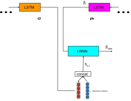
Buffer’sβ-LSTM is initialized with zero hidden state, and fed with input features from last word to the beginning. Similarly, stack’sσ-LSTM is also initialized with zero hidden state and fed with in-put features from the beginning word to the last word of a stack. Actions’ LSTM is also started with zero hidden state, and updated after each ac-tion. Inputs toσ-LSTM andβ-LSTM are updated via tree-RNN.

We update either buffer’s or stack’s input em-beddings based on parsing actions. For instance, suppose we are givenβi a top word in buffer and

σi a final word in stack. The lef td transition

taken in current state. tree-RNN uses concatena-tion of previous embedding, σi, and dependency

relation embedding (explained in3.5) as a hidden

ht−1.Input of a tree-RNN is a previous word

LSTM LSTM LSTM

w_i+2 w_i+1

w_i

Figure 3: β −LST M processing a sentence. It starts to read from right to left. Each vector ((wi)

represents the concatenation of POS, language and morph-feat embeddings.

LSTM LSTM LSTM

s_i s_i+1 s_i+2

Figure 4: σ − LST M processing a sentence. It starts to read from left to right. Each input (si) is transformed version of initial feature

vec-tor. Transformations are based on local transitions see3.6for details.

bedding,βi. Outputht becomes a new word

depicts this flow. Similarly to left transition, right transition updates the stack’s second top word. Hidden state of an RNN is calculated by concate-nating stack’s top word and dependency relation.

There are 73 distinct actions for shift, labeled left and labeled right actions. We randomly ini-tialize 128 dimensional vector for each labeled ac-tion and shift. These vectors become an input for action-LSTM shown in Figure6.

t-RNN LSTM LSTM

β_i

concat ht-1

β_new

Dependency Relation

Figure 5: Buffer word’s embedding update based on left move. Inputs are old embeddings obtained from Table3.3

.

Concatenation of stack’s LSTM, buffer’s LSTM and actions’ LSTM’s final hidden layer becomes an input to MLP which outputs the probabilities for each transition in the next step.

3.8 Training

Our training strategy varies based on training data sizes. We divide datasets into 4 parts: 100k to-kens or more, toto-kens in between 50k and 100k, and more than 20k less than 50k tokens.

For languages having more than 50k tokens in training data, we employ morphological feature-embeddings as an additional input dimension (see Figure2). However, for languages having tokens less than 50k we do not use this feature dimen-sion. Finally we realize that the languages with more than 100k tokens, using morphological fea-ture embeddings does not improve parsing perfor-mance but we use that additional feature dimen-sion.

We use 5-fold cross validation for languages without development data. We do not change the LSTMs’ hidden dimensions, but record the num-ber of epochs took for convergence. The average

of these epochs is used to train a model with whole training set.

3.8.1 Optimization and Hyper-Parameters

We conduct experiments to find best set of hyper-parameters. We start with a dimension of 32 and increase the dimension by powers of two un-til 512 for LSTM hiddens, 1024 for LM matrix (explained in below). We report the best hyper-parameters in this paper. Although the perfor-mance does not decrease after the best setting, we choose the minimum-best size not to sacrifice from training speed.

All the LSTMs and tree-RNN have hidden di-mension of 256. The vectors extracted from LM having dimension of 950, but we reduce that to 512 by a matrix-vector multiplication. This matrix is also learned. We use Adam optimizer with de-fault parameters. (Kingma and Ba,2014).Training is terminated if the performance does not improve for 9 epochs.

4 Results

In this section we inspect our best/worst results and the conclusions we obtain duringCoNLL 2018

UD Shared Taskexperiments.

We submit our system to CoNLL 2018 UD Shared Taskas ”KParse” team. Our scoring is pro-vided under the officialCoNLL 2018 UD Shared Task website.1 as well as in Table 4.1. All ex-periments are done with UD version 2.2 datasets (Nivre et al., 2018) and (Nivre et al., 2017) for training and testing respectively. The model im-proves performance by reducing hand-crafted fea-ture selection. In order to analyze our tree-stack LSTM, we compare that model withKırnap et al.

sharing similar feature interests and transition sys-tem with our model. The difference between these two models is that Kırnap et al. based on hand-crafted feature selection from state, e.g. number of left children of buffer’s first word. However, tree-stack LSTM only needs raw features and previous parsing actions.

Our model comparatively performs better with languages less than 50k training tokens, e.g. sv lines and hu szeged and tr imst. However, when the number of training examples increases the performance improve slightly saturates, e.g. ar padt, en ewt. This may be due to conver-gence problems of our model. This conclusion

1

t-RNN

Head word

Dependent word Dependency Relation

LSTM

LSTM _{LSTM LSTM}

LSTM

LSTM LSTM _A

Concat MLP

Figure 6: End-to-end tree-stack model composed of 4 main components, namely,β-LSTM,σ-LSTM and actions’ LSTMs and the tree-RNN.

Lang code Kırnap et al. New Model

tr imst 56.78 58.75 hu szeged 66.21 68.18 en ewt 74.87 75.77 ar padt 67.83 68.02 cs cac 83.39 83.57 sv lines 71.12 74.81

Table 2: Comparison of two models

is also agrees with our official ranking inCoNLL

2018 UD Shared Taskbecause our ranking in

low-resource languages is 10, but general ranking is 16.

We next analyze the performance gain by in-cluding morphological features with languages training token in between 50k and 100k. As we de-duce from Table3, tree-stack LSTM benefits from morphological information with mid-resource lan-guages. However, we could not gain the similar

Lang code Morp-Feats no Morp-Feats

ko gsd 73.74 72.54 got proiel 54.33 53.24 id gsd 75.76 73.97

Table 3: Morphological feature embeddings in some languages having tokens more than 50k and less than 100k in training data

performance enhancement with languages more than 100k training tokens.

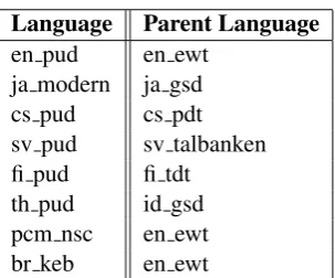
4.1 Languages without Training Data

We list our selections in Table4.

Language Parent Language

en pud en ewt ja modern ja gsd cs pud cs pdt sv pud sv talbanken fi pud fi tdt

th pud id gsd pcm nsc en ewt br keb en ewt

Table 4: Our parent choices in languages without train data

5 Discussion

We use tree-stack LSTM model in transition based dependency parsing framework. Our main motiva-tion for this work is to reduce the human designed features extracted from state components. Our re-sults prove that the model is able to learn better than its predecessors. Moreover, we examine that the model performs better in languages with low resources compared in CoNLL 2018 UD Shared Task. We also constitute morphological feature embeddings which become useful for dependency parsing. All of our work is done in transition based dependency parsing, which sacrifices performance due to locality and non projectiveness. This study opens a question on adapting the tree-stack LSTM in graph based dependency parsing. Our code is publicly available at https://github.com/

kirnap/ku-dependency-parser2.

Acknowlegments

This work was supported by the Scientific and Technological Research Council of Turkey (T ¨UB˙ITAK) grants 114E628 and 215E201.

References

Chris Alberti, Daniel Andor, Ivan Bogatyy, Michael

Collins, Dan Gillick, Lingpeng Kong, Terry

Koo, Ji Ma, Mark Omernick, Slav Petrov,

Chayut Thanapirom, Zora Tung, and David

Weiss. 2017. Syntaxnet models for the conll

2017 shared task. CoRR abs/1703.04929. http://arxiv.org/abs/1703.04929.

Miguel Ballesteros, Chris Dyer, and Noah A Smith. 2015. Improved transition-based parsing by

mod-eling characters instead of words with lstms. arXiv

preprint arXiv:1508.00657.

Danqi Chen and Christopher D Manning. 2014. A fast and accurate dependency parser using neural

net-works. InEMNLP. pages 740–750.

Erenay Dayanık, Ekin Aky¨urek, and Deniz Yuret. 2018. Morphnet: A sequence-to-sequence model that combines morphological analysis and

disam-biguation. arXiv preprint arXiv:1805.07946.

Timothy Dozat, Peng Qi, and Christopher D Manning.

2017. Stanford’s graph-based neural dependency

parser at the conll 2017 shared task. Proceedings

of the CoNLL 2017 Shared Task: Multilingual

Pars-ing from Raw Text to Universal Dependenciespages

20–30.

Chris Dyer, Miguel Ballesteros, Wang Ling, Austin

Matthews, and Noah A. Smith. 2015.

Transition-based dependency parsing with stack long short-term memory. CoRR abs/1505.08075. http://arxiv.org/abs/1505.08075.

Georg Heigold, Guenter Neumann, and Josef van Gen-abith. 2017. An extensive empirical evaluation of character-based morphological tagging for 14

lan-guages. In Proceedings of the 15th Conference of

the European Chapter of the Association for Com-putational Linguistics: Volume 1, Long Papers. vol-ume 1, pages 505–513.

Sepp Hochreiter and J¨urgen Schmidhuber. 1997. Long

short-term memory. Neural Comput. 9(8):1735–

1780.https://doi.org/10.1162/neco.1997.9.8.1735.

Diederik Kingma and Jimmy Ba. 2014. Adam: A

method for stochastic optimization. arXiv preprint

arXiv:1412.6980.

Eliyahu Kiperwasser and Yoav Goldberg. 2016.

Sim-ple and accurate dependency parsing using bidi-rectional LSTM feature representations. CoRR

abs/1603.04351.http://arxiv.org/abs/1603.04351.

¨

Omer Kırnap, Berkay Furkan ¨Onder, and Deniz Yuret.

2017. Parsing with context embeddings.

Proceed-ings of the CoNLL 2017 Shared Task: Multilingual Parsing from Raw Text to Universal Dependencies pages 80–87.

Kimmo Koskenniemi. 1983. Two-level model for

mor-phological analysis. In IJCAI. volume 83, pages

683–685.

Joakim Nivre et al. 2017. Universal Dependencies

2.0 CoNLL 2017 shared task development and test

data. LINDAT/CLARIN digital library at the

Insti-tute of Formal and Applied Linguistics, Charles

Uni-versity, Prague, http://hdl.handle.net/

11234/1-2184. http://hdl.handle.net/11234/1-2184.

Joakim Nivre et al. 2018. Universal

Dependen-cies 2.2. LINDAT/CLARIN digital library at the Institute of Formal and Applied

Lin-guistics, Charles University, Prague, http:

//hdl.handle.net/11234/1-1983xxx.

Language LAS MLAS BLEX Ranks Language LAS MLAS BLEX Ranks

af afribooms 78.12 65.12 63.93 17-15-19 ar padt 68.02 58.05 61.21 16-11-13 bg btb 84.53 75.58 77.63 20-16-9 br keb 8.91 0.35 1.77 19-15-19 bxr bdt 9.93 0.49 0.69 18-22-23 ca ancora 85.89 77.22 77.22 18-17-17 cs cac 83.57 75.3 77.24 19-12-18 cs fictree 82.67 71.93 75.31 18-15-16 cs pdt 81.43 73.77 71.44 21-21-22 cs pud 78.69 64.14 84.52 18-19-17 cu proiel 59.42 46.96 81.55 23-22-21 da ddt 76.4 67.05 63.09 17-15-19 en ewt 75.77 66.78 68.76 20-20-18 en gum 76.44 65.19 64.32 16-12-15 de gsd 71.59 46.87 35.41 17-8-23 el gdt 83.34 65.74 66.6 16-14-18 en lines 73.96 64.91 62.76 17-15-19 en pud 78.41 66.16 69.25 19-19-17 es ancora 84.99 76.71 77.06 18-17-16 et edt 74.52 65.7 63.5 20-19-17 eu bdt 74.55 63.11 61.25 17-13-18 fa seraji 81.18 74.84 71.65 17-16-14 fi ftb 75.84 65.53 67.91 17-16-11 fi pud 81.55 74.18 66.29 13-12-10 fi tdt 78.42 70.4 65.89 16-15-12 fo oft 22.5 0.29 5.44 20-19-20 fr gsd 81.07 72.07 73.96 19-19-17 fr sequoia 84.36 76.56 71.33 14-10-20 fr spoken 57.32 15 57.76 10-10-10 fro srcmf 76.92 67.85 71.35 20-19-20 ga idt 63.13 34.36 40.76 13-19-16 gl ctg 79.02 66.13 71.12 14-14-9 gl treegal 70.45 52.15 56.38 10-9-9 got proiel 54.33 40.58 40.51 24-24-22 grc perseus 55.03 34.19 37.0 20-15-16 grc proiel 62.11 43.92 37.00 22-21-20 he htb 58.28 45.06 48.09 18-16-16 hi hdtb 86.86 70.44 79.98 20-17-15 hr set 81.6 65.23 68.74 17-8-18 hsb ufal 30.81 6.22 15.39 8-9-7 hu szeged 68.18 51.13 50.53 14-20-21 hy armtdp 24.58 7.24 6.96 12-9-21 id gsd 75.51 65.02 63.92 17-13-17 it isdt 85.80 75.5 70.16 22-21-22 it postwita 70.03 56.04 47.53 13-12-20 ja gsd 73.30 59.46 59.89 14-14-20 ja modern 23.35 8.94 10.13 5-4-5 kk ktb 23.86 5.98 8.02 11-11-13 kmr mg 23.39 3.97 7.56 15-15-16 ko gsd 73.74 67.31 60.52 19-18-16 ko kaist 78.81 71.49 65.29 19-19-16 la ittb 75.79 71.49 71.66 20-19-19 la perseus 51.6 33.65 38.04 11-8-8 la proiel 59.35 46.36 51.13 20-19-19 lv lvtb 72.33 57.08 60.54 16-13-14 nl alpino 78.83 64.22 65.79 17-16-15 nl lassysmall 76.70 63.97 64.58 16-15-15 no bokmaal 82.32 37.93 73.52 20-19-18 no nynorsk 80.57 70.78 72.27 20-19-17 no nynorsklia 53.33 41.01 44.46 13-10-11 pcm nsc 15.84 5.3 13.61 10-1-11 pl lfg 86.12 71.96 76.71 21-21-20 pl sz 82.83 63.76 73.05 16-17-14 pt bosque 82.71 68.01 73.07 18-17-15 ro rrt 80.90 72.39 72.59 17-14-14 ru syntagrus 82.89 56.8 75.48 20-19-18 ru taiga 60.55 39.41 44.05 11-9-9 sk snk 75.75 53.49 61.0 20-20-16 sl ssj 78.18 62.94 69.49 16-18-14 sl sst 48.77 34.66 39.82 10-11-9 sme giella 53.39 39.13 41.75 19-19-15 sr set 80.85 67.46 72.09 20-19-16 sv lines 74.81 59.72 67.35 17-15-15 sv pud 70.77 43.04 54.67 16-12-15 sv talbanken 77.91 69.25 69.87 17-16-17 th pud 0.74 0.04 0.44 7-8-8 tr imst 58.75 48.28 49.84 15-12-13 ug udt 57.04 36.63 44.44 16-16-14 uk iu 76.5 36.63 65.5 16-16-13 ur udtb 78.12 51.25 64.66 17-15-15 vi vtb 40.48 33.88 36.03 16-14-15 zh gsd 59.76 50.87 53.11 19-15-18

Milan Straka, Jan Hajiˇc, and Jana Strakov´a. 2016. UD-Pipe: trainable pipeline for processing CoNLL-U files performing tokenization, morphological

anal-ysis, POS tagging and parsing. In Proceedings

of the 10th International Conference on Language

Resources and Evaluation (LREC 2016). European