II. OPEN LOOP RESPONSE

Abstract_{— This study is based upon evaluating the}

performance and power consumption of a least effort controller for a turbo-jet engine. The paper emphasizes that the least effort control technique gives comparable transient performance and disturbance recovery characteristics with referenced results, obtained from Nyquist array and optimal control methods. It also provides a simpler controller than those given by these techniques whilst dissipating minimum control energy leading to minimum heat, wear and maintenance costs. Rapid implementation of this design theory for aircraft engines and for general multivariable applications is advocated.

Index Term— multivariable, control, least-effort, INA, optimal

I. INTRODUCTION

he fuel flow rate and the nozzle area changes are the manipulated input variables, while high and low pressure spool speeds, are the output variables, for the turbo-jet engine considered in this contribution. Multivariable system analysis presents further restrictions on the classical control problem, such as output interaction regulation, integrity confirmation and stability assessment. The pilot control of aircraft jet engines, especially during the critical flight modes, such as at takeoff and landing are investigated. The reliability and rapid response of the engine’s control system is essential, for the safe approach and deck landing of aircraft. Random disturbances on the control systems, of aircraft engines, are to be expected due to air turbulence and during varying operational flight modes. This would affect the performance of the aircraft and the control system which should be designed to limit the effect of output changes and random disturbances.

Aircraft have limited power supplies. Consequently, research and development aimed at minimizing the fuel consumption of aircraft engines, from a mechanical point of view are important. However, the problem of the energy consumption of the gas turbine control system itself, to minimize wear, maintenance, noise and heat generation whilst reducing the deterioration of the control system components has been neglected.

This paper exploits recent advances in multivariable system control emphasizing the minimization of the control effort required for the regulation of the engine model [1]. The methodology applied is to design a Least Effort Controller [2] for a twin-spool turbo-jet engine model. The proposed controller also addresses problems such as closed

Manuscript received June 18, 2012; revised July 28, 2012. This work was supported in part by the British University in Dubai, research grant 68250.

Professor R. Whalley, Author is the Head of Systems Engineering Programme at the British University in Dubai, P.O. Box 345015, Dubai-UAE, phone: +971-43644666; fax: +971-43664698; e-mail: robert.whalley@ buid.ac.ae).

Mr. T. El-Hassan, is PG research student at the British University in Dubai, P.O. Box 345015, Dubai-UAE: e-mail: [email protected].

loop stability improving thereby the transient and aircraft steady state responses whilst enhancing the disturbance rejection properties of the system.

The case study considered herein is in respect of a twin spool turbo-jet engine, and the proposed controller will be compared with previous designs [3] and [4]. Substantial simplification of the controller is achieved whilst maintaining the closed loop design characteristics specified for existing designs.

II.OPENLOOPRESPONSE

The general transfer function for the jet engine, model as shown in [1], is given by:

∆()

∆() = .

.(.)_..

.

(.)

_..

0

0

∆,

∆ !, (1)

An investigation of the open loop responses requires the simulation of the system model following a unit step change on each input. These are as shown in Fig 1 and Fig. 2. From Fig. 1, the simulation exhibits over damped behaviour for both outputs and a settling time of almost 3 seconds with an output interaction of almost 570%. The second output is for the low-pressure spool speed, ∆(). Fig. 2 again shows this to be over damped responses for both outputs and a settling time of approximately 4 seconds, with approximately 75% interaction is evident.

Disregarding the substantial output coupling, the system model is stable and dynamically well behaved. Therefore, the control strategy herein will be focused on reducing the system output interaction whilst improving the transient response. The control system should be such that changes in any system input will not cause a significant change in the remaining outputs. A ten percent limit on the steady state interaction between outputs, for any input changes, is normally acceptable.

The closed loop response should also be stable, and well behaved with overshoots of less than 20%. An improvement in the system response is required and the settling time must be reduced.

Since the system model represents a jet engine, random disturbances are to be expected. Air turbulence and changes in the aircraft flight mode (e.g. takeoff, cruise) result in natural air turbulence disturbances. The robustness of the control system and any change in the model parameters should also be considered. An investigation of the disturbance recovery response is also required. Importantly, this paper investigates the energy consumed by the closed loop control action.

Turbo-Jet Engine Multivariable Control

R. Whalley and T. El-Hassan

III. LEASTEFFORTCONTROLMETHODOLOGY In the design procedure outlined here, a dual loop approach is adopted, where an inner loop will be utilized to secure acceptable dynamics and an outer loop and the pre-compensator will primarily be employed to satisfy disturbance-output conditions, as shown in [5].

The transformed open loop system equation is:

#() = $()%() & '() (2) and if the control law for the proposed feedback is

%() = (())*̅() , -()#(). & /(*() , 0#()) (3)

where in (2) and (3) there are m independent inputs, disturbances, and outputs and

( ), 0 1, 1 .

F=Diag f <f< ≤ ≤j m Since the inner loop controller is:

(())*̅() , -()#().

this will be used to satisfy the specified dynamic behavior of the closed loop system while the outer loop controller, given by:

/(*() , 0#())

will be utilized to secure the required steady state interaction and disturbance recovery capacity of the system. With *2() = 0, the closed-loop equation becomes:

#() = (34& $()((() 56 -() & /0))7₈

($() /*() & '()) (4) If a steady-state matrix S: is now selected such that

#(0) = ;*(0)

then from (4), with = 0 :

/ = ($(0)7_{& ((0) 56 -(0));}

(3 , 0;)7 (5) At low frequencies,

$()/ ≅_{1 , > (3}1 4& $()((0) 56 -(0))

Consequently, (6) on approaching steady-state conditions becomes:

#() = 34*() & ;()'() (7) where the low frequency sensitivity matrix is:

;() = (1 , >)(34& $()(() 56 -())7, 0 6 > 6 1

Evidently, from (7), if Ss=Im steady-state non-interaction

would be achieved. Moreover, as f is increased,> 6 1, there will be increasing steady-state disturbance rejection , with imposition of the stability constraint.

For implementation purposes, a conventional multivariable regulator structure comprising a forward path

@() and feedback path compensator A() could be easily be computed from (4).The input-output relationship would be:

#() = (34& $()@()A())7_{)$@()*() & '(). (8)}

On comparing (4) and (8), evidently

@() = / (9) and @()A() = (() 56 -() & /0

A() = /7_{(() 56 -() & 0 (10)}

enabling the employment of established feedback structures.

A. _{Inner Loop Analysis}

The open loop system $() is assumed to be an m 8

m linear, regular, proper, or strictly proper realization which admits a general factorization of:

$() = B()C()₍₎D()E() (11) where B(), (), D(), E(), and the elements of F(:)

G(:)∈ HJ, s ∈ L

In (11), B() contains the left (row) factors of $() , while D() contains the right (column) factors, and E() contains the transformed finite time delays, such that the

M 8 M matrices comprising (11) are:

(

)

(

)

(

)

( ) ( ) / ( ) , ( ) ( ) / ( )

and ( ) j 1 ,

j j j j

sT

L s Diag s p s R s Diag s q s

s Diag e i j m

λ ρ

−

= =

Γ = ≤ ≤

and det ( )A s ≠0,with elements:

NOP() = NOP47_{& QOP}47_{& ⋯ & SOP 1 T U, V T M (12)}

As the input-output-disturbance relationship is:

#() = $()%() & '() (13)

and if the inner-loop controller is:

%() = (())*̅() , -()#(). (14)

Then, combining (13) and (14) yields:

#() = (34& $()(() 56 -())7_{($()(()*̅() &}

'() (15) Any finite time delays in E() could be ordered with

WO X WP , 1 T V T M , U Y V , so that the forward path gain vector can be arranged as:

(() = )(()Z7[\]7\^__{, (()Z}7[\]7\^_

, … . , ((), … . . , (4()Z7(\]7\^)_.\ ₍₁₆₎

Since:

(P() = (P∅P() and -P() = -PbP() 1 T V T M where

∅P() and bP() are proper or strictly proper , stable , realizable , minimum phase functions , then they could be selected such that (15) becomes:

#() = c34& Z7\]d()B()C()

()(() 56 -()e

7 8 cd()B()C()₍₎(Z7\]*() & '()e ₍₁₈₎

where:

( = ((, (, … . , (4)\ ₍₁₉₎

and

- = (-, -, … . , -4) (20) f() = g_{& N}g7_{& ⋯ & N}

and fZh cd()NO,P()e 6 ( 1 T U, V T M The determinant required in (18) is:

fZi j34& Z7\]d()B()C()

()(() 56 -()k = 1 &

Z7\]d() 6 -C()

()( 5 (21)

The inner product in (21), may be expressed as:

6 -()( 5=

)1, , … . , 47_{. l}

S S ⋯ S44

⋮ Q N

⋮

Q

N …⋱…

⋮ Q44 N44 o l (- (-⋮ (4-4

o (22)

If in equation (22), the gain ratios are:

(= d(, (= d(, … . (4= d47( (23)

and

6 -()( 5= Q() (24)

then (24) implies that:

() .- = (Q47, Q47, … . , Q)\ (25)

where:

Q

= l

S& Sd& S4d47 ⋮ S& Sd& S4d47

⋮ ⋮

Q& Qd& Q4d47

N& Nd& N4d47 ⋮ Q⋮ N& Qd& Nd& Q4d47& N4d47

⋮ ⋯S4& S4d& S44d47

⋮

⋮ ⋯Q4& Q4d& Q44d47

⋮ ⋯N4& N4d& N44d47qr r r r s

B. _Optimization

To detect the absolute minimum control effort required, under closed-loop conditions with arbitrary disturbances entering the system, a performance index representing the energy dissipated should be defined. The control effort, at time t is proportional to:

(|(-| & |(-| & ⋯ |(4-|)|#(i)|

& (|(-| & |(-| & ⋯ |(4-|)|#(i)| & ⋯

& (|(-4| & |(-4| & ⋯ |(4-4|)|#4(i)|

Hence, the control energy costs, under these conditions, are proportional to:

v(i) = w [∑ (4

Oy ∑ -4Py P#P(i)_fi zy\{

zy (26)

Then for arbitrary changes in the transformed output vector #(i), following arbitrary disturbance changes:

| = ∑ (4Oy ∑ -P4Py (27)

If the relationships:

(= d( , (= d(… . . (4= d47(

are adopted then (27) can be written as:

(

) (

)

1 2 1

1 T T

m

J= +n +n +n− b Q− Q b−

C. _{Disturbance Rejection Analysis}

The employment of the minimum control effort would not, in general, achieve required disturbance recovery conditions. To provide this, the outer-loop feedback gain f

should be increased 0 6 > 61.0, as indicated by (7). For further analysis details, see [5].

D. _{Stability of Combined System}

The stability condition is dependent on the denominator of the input-output relationship for the complete, closed-loop system which is given by (8). Consequently, the outer – loop feedback gain matrix F is given by

( ) 0 1

F=Diag f <f<

Then the denominator of equation (8) may be computed from:

fZi ~34+ $ ( >< ℎ_{1 − >} +$0 7_>

1 − > €

From this expression, it is clear that the elements of the feedback-compensator matrix become infinite as > → 1. This would always result in closed-loop system instability. Consequently, 0 < f <1, is mandatory.

IV. LEASTEFFORTCONTROLLER

In the design procedure outlined here, the inner loop will be utilized to secure acceptable dynamics, the outer loop and the pre-compensator will be employed to satisfy disturbance-rejection conditions. For the gas turbine model, according to (1) is:

$ = l 1.496

+ 2 951.5 + 1.898_{+ 3.225 + 2.525}

8.52

+ 2 1240 + 2.037_{+ 3.225 + 2.525}

o l 10

+ 10 0 0 _{+ 100}100 o $ = . .. _.. . . _.. 0

0 

0

0 1€ 

0

0 1€

Multiplying the first three matrices and rearranging in the

form : $ = BCDE

$ = .[.._ . .[.._ .€ _..  0

0 1€

where B = 3 , E = 3, D = 

0

0 1€, =

14.96_{85.2+ 3.225 + 2.525 124000 + 2.037 + 2} + 3.225 + 2.525 95150 + 1.898 + 2

( 100) ( 10) 0 . 0 1

s s

 _{+ +} 

 

 

The approximation:

h= 14.96

_{+ 3.225 + 2.525}

_{+ 3.225 + 2.525 + 2 + 100}

≈ _{+ 100}15.418 + 18.887_{+ 3.225 + 2.525}

h= 85.2

_{+ 3.225 + 2.525}

_{+ 3.225 + 2.525 + 2 + 100}

≈ _{+ 100}87.8082 + 107.565_{+ 3.225 + 2.525}

h=_{+ 3.225 + 2.525 + 2 + 100}95150 + 1.898 + 2

= _{+ 100}95150 + 1.898_{+ 3.225 + 2.525}

h=_{+ 3.225 + 2.525 + 2 + 100}124000 + 2.037 + 2

=_{+ 3.225 + 2.525 + 100}124000 + 2.037

will be employed.

h =_f

≈j 15.418 + 18.887

95150 + 180594.7 87.8082 + 107.565 124000 + 252588k

_{+ 3.225 + 2.525 + 100}

Then according to (22):

( ) ( )

( ) ( )

1 1 2 1

1 2 2 2

15.418 18.887 95150 180594.7

87.8082 107.565 124000 2 ( )

52 85 8

s k h s k h

s k h s

hA k

k h

s + + +

+ +

=

+ +

< >

= [1 ] j18.887 180594.7 107.565 252588_{15.418 95150 87.8082 124000k l} (ℎ

(ℎ

(ℎ

(ℎ

o

According to (23), the gain ratio n is substituted to formulate the Q matrix

with

k

=

1 yielding:

= j18.887 + 180594.7d 107.565 + 252588d_{15.418 + 95150d 87.8082 + 124000dk}

From (24), < ℎC( >=Ž

where: f = + 3.225 + 2.525 + 100 =

+ 1.34 + 1.8866 + 100

If Q = s + 1.5 , so that this zero will attract the pole at ( = −1.34) reducing the settling time, and assuring closed loop stability.

Substituting for Q and yields the performance index:

| =

_.7.

.

7.. (31)

Fig. 4, shows the performance index | against gain ratio d. To find the absolute minimum value of the performance index, differentiating the J function with respect to gain ratio and equating to zero so that:

‘| ‘d = 0

reveals that there are four supremum values for J where min

J

d = −458.58735 “ℎZ*Z | = 0.218Z − 18 (minimum) as shown in Fig. 4.

Hence, the inner loop forward gain values becomes with

1 1:

k =

1 (0)

458.58735

k = 

−

 

(32) Now, substituting , Q = j 1

1.5k into (25), yields the inner

loop feedback gain values which are

h0 =•_g–—˜

— = [−0.8854e − 7, 0.5035e − 7] (33)

To design the outer loop, the feed forward and feedback gain matrices k(0), h(0), Ss, G(0) and F are required.

since

$ =< ℎ_{f ( > D}

then

( = (. D = j_{−458.58735k }1 0

0 1€ (34) (0 = j_−458.5874k10 and ℎ0 = [−0.8854Z −

7 0.5035Z − 7] (36) The steady state open loop transfer function matrix is given by G(0)and the steady state interaction due to output coupling would be restricted in closed loop to 10% if:

;= j 1 0.1_{0.1 1 k} (38) Investigation of the effect of increasing feedback gains from 0.1 to 0.9 on closed loop response and disturbance suppression will be studied in order to complete the control system strategy.

For 0 = j0.9 0

0 0.9k (45) / = j−8.588 −5.053_{0.0904 0.0797k} (46)

A =

.: :

.: : .:

:

.: :

=

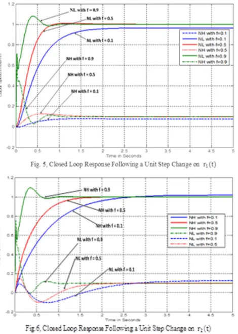
j 0.899_0.00162 0.000542_{0.8991 k} (47) For values of f <0.9 the compensator P and H have elements of smaller moduli. For comparison purposes, the closed loop response was simulated using the three designs of outer loop feedback gain f. Following a unit step change on the reference inputs of jet nozzle cross sectional area

Also, the effect of increasing outer loop feedback gain f

from 0.1 to 0.9, on the system disturbance rejection transient following a unit step change on disturbance δt and then

δt, respectively will be compared for the three system designs using >= 0.1, >= 0.5 Ndf >= 0.9 as shown in Fig. 7 and Fig. 8.

V.CONTROLENERGYDISSIPATION

The controller for the inverse Nyquist and optimal designs are presented in Fig. 9. The energy consumed by each of the three controllers can be computed form:

(

)

600

2 2

1 2

0

( ) ( ) ( )

t

E s u t u t dt

=

=

∫

VI. CONCLUSIONS

The least effort controller’s responses are stable, rapid and well behaved. Despite the strong coupling exhibited by the twin-spool jet engine, this controller succeeds in reducing the output interaction, as specified. This reflects the flexibility of its design philosophy, giving freedom to enhance the performance and the closed loop response of multivariable systems. The inner loop design provides an effective method for improving the transient response. Meanwhile, the outer loop design is used to reduce output interaction enhancing the disturbance recovery performance, thereby. The entire strategy is based upon minimizing the control effort required which is a commendable specification requirement.

The least effort controller gives comparable performance characteristics with any of the published results. It also requires less control effort than these methods which employ perfect integrators or alternatively, relatively high gains.

ACKNOWLEDGMENT

The Professor Whalley wishes to acknowledge the support and encouragement for this research provided by the Vice Chancellor, The British University in Dubai-UAE.

REFERENCES

[1] CHUGHTAI S. S AND MUNRO, N., “DIAGONAL

DOMINANCE USING LMI”, IEE PROC., CONTROL

THEORY AND APPLICATIONS,VOL.151,NO.2,2004, PP. 225-23.

[2] Whalley, R. and Ebrahimi, M, “Automotive Gas Turbine Regulation”, IEEE Trans. Contr. Syst. Technol., (2004), pp.465-473.

[3] Mueller, G, “Linear Model of 2-Shaft Turbojet and Its Properties”, Proc. IEE, Vol.118, No. 6, 1971, pp. 813-815.

[4] McMorran, P. D, “Design of Gas-Turbine Controller Using Inversed Nyquist Method”. Proc. IEE, Vol. 117, 1970, pp. 2050-2056.