Multichannel Variable-Size Convolution for Sentence Classification
Wenpeng YinandHinrich Sch¨utze Center for Information and Language Processing
University of Munich, Germany [email protected]
Abstract
We proposeMVCNN, a convolution neu-ral network (CNN) architecture for sen-tence classification. It (i) combines di-verse versions of pretrained word embed-dings and (ii) extracts features of multi-granular phrases with variable-size convo-lution filters. We also show that pretrain-ing MVCNN is critical for good perfor-mance. MVCNN achieves state-of-the-art performance on four tasks: on small-scale binary, small-scale multi-class and large-scale Twitter sentiment prediction and on subjectivity classification.
1 Introduction
Different sentence classification tasks are crucial for many Natural Language Processing (NLP) ap-plications. Natural language sentences have com-plicated structures, both sequential and hierarchi-cal, that are essential for understanding them. In addition, how to decode and compose the features of component units, including single words and variable-size phrases, is central to the sentence classification problem.
In recent years, deep learning models have achieved remarkable results in computer vision (Krizhevsky et al., 2012), speech recognition (Graves et al., 2013) and NLP (Collobert and We-ston, 2008). A problem largely specific to NLP is how to detect features of linguistic units, how to conduct composition over variable-size sequences and how to use them for NLP tasks (Collobert et al., 2011; Kalchbrenner et al., 2014; Kim, 2014). Socher et al. (2011a) proposed recursive neural networks to form phrases based on parsing trees. This approach depends on the availability of a well performing parser; for many languages and do-mains, especially noisy dodo-mains, reliable parsing is difficult. Hence, convolution neural networks
(CNN) are getting increasing attention, for they are able to model long-range dependencies in sen-tences via hierarchical structures (Dos Santos and Gatti, 2014; Kim, 2014; Denil et al., 2014). Cur-rent CNN systems usually implement a convolu-tion layer with fixed-size filters (i.e., feature detec-tors), in which the concrete filter size is a hyper-parameter. They essentially split a sentence into multiple sub-sentences by a sliding window, then determine the sentence label by using the domi-nant label across all sub-sentences. The underly-ing assumption is that the sub-sentence with that granularity is potentially good enough to represent the whole sentence. However, it is hard to find the granularity of a “good sub-sentence” that works well across sentences. This motivates us to imple-mentvariable-size filtersin a convolution layer in order to extract features ofmultigranular phrases. Breakthroughs of deep learning in NLP are also based on learning distributed word representations – also called “word embeddings” – by neural lan-guage models (Bengio et al., 2003; Mnih and Hin-ton, 2009; Mikolov et al., 2010; Mikolov, 2012; Mikolov et al., 2013a). Word embeddings are de-rived by projecting words from a sparse, 1-of-V encoding (V: vocabulary size) onto a lower di-mensional and dense vector space via hidden lay-ers and can be interpreted as feature extractors that encode semantic and syntactic features of words.
Many papers study the comparative perfor-mance of different versions of word embed-dings, usually learned by different neural net-work (NN) architectures. For example, Chen et al. (2013) compared HLBL (Mnih and Hinton, 2009), SENNA (Collobert and Weston, 2008), Turian (Turian et al., 2010) and Huang (Huang et al., 2012), showing great variance in quality and characteristics of the semantics captured by the tested embedding versions. Hill et al. (2014) showed that embeddings learned by neural ma-chine translation models outperform three
sentative monolingual embedding versions: skip-gram (Mikolov et al., 2013b), GloVe (Pennington et al., 2014) and C&W (Collobert et al., 2011) in some cases. These prior studies motivate us to ex-plore combining multiple versions of word embed-dings, treating each of them as a distinct descrip-tion of words. Our expectadescrip-tion is that the com-bination of these embedding versions, trained by different NNs on different corpora, should contain more information than each version individually. We want to leverage this diversity of different em-bedding versions to extract higher quality sentence features and thereby improve sentence classifica-tion performance.
The letters “M” and “V” in the name “MVCNN” of our architecture denote the multi-channel and variable-size convolution filters, re-spectively. “Multichannel” employs language from computer vision where a color image has red, green and blue channels. Here, a channel is a de-scription by an embedding version.
For many sentence classification tasks, only rel-atively small training sets are available. MVCNN has a large number of parameters, so that overfit-ting is a danger when they are trained on small training sets. We address this problem by pre-training MVCNN on unlabeled data. These pre-trained weights can then be fine-tuned for the spe-cific classification task.
In sum, we attribute the success of MVCNN to: (i) designing variable-size convolution filters to extract variable-range features of sentences and (ii) exploring the combination of multiple pub-lic embedding versions to initialize words in stences. We also employ two “tricks” to further en-hance system performance: mutual learning and pretraining.
In remaining parts, Section 2 presents related work. Section 3 gives details of our classification model. Section 4 introduces two tricks that en-hance system performance: mutual-learning and pretraining. Section 5 reports experimental re-sults. Section 6 concludes this work.
2 Related Work
Much prior work has exploited deep neural net-works to model sentences.
Blacoe and Lapata (2012) represented a sen-tence by element-wise addition, multiplication, or recursive autoencoder over embeddings of com-ponent single words. Yin and Sch¨utze (2014)
ex-tended this approach by composing on words and phrases instead of only single words.
Collobert and Weston (2008) and Yu et al. (2014) used one layer of convolution over phrases detected by a sliding window on a target sentence, then used max- or average-pooling to form a sen-tence representation.
Kalchbrenner et al. (2014) stacked multiple lay-ers ofone-dimensionalconvolution by dynamic k-max pooling to model sentences. We also adopt dynamic k-max pooling while our convolution layer has variable-size filters.
Kim (2014) also studied multichannel repre-sentation and variable-size filters. Differently, their multichannel relies on a single version of pretrained embeddings (i.e., pretrained Word2Vec embeddings) with two copies: one is kept stable and the other one is fine-tuned by backpropaga-tion. We develop this insight by incorporating di-verse embedding versions. Additionally, their idea of variable-size filters is further developed.
Le and Mikolov (2014) initialized the represen-tation of a sentence as a parameter vector, treat-ing it as a global feature and combintreat-ing this vec-tor with the representations of context words to do word prediction. Finally, this fine-tuned vec-tor is used as representation of this sentence. Ap-parently, this method can only produce generic sentence representations which encode no task-specific features.
al., 2014). In our work, there is no limit to the type of embedding versions we can use and they leverage not only the diversity of corpora, but also the different principles of learning algorithms.
3 Model Description
We now describe the architecture of our model
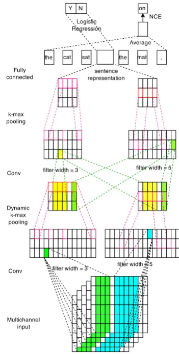
MVCNN, illustrated in Figure 1.
Multichannel Input. The input of MVCNN in-cludesmultichannel feature mapsof a considered sentence, each is a matrix initialized by a differ-ent embedding version. Letsbe sentence length, d dimension of word embeddings and c the to-tal number of different embedding versions (i.e., channels). Hence, the whole initialized input is a three-dimensional array of sizec×d×s. Figure 1 depicts a sentence withs= 12words. Each word is initialized by c = 5 embeddings, each com-ing from a different channel. In implementation, sentences in a mini-batch will be padded to the same length, and unknown words for correspond-ing channel are randomly initialized or can acquire good initialization from themutual-learningphase described in next section.
Multichannel initialization brings two advan-tages: 1) a frequent word can have c representa-tions in the beginning (instead of only one), which means it has more available information to lever-age; 2) a rare word missed in some embedding versions can be “made up” by others (we call it “partially known word”). Therefore, this kind of initialization is able to make use of information about partially known words, without having to employ full random initialization or removal of unknown words. The vocabulary of the binary sentiment prediction task described in experimen-tal part contains 5232 words unknown in HLBL embeddings, 4273 in Huang embeddings, 3299 in GloVe embeddings, 4136 in SENNA embeddings and 2257 in Word2Vec embeddings. But only 1824 words find no embedding from any chan-nel! Hence, multichannel initialization can con-siderably reduce the number of unknown words.
Convolution Layer (Conv). For convenience, we first introduce how this work uses a convo-lution layer on one input feature map to gener-ate one higher-level feature map. Given a sen-tence of length s: w1, w2, . . . , ws; wi ∈ Rd
de-notes the embedding of word wi; a convolution
layer uses sliding filters to extract local features of that sentence. The filter width l is a
param-Figure 1: MVCNN: supervised classification and pretraining.
eter. We first concatenate the initialized embed-dings oflconsecutive words (wi−l+1, . . . ,wi) as
ci ∈ Rld (1 ≤ i < s+l), then generate the
fea-ture value of this phrase aspi (the whole vector p ∈ Rs+l−1 contains all the local features) using a tanh activation function and a linear projection vectorv∈Rldas:
pi = tanh(vTci+b) (1)
[image:3.595.328.504.61.409.2]we keep the property of multi-kernel while extend-ing it to variable-size in the same layer.
As in CNN for object recognition, to increase thenumberof kernels of a certain layer, multiple feature maps may be computed in parallel at the same layer. Further, to increase the size diversity
of kernels in the same layer, more feature maps containing various-range dependency features can be learned. We denote a feature map of the ith layer byFi, and assume totallynfeature maps
ex-ist in layer i−1: F1
i−1, . . . ,Fni−1. Considering a specific filter sizel in layeri, each feature map Fji,lis computed by convolving a distinct set of fil-ters of sizel, arranged in a matrixVi,lj,k, with each feature mapFk
i−1and summing the results:
Fji,l=
n
X
k=1
Vi,lj,k∗Fki−1 (2)
where ∗ indicates the convolution operation and j is the index of a feature map in layer i. The weights inVform a rank 4 tensor.
Note that we usewide convolutionin this work: it means word representations wg for g ≤ 0 or
g≥s+1are actually zero embeddings. Wide con-volution enables that each word can be detected by all filter weights inV.
In Figure 1, the first convolution layer deals with an input withn= 5feature maps.1 Its filters
have sizes 3 and 5 respectively (i.e.,l= 3,5), and each filter hasj = 3kernels. This means this con-volution layer can detect three kinds of features of phrases with length 3 and 5, respectively.
DCNN in (Kalchbrenner et al., 2014) used one-dimensional convolution: each higher-order fea-ture is produced from values of a single dimen-sion in the lower-layer feature map. Even though that work proposed folding operation to model the dependencies between adjacent dimensions, this type of dependency modeling is still lim-ited. Differently, convolution in present work is able to model dependency across dimensions as well as adjacent words, which obviates the need for a folding step. This change also means our model has substantially fewer parameters than the DCNN since the output of each convolution layer is smaller by a factor ofd.
1A reviewer expresses surprise at such a small number of
maps. However, we will use four variable sizes (see below), so that the overall number of maps is 20. We use a small number of maps partly because training times for a network are on the order of days, so limiting the number of parameters is important.
Dynamic k-max Pooling. Kalchbrenner et al. (2014) pool thek most active features compared with simple max (1-max) pooling (Collobert and Weston, 2008). This property enables it to con-nect multiple convolution layers to form a deep architecture to extract high-level abstract features. In this work, we directly use it to extract features for variable-size feature maps. For a given feature map in layeri, dynamic k-max pooling extractski
top values from each dimension andktoptop
val-ues in the top layer. We set
ki= max(ktop,dLL−ise) (3)
wherei∈ {1,2, . . . L}is the order of convolution layer from bottom to top in Figure 1;Lis the total numbers of convolution layers;ktop is a constant
determined empirically, we set it to 4 as (Kalch-brenner et al., 2014).
As a result, the second convolution layer in Fig-ure 1 has an input with two same-size featFig-ure maps, one results from filter size 3, one from filter size 5. The values in the two feature maps are for phrases with different granularity. The motivation of this convolution layer lies in that a feature re-flected by a short phrase may be not trustworthy while the longer phrase containing the short one is trustworthy, or the long phrase has no trustworthy feature while its component short phrase is more reliable. This and even higher-order convolution layers therefore canmake a trade-off between the features of different granularity.
Hidden Layer. On the top of the final k-max pooling, we stack a fully connected layer to learn sentence representation with given dimen-sion (e.g.,d).
Logistic Regression Layer. Finally, sentence representation is forwarded into logistic regression layer for classification.
further exploration of multichannel and variable-size feature detectors.
4 Model Enhancements
This part introduces two training tricks that en-hance the performance of MVCNN in practice.
Mutual-Learning of Embedding Versions. One observation in using multiple embedding ver-sions is that they have different vocabulary cover-age. An unknown word in an embedding version may be a known word in another version. Thus, there exists a proportion of words that can only be partially initialized by certain versions of word embeddings, which means these words lack the description from other versions.
To alleviate this problem, we design a mutual-learning regime to predict representations of un-known words for each embedding version by learning projections between versions. As a result, all embedding versions have the same vocabulary. This processing ensures that more words in each embedding version receive a good representation, and is expected to give most words occurring in a classification dataset more comprehensive ization (as opposed to just being randomly initial-ized).
Let cbe the number of embedding versions in consideration, V1, V2, . . . , Vi, . . . , Vc their
vocab-ularies, V∗ = ∪c
i=1Vi their union, and Vi− =
V∗\Vi (i= 1, . . . , c) the vocabulary of unknown
words for embedding version i. Our goal is to learn embeddings for the words inVi−by knowl-edge from the otherc−1embedding versions.
We use the overlapping vocabulary betweenVi
andVj, denoted asVij, as training set, formalizing
a projection fij from space Vi to space Vj (i 6=
j;i, j∈ {1,2, . . . , c}) as follows:
ˆ
wj =Mijwi (4)
where Mij ∈ Rd×d, wi ∈ Rd denotes the
rep-resentation of word w in space Vi and wˆj is the
projected (or learned) representation of wordwin spaceVj. Squared error betweenwjandwˆj is the
training loss to minimize. We use wˆj = fij(wi)
to reformat Equation 4. Totallyc(c−1)/2 projec-tionsfij are trained, each on the vocabulary
inter-sectionVij.
Let w be a word that is unknown in Vi, but is
known inV1, V2, . . . , Vk. To compute an
embed-ding forwinVi, we first compute thekprojections
f1i(w1), f2i(w2), . . ., fki(wk) from the source
spacesV1, V2, . . . , Vkto the target spaceVi. Then,
the element-wise average off1i(w1),f2i(w2),. . ., fki(wk)is treated as the representation ofwinVi.
Our motivation is that – assuming there is a true representation ofwinVi (e.g., the one we would
have obtained by training embeddings on a much larger corpus) and assuming the projections were learned well – we would expect all the projected vectors to be close to the true representation. Also, each source space contributes potentially comple-mentary information. Hence averaging them is a balance of knowledge from all source spaces.
As discussed in Section 3, we found that for the binary sentiment classification dataset, many words were unknown in at least one embedding version. But of these words, a total of 5022 words did have coverage in another embedding version and so will benefit from mutual-learning. In the experiments, we will show that this is a very ef-fective method to learn representations for un-known words that increases system performance if learned representations are used for initialization.
Pretraining. Sentence classification systems are usually implemented as supervised training regimes where training loss is between true la-bel distribution and predicted lala-bel distribution. In this work, we use pretraining on the unlabeled data of each task and show that it can increase the per-formance of classification systems.
Figure 1 shows our pretraining setup. The “sentence representation” – the output of “Fully connected” hidden layer – is used to predict the component words (“on” in the figure) in the sen-tence (instead of predicting the sensen-tence label Y/N as in supervised learning). Concretely, the sen-tence representation is averaged with representa-tions of some surrounding words (“the”, “cat”, “sat”, “the”, “mat”, “,” in the figure) to predict the middle word (“on”).
Given sentence representations ∈ Rd and
ini-tialized representations of2tcontext words (tleft words andtright words): wi−t,. . .,wi−1,wi+1, . . ., wi+t;wi ∈ Rd, we average the total2t+ 1
vectors element-wise, depicted as “Average” op-eration in Figure 1. Then, this resulting vector is treated as a predicted representation of the mid-dle word and is used to find the true midmid-dle word by means of noise-contrastive estimation (NCE) (Mnih and Teh, 2012). For each true example, 10 noise words are sampled.
where each word needs initialization. (i) Each word in the sentence is initialized in the “Multi-channel input” layer to the whole network. (ii) Each context word is initialized as input to the av-erage layer (“Avav-erage” in the figure). (iii) Each tar-get word is initialized as the output of the “NCE” layer (“on” in the figure). In this work, we use multichannel initialization for case (i) and random initialization for cases (ii) and (iii). Only fine-tuned multichannel representations (case (i)) are kept for subsequent supervised training.
The rationale for this pretraining is similar to auto-encoder: for an object composed of smaller-granular elements, the representations of the whole object and its components can learn each other. The CNN architecture learns sentence features layer by layer, then those features are jus-tified by all constituent words.
During pretraining, all the model parameters, including mutichannel input, convolution parame-ters and fully connected layer, will be updated un-til they are mature to extract the sentence features. Subsequently, the same sets of parameters will be fine-tuned for supervised classification tasks.
In sum, this pretraining is designed to produce good initial values for both model parameters and word embeddings. It is especially helpful for pre-training the embeddings of unknown words.
5 Experiments
We test the network on four classification tasks. We begin by specifying aspects of the implemen-tation and the training of the network. We then report the results of the experiments.
5.1 Hyperparameters and Training
In each of the experiments, the top of the net-work is a logistic regression that predicts the probability distribution over classes given the in-put sentence. The network is trained to mini-mize cross-entropy of predicted and true distri-butions; the objective includes an L2 regulariza-tion term over the parameters. The set of param-eters comprises the word embeddings, all filter weights and the weights in fully connected layers. A dropout operation (Hinton et al., 2012) is put be-fore the logistic regression layer. The network is trained by back-propagation in mini-batches and the gradient-based optimization is performed us-ing the AdaGrad update rule (Duchi et al., 2011)
In all data sets, the initial learning rate is 0.01,
dropout probability is 0.8,L2 weight is5·10−3, batch size is 50. In each convolution layer, filter sizes are{3, 5, 7, 9}and each filter has five kernels (independent of filter size).
5.2 Datasets and Experimental Setup
Standard Sentiment Treebank (Socher et al., 2013). This small-scale dataset includes two tasks predicting the sentiment of movie reviews. The output variable is binary in one experiment and can have five possible outcomes in the other:
{negative, somewhat negative, neutral, somewhat positive, positive}. In the binary case, we use the given split of 6920 training, 872 development and 1821 test sentences. Likewise, in the fine-grainedcase, we use the standard 8544/1101/2210 split. Socher et al. (2013) used the Stanford Parser (Klein and Manning, 2003) to parse each sentence into subphrases. The subphrases were then labeled by human annotators in the same way as the sen-tences were labeled. Labeled phrases that occur as subparts of the training sentences are treated as independent training instances as in (Le and Mikolov, 2014; Kalchbrenner et al., 2014).
Sentiment1402 (Go et al., 2009). This is a
large-scale dataset of tweets about sentiment clas-sification, where a tweet is automatically labeled as positive or negative depending on the emoticon that occurs in it. The training set consists of 1.6 million tweets with emoticon-based labels and the test set of about 400 hand-annotated tweets. We preprocess the tweets minimally as follows. 1) The equivalence class symbol “url” (resp. “user-name”) replaces all URLs (resp. all words that start with the @ symbol, e.g., @thomasss). 2) A sequence of k > 2 repetitions of a letterc (e.g., “cooooooool”) is replaced by two occurrences of c(e.g., “cool”). 3) All tokens are lowercased.
Subj. Subjectivity classification dataset3
re-leased by (Pang and Lee, 2004) has 5000 sub-jective sentences and 5000 obsub-jective sentences. We report the result of 10-fold cross validation as baseline systems did.
5.2.1 Pretrained Word Vectors
In this work, we use five embedding versions, as shown in Table 1, to initialize words. Four of them are directly downloaded from the Internet.
2http://help.sentiment140.com/for-students
3
Set Training Data Vocab Size Dimensionality Source HLBL Reuters English newswire 246,122 50 download Huang Wikipedia (April 2010 snapshot) 100,232 50 download
Glove Twitter 1,193,514 50 download
SENNA Wikipedia 130,000 50 download
Word2Vec English Gigawords 418,129 50 trained from scratch Table 1: Description of five versions of word embedding.
Binary Fine-grained Senti140 Subj HLBL 5,232 5,562 344,632 8,621 Huang 4,273 4,523 327,067 6,382 Glove 3,299 3,485 257,376 5,237 SENNA 4,136 4,371 323,501 6,162 W2V 2257 2,409 288,257 4,217 Voc size 18,876 19,612 387,877 23,926 Full hit 12,030 12,357 30,010 13,742 Partial hit 5,022 5,312 121,383 6,580 No hit 1,824 1,943 236,484 3,604 Table 2: Statistics of five embedding versions for four tasks. The first block with five rows provides the number of unknown words of each task when using corresponding version to initialize. Voc size: vocabulary size. Full hit: embedding in all 5 ver-sions. Partial hit: embedding in 1–4 versions, No hit: not present in any of the 5 versions.
(i) HLBL. Hierarchical log-bilinear model pre-sented by Mnih and Hinton (2009) and released by Turian et al. (2010);4 size: 246,122 word
em-beddings; training corpus: RCV1 corpus, one year of Reuters English newswire from August 1996 to August 1997. (ii)Huang.5Huang et al. (2012)
in-corporated global context to deal with challenges raised by words with multiple meanings; size: 100,232 word embeddings; training corpus: April 2010 snapshot of Wikipedia. (iii)GloVe.6 Size:
1,193,514 word embeddings; training corpus: a Twitter corpus of 2B tweets with 27B tokens. (iv) SENNA.7Size: 130,000 word embeddings;
train-ing corpus: Wikipedia. Note that we use their 50-dimensional embeddings. (v)Word2Vec. It has no 50-dimensional embeddings available online. We use released code8 to trainskip-gram on
En-glish Gigaword Corpus (Parker et al., 2009) with
4http://metaoptimize.com/projects/wordreprs/ 5http://ai.stanford.edu/ ehhuang/
6http://nlp.stanford.edu/projects/glove/ 7http://ml.nec-labs.com/senna/ 8http://code.google.com/p/word2vec/
setup: window size 5, negative sampling, sam-pling rate 10−3, threads 12. It is worth empha-sizing that above embeddings sets are derived on different corpora with different algorithms. This is the very property that we want to make use of to promote the system performance.
Table 2 shows the number of unknown words in each task when using corresponding embed-ding version to initialize (rows “HLBL”, “Huang”, “Glove”, “SENNA”, “W2V”) and the number of words fully initialized by five embedding versions (“Full hit” row), the number of words partially initialized (“Partial hit” row) and the number of words that cannot be initialized by any of the em-bedding versions (“No hit” row).
About 30% of words in each task have partially initialized embeddings and our mutual-learning is able to initialize the missing embeddings through projections. Pretraining is expected to learn good representations for all words, but pretraining is es-pecially important for words without initialization (“no hit”); a particularly clear example for this is the Senti140 task: 236,484 of 387,877 words or 61% are in the “no hit” category.
5.2.2 Results and Analysis
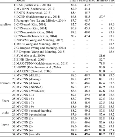
Table 3 compares results on test of MVCNN and its variants with other baselines in the four sen-tence classification tasks. Row 34, “MVCNN (overall)”, shows performance of the best config-uration of MVCNN, optimized on dev. This ver-sion uses five verver-sions of word embeddings, four filter sizes (3, 5, 7, 9), both mutual-learning and pretraining, three convolution layers for Senti140 task and two convolution layers for the other tasks. Overall, our system gets the best results, beating all baselines.
Model Binary Fine-grained Senti140 Subj
baselines
1 RAE (Socher et al., 2011b) 82.4 43.2 – – 2 MV-RNN (Socher et al., 2012) 82.9 44.4 – – 3 RNTN (Socher et al., 2013) 85.4 45.7 – – 4 DCNN (Kalchbrenner et al., 2014) 86.8 48.5 87.4 – 5 Paragraph-Vec (Le and Mikolov, 2014) 87.7 48.7 – – 6 CNN-rand (Kim, 2014) 82.7 45.0 – 89.6 7 CNN-static (Kim, 2014) 86.8 45.5 – 93.0 8 CNN-non-static (Kim, 2014) 87.2 48.0 – 93.4 9 CNN-multichannel (Kim, 2014) 88.1 47.4 – 93.2 10 NBSVM (Wang and Manning, 2012) – – – 93.2 11 MNB (Wang and Manning, 2012) – – – 93.6
12 G-Dropout (Wang and Manning, 2013) – – – 93.4 13 F-Dropout (Wang and Manning, 2013) – – – 93.6
14 SVM (Go et al., 2009) – – 81.6 –
15 BINB (Go et al., 2009) – – 82.7 –
16 MAX-TDNN (Kalchbrenner et al., 2014) – – 78.8 – 17 NBOW (Kalchbrenner et al., 2014) – – 80.9 – 18 MAXENT (Go et al., 2009) – – 83.0 –
versions
19 MVCNN (-HLBL) 88.5 48.7 88.0 93.6
20 MVCNN (-Huang) 89.2 49.2 88.1 93.7
21 MVCNN (-Glove) 88.3 48.6 87.4 93.6
22 MVCNN (-SENNA) 89.3 49.1 87.9 93.4
23 MVCNN (-Word2Vec) 88.4 48.2 87.6 93.4
filters
24 MVCNN (-3) 89.1 49.2 88.0 93.6
25 MVCNN (-5) 88.7 49.0 87.5 93.4
26 MVCNN (-7) 87.8 48.9 87.5 93.1
27 MVCNN (-9) 88.6 49.2 87.8 93.3
tricks 28 MVCNN (-mutual-learning)29 MVCNN (-pretraining) 88.287.6 49.248.9 87.887.6 93.593.2
layers
30 MVCNN (1) 89.0 49.3 86.8 93.8
31 MVCNN (2) 89.4 49.6 87.6 93.9
32 MVCNN (3) 88.6 48.6 88.2 93.1
33 MVCNN (4) 87.9 48.2 88.0 92.4
[image:8.595.101.500.68.544.2]HLBL is removed from row 34, row 28 shows what happens when mutual learning is removed from row 34 etc.
The block “baselines” (1–18) lists some sys-tems representative of previous work on the cor-responding datasets, including the state-of-the-art systems (marked as italic). The block “versions” (19–23) shows the results of our system when one of the embedding versions was not used during training. We want to explore to what extend dif-ferent embedding versions contribute to perfor-mance. The block “filters” (24–27) gives the re-sults when individual filter width is discarded. It also tells us how much a filter with specific size influences. The block “tricks” (28–29) shows the system performance when no mutual-learning or no pretraining is used. The block “layers” (30–33) demonstrates how the system performs when it has different numbers of convolution layers.
From the “layers” block, we can see that our system performs best with two layers of convo-lution in Standard Sentiment Treebank and Sub-jectivity Classification tasks (row 31), but with three layers of convolution in Sentiment140 (row 32). This is probably due to Sentiment140 being a much larger dataset; in such a case deeper neural networks are beneficial.
The block “tricks” demonstrates the effect of mutual-learning and pretraining. Apparently, pre-training has a bigger impact on performance than mutual-learning. We speculate that it is be-cause pretraining can influence more words and all learned word embeddings are tuned on the dataset after pretraining.
The block “filters” indicates the contribution of each filter size. The system benefits from filters of each size. Sizes 5 and 7 are most important for high performance, especially 7 (rows 25 and 26).
In the block “versions”, we see that each em-bedding version is crucial for good performance: performance drops in every single case. Though it is not easy to compare fairly different embedding versions in NLP tasks, especially when those em-beddings were trained on different corpora of dif-ferent sizes using difdif-ferent algorithms, our results are potentially instructive for researchers making decision on which embeddings to use for their own tasks.
6 Conclusion
This work presented MVCNN, a novel CNN ar-chitecture for sentence classification. It com-bines multichannel initialization – diverse ver-sions of pretrained word embeddings are used – and variable-size filters – features of multigranu-lar phrases are extracted with variable-size convo-lution filters. We demonstrated that multichannel initialization and variable-size filters enhance sys-tem performance on sentiment classification and subjectivity classification tasks.
7 Future Work
As pointed out by the reviewers the success of the multichannel approach is likely due to a combina-tion of several quite different effects.
First, there is the effect of the embedding learn-ing algorithm. These algorithms differ in many as-pects, including in sensitivity to word order (e.g., SENNA: yes, word2vec: no), in objective func-tion and in their treatment of ambiguity (explicitly modeled only by Huang et al. (2012).
Second, there is the effect of the corpus. We would expect the size and genre of the corpus to have a big effect even though we did not analyze this effect in this paper.
Third, complementarity of word embeddings is likely to be more useful for some tasks than for others. Sentiment is a good application for com-plementary word embeddings because solving this task requires drawing on heterogeneous sources of information, including syntax, semantics and genre as well as the core polarity of a word. Other tasks like part of speech (POS) tagging may bene-fit less from heterogeneity since the benebene-fit of em-beddings in POS often comes down to making a correct choice between two alternatives – a single embedding version may be sufficient for this.
We plan to pursue these questions in future work.
Acknowledgments
References
Yoshua Bengio, R´ejean Ducharme, Pascal Vincent, and Christian Janvin. 2003. A neural probabilistic lan-guage model. The Journal of Machine Learning Re-search, 3:1137–1155.
William Blacoe and Mirella Lapata. 2012. A com-parison of vector-based representations for semantic composition. InProceedings of the 2012 Joint Con-ference on Empirical Methods in Natural Language Processing and Computational Natural Language Learning, pages 546–556. Association for Compu-tational Linguistics.
Yanqing Chen, Bryan Perozzi, Rami Al-Rfou, and Steven Skiena. 2013. The expressive power of word embeddings. InICML Workshop on Deep Learning for Audio, Speech, and Language Processing. Ronan Collobert and Jason Weston. 2008. A unified
architecture for natural language processing: Deep neural networks with multitask learning. In Pro-ceedings of the 25th international conference on Machine learning, pages 160–167. ACM.
Ronan Collobert, Jason Weston, L´eon Bottou, Michael Karlen, Koray Kavukcuoglu, and Pavel Kuksa. 2011. Natural language processing (almost) from scratch. The Journal of Machine Learning Re-search, 12:2493–2537.
Misha Denil, Alban Demiraj, Nal Kalchbrenner, Phil Blunsom, and Nando de Freitas. 2014. Modelling, visualising and summarising documents with a sin-gle convolutional neural network. arXiv preprint arXiv:1406.3830.
Cıcero Nogueira Dos Santos and Maıra Gatti. 2014. Deep convolutional neural networks for sentiment analysis of short texts. InProceedings of the 25th In-ternational Conference on Computational Linguis-tics.
John Duchi, Elad Hazan, and Yoram Singer. 2011. Adaptive subgradient methods for online learning and stochastic optimization. The Journal of Ma-chine Learning Research, 12:2121–2159.
Alec Go, Richa Bhayani, and Lei Huang. 2009. Twit-ter sentiment classification using distant supervision.
CS224N Project Report, Stanford, pages 1–12. Alex Graves, A-R Mohamed, and Geoffrey Hinton.
2013. Speech recognition with deep recurrent neural networks. InAcoustics, Speech and Signal Process-ing, 2013 IEEE International Conference on, pages 6645–6649. IEEE.
Felix Hill, KyungHyun Cho, Sebastien Jean, Coline Devin, and Yoshua Bengio. 2014. Not all neural embeddings are born equal. In NIPS Workshop on Learning Semantics.
Geoffrey E Hinton, Nitish Srivastava, Alex Krizhevsky, Ilya Sutskever, and Ruslan R Salakhutdinov. 2012.
Improving neural networks by preventing co-adaptation of feature detectors. arXiv preprint arXiv:1207.0580.
Eric H Huang, Richard Socher, Christopher D Man-ning, and Andrew Y Ng. 2012. Improving word representations via global context and multiple word prototypes. InProceedings of the 50th Annual Meet-ing of the Association for Computational LMeet-inguis- Linguis-tics: Long Papers-Volume 1, pages 873–882. Asso-ciation for Computational Linguistics.
Nal Kalchbrenner, Edward Grefenstette, and Phil Blun-som. 2014. A convolutional neural network for modelling sentences. In Proceedings of the 52nd Annual Meeting of the Association for Computa-tional Linguistics. Association for Computational Linguistics.
Yoon Kim. 2014. Convolutional neural networks for sentence classification. InProceedings of the 2014 Conference on Empirical Methods in Natural Lan-guage Processing, October.
Dan Klein and Christopher D Manning. 2003. Ac-curate unlexicalized parsing. InProceedings of the 41st Annual Meeting on Association for Computa-tional Linguistics-Volume 1, pages 423–430. Asso-ciation for Computational Linguistics.
Alex Krizhevsky, Ilya Sutskever, and Geoffrey E Hin-ton. 2012. Imagenet classification with deep con-volutional neural networks. In Advances in neural information processing systems, pages 1097–1105. Quoc V Le and Tomas Mikolov. 2014. Distributed
representations of sentences and documents. In Pro-ceedings of the 31st international conference on Ma-chine learning.
Yong Luo, Jian Tang, Jun Yan, Chao Xu, and Zheng Chen. 2014. Pre-trained multi-view word embed-ding using two-side neural network. In Twenty-Eighth AAAI Conference on Artificial Intelligence. Tomas Mikolov, Martin Karafi´at, Lukas Burget, Jan
Cernock`y, and Sanjeev Khudanpur. 2010. Recur-rent neural network based language model. In IN-TERSPEECH 2010, 11th Annual Conference of the International Speech Communication Association, Makuhari, Chiba, Japan, September 26-30, 2010, pages 1045–1048.
Tomas Mikolov, Kai Chen, Greg Corrado, and Jeffrey Dean. 2013a. Efficient estimation of word represen-tations in vector space. InProceedings of Workshop at ICLR.
Tomas Mikolov, Ilya Sutskever, Kai Chen, Greg S Cor-rado, and Jeff Dean. 2013b. Distributed representa-tions of words and phrases and their compositional-ity. InAdvances in Neural Information Processing Systems, pages 3111–3119.
Andriy Mnih and Geoffrey E Hinton. 2009. A scal-able hierarchical distributed language model. In
Advances in neural information processing systems, pages 1081–1088.
Andriy Mnih and Yee Whye Teh. 2012. A fast and simple algorithm for training neural probabilistic language models. In Proceedings of the 29th In-ternational Conference on Machine Learning, pages 1751–1758.
Bo Pang and Lillian Lee. 2004. A sentimental educa-tion: Sentiment analysis using subjectivity summa-rization based on minimum cuts. InProceedings of the 42nd annual meeting on Association for Compu-tational Linguistics, page 271. Association for Com-putational Linguistics.
Robert Parker, Linguistic Data Consortium, et al. 2009. English gigaword fourth edition. Linguistic Data Consortium.
Jeffrey Pennington, Richard Socher, and Christopher D Manning. 2014. Glove: Global vectors for word representation. Proceedings of the Empiricial Meth-ods in Natural Language Processing, 12.
Richard Socher, Eric H Huang, Jeffrey Pennin, Christo-pher D Manning, and Andrew Y Ng. 2011a. Dy-namic pooling and unfolding recursive autoencoders for paraphrase detection. InAdvances in Neural In-formation Processing Systems, pages 801–809.
Richard Socher, Jeffrey Pennington, Eric H Huang, Andrew Y Ng, and Christopher D Manning. 2011b. Semi-supervised recursive autoencoders for predict-ing sentiment distributions. In Proceedings of the Conference on Empirical Methods in Natural Lan-guage Processing, pages 151–161. Association for Computational Linguistics.
Richard Socher, Brody Huval, Christopher D Manning, and Andrew Y Ng. 2012. Semantic compositional-ity through recursive matrix-vector spaces. In Pro-ceedings of the 2012 Joint Conference on Empiri-cal Methods in Natural Language Processing and Computational Natural Language Learning, pages 1201–1211. Association for Computational Linguis-tics.
Richard Socher, Alex Perelygin, Jean Y Wu, Jason Chuang, Christopher D Manning, Andrew Y Ng, and Christopher Potts. 2013. Recursive deep mod-els for semantic compositionality over a sentiment treebank. InProceedings of the conference on em-pirical methods in natural language processing, vol-ume 1631, page 1642. Citeseer.
Joseph Turian, Lev Ratinov, and Yoshua Bengio. 2010. Word representations: a simple and general method for semi-supervised learning. InProceedings of the 48th annual meeting of the association for compu-tational linguistics, pages 384–394. Association for Computational Linguistics.
Sida Wang and Christopher D Manning. 2012. Base-lines and bigrams: Simple, good sentiment and topic classification. In Proceedings of the 50th Annual Meeting of the Association for Computational Lin-guistics: Short Papers-Volume 2, pages 90–94. As-sociation for Computational Linguistics.
Sida Wang and Christopher Manning. 2013. Fast dropout training. In Proceedings of the 30th In-ternational Conference on Machine Learning, pages 118–126.
Wenpeng Yin and Hinrich Sch¨utze. 2014. An explo-ration of embeddings for generalized phrases. Pro-ceedings of the 52nd annual meeting of the associ-ation for computassoci-ational linguistics, student research workshop, pages 41–47.