An Iteration Method for the Solution of the Eigenvalue Problem of Linear Differential and Integral Operators 1

Journal of Research of the National Bureau of Standards Vol. 45, No. 4, October 1950 Research Paper 2133

An Iteration Method for the Solution of the Eigenvalue

Problem of Linear Differential and Integral Operators

1

By Cornelius Lanczos

The present investigation designs a systematic method for finding the latent roots and the principal axes of a matrix, without reducing the order of the matrix. It is characterized by a wide field of applicability and great accuracy, since the accumulation of rounding errors is avoided, through the process of "minimized iterations". Moreover, the method leads to a well convergent successive approximation procedure by which the solution of integral equations of the Fredholm type and the solution of the eigenvalue problem of linear differ-ential and integral operators may be accomplished.

I. Introduction

The eigenvalue problem of linear operators is of central importance for all vibration problems of physics and engineering. The vibrations of elastic structures, the flutter problems of aerodynamics, the stability problem of electric networks, the atomic and molecular vibrations of particle phys-ics, are all diverse aspects of the same fundamental problem, viz., the principal axis problem of quad-ratic forms.

In view of the central importance of the eigen-value problem for so many fields of pure and applied mathematics, much thought has been de-voted to the designing of efficient methods by which the eigenvalues of a given linear operator may be found. That linear operator may be of the algebraic or of the continuous type; that is, a matrix, a differential operator, or a Fredholm kernel function. Iteration methods play a prom-inent part in these designs, and the literature on the iteration of matrices is very extensive.2 In

the English literature of recent years the works of H. Hotelling [1] 3 and A. C. Aitken [2] deserve

attention. H. Wayland [3] surveys the field in its historical development, up to recent years. W. U. Kincaid [4] obtained additional results by improving the convergence of some of the classical procedures.

1 The preparation of this paper was sponsored in part by the Office of Naval Research.

2 The basic principles of the various iteration methods are exhaustively treated in the well-known book on Elementary matrices by R. A. Frazer, W. J. Duncan, and A. R. Collar (Cambridge University Press, 1938); (MacMillan, New York, N. Y., 1947).

3 Figures in brackets indicate the literature references at the end of this paper.

9 0 4 4 2 8 — 5 0 — — 1

The present investigation, although starting out along classical lines, proceeds nevertheless in a different direction. The advantages of the method here developed 4 can be summarized as

follows:

1. The iterations are used in the most economi-cal fashion, obtaining an arbitrary number of eigenvalues and eigensolutions by one single set of iterations, without reducing the order of the matrix.

2. The rapid accumulation of fatal rounding errors, common to all iteration processes if applied to matrices of high dispersion (large "spread" of the eigenvalues), is effectively counteracted by the method of "minimized iterations".

3. The method is directly translatable into analytical terms, by replacing summation by integration. We then get a rapidly convergent analytical iteration process by which the eigen-values and eigensolutions of linear differential and integral equations may be obtained.

II. The Two Classical Solutions of

Fredholm's Problem

Since Fredholm's fundamental essay on integral equations [5], we can replace the solution of linear differential and integral equations by the solution

4 The literature available to the author showed no evidence that the methods and results of the present investigation have been found before. However, A. M. Ostrowski of the University of Basle and the Institute for Numerical Analysis informed the author that his method parallels the i earlier work of some Russian scientists; the references given by Ostrowski I are: A. Krylov, Izv. Akad. Nauk SSSR 7, 491 to 539 (1931); N. Luzin, Izv. Akad. Nauk SSSR 7, 903 to 958 (1931). On the basis of the reviews of these papers in the Zentralblatt, the author believes that the two methods coincide only in the point of departure. The author has not, however, read these Russian papers.

of a set of simultaneous ordinary linear equations of infinite order. The problem of Fredholm, if formulated in the language of matrices, can be stated as follows: Find a solution of the equation

y—\Ay=b, (1)

where b is a given vector, X a given scalar para-meter, and A a given matrix (whose order event-ually approaches infinity); whereas y is the unknown vector. The problem includes the inversion of a matrix (X= °°) and the problem of the characteristic solutions, also called "eigenso-lutions", (6=0) as special cases.

Two fundamentally different ^classical solutions of this problem are known. The first solution is known as the "Liouville-Neumann expansion" [6]. We consider A as an algebraic operator and obtain formally the following infinite geometric series:

This series converges for sufficiently small values of |X| but diverges beyond a certain |Xl = |Xi|. The solution is obtained by a series of successive "iterations";5 we construct in succession the

following set of vectors:

bo=b

b2=Abx

(3)

and then form the sum:

2

+ . . . . (4)

The merit of this solution is that it requires nothing but a sequence of iterations. The draw-back of the solution is that its convergence is limited to sufficiently small values of X.

The second classical solution is known as the Schmidt series [7]. We assume that the matrix

A is "nondefective" (i. e. that all its elementary

divisors are linear). We furthermore assume that

5 Throughout this paper the term ' 'iteration" refers to the application of the given matrix A to a given vector 6, by forming the product Ab.

we possess all the eigenvalues6 /x^ and eigenvectors Ut of the matrix A, defined by the equations

If A is nonsymmetric, we need also the " adjoint" eigenvectors u<*, defined with the help of the transposed matrix A*:

We now form the scalars b-ut*

(7)

and obtain y in form of the following expansion:

This series offers no convergence difficulties, since it is a finite expansion in the case of matrices of finite order and yields a convergent expansion in the case of the infinite matrices associated with the kernels of linear differential and integral operators.

The drawback of this solution is—apart from the exclusion of defective matrices 7—that it

pre-supposes the complete solution of the eigenvalue problem associated with the matrix A.

III. Solution of the Fredholm Problem by

the S-Expansion

We now develop a new expansion that solves the FredhoJm problem in similar terms as the Liouville-Neumann series but avoids the conver-gence difficulty of that solution.

We first notice that the iterated vectors b0, b\,

b2, . . . cannot be linearly independent of

each other beyond a certain definite bk. All these

vectors find their place within the w-dimensional space of the matrix A, hence not more than n of them can be linearly independent. We thus know in advance that a linear identity of the following form must exist between the successive iterations. \-gmbo=O. (9)

6 We shall use the term "eigenvalue" for the. numbers m defined by (5), whereas the reciprocals of the eigenvalues: \i=l/m shall be called "character, istic numbers".

7 The characteristic solutions of defective matrices (i. e. matrices whose elementary divisors are not throughout linear) do not include the entire /i-dimensional space, since such matrices possess less than n independent principal axes.

We cannot tell in advance what m will be, except for the lower and upper bounds:

l^m^n. (10) How to establish the relation (9) by a systematic algorithm will be shown in section VI. For the time being we assume that the relation (9) is already established. We now define the poly-nomial

G(x)=xm+gixm-l+- • .+gm, (11)

together with the "inverted polynomial" (the coefficients of which follow the opposite sequence):

-+gm\m. (12)

Furthermore, we introduce the partial sums of the latter polynomial:

So =1

(13)

= l+g1\+g2\2

We now refer to a formula which can be proved by straightforward algebra:8

i _

0 • X"-1*—

(14) Let us apply this formula operationally, replacing x by the matrix A, and operating on the vector b0. In view of the definition of the vectors bi.

the relation (9) gives :

G{A) - bo=O,

and thus we obtain:

s

m

(\)

bQ==Sm 1 — A^A and hence: (15) (16) (17) 8 In order to prevent this paper from becoming too lengthy the analytical

details of the present investigation are kept to a minimum, and in a few places the reader is requested to interpolate the missing steps.

If we compare this solution with the earlier solution (4), we notice that the expansion (17) may be conceived as a modified form of the Liou-ville-Neumann series, because it is composed of the same kind of terms, the difference being only that we weight the terms \kbk by the weight factors

-k-i (X)

(18)

instead of taking them all with the uniform weight factor 1. This weighting has the beneficial effect that the series terminates after m terms, instead of going on endlessly. The weight factors Wt are very near to 1 for small X but become more and more important as X increases. The weighting makes the series convergent for all values of X.

The remarkable feature of the expansion (17) is its complete generality. No matter how defective the matrix A may be, and no matter how the vector b0 was chosen, the expansion (17) is always

valid, provided only that we interpret it properly. In particular we have to bear in mind that there will always be m polynomials Sk(k), even though

every Sk(\) may not be of degree Jc, due to the

vanishing or the higher coefficients. For example, it could happen that

so that

and the formula (17) gives:

G(x)=xm, (19)

: +0X-, (20) +0X", (21)

1&W-1. ( 2 2 )

IV. Solution of the Eigenvalue Problem

The Liouville-Neumann series cannot give the solution of the eigenvalue problem, since the ex-pansion becomes divergent as soon as the param-eter X reaches the lowest characteristic number Xi. The Schmidt series cannot give the solution of the eigenvalue problem since it presupposes the knowledge of all the eigenvalues and eigenvectors of the matrix A. On the other hand, the expan-sion (17), which is based purely on iterations and yet remains valid for all X, must contain implicitly the solution of the principal axis problem. In-deed, let us write the right side of (1) in the form

(23) 257

Then the expansion (17) loses its denominator and becomes:

x6m_i. (24)

We can now answer the question whether a solution of the homogeneous equation

y—\Ay=0, (25)

is possible without the identical vanishing of y. The expression (23) shows that b can vanish only under two circumstances; either the vector 6, or the scalar Sm(\) must vanish. Since the former

possibility leads to an identically vanishing y, only the latter possibility is of interest. This gives the following condition for the parameter X.

Sm(X)=0. (26)

The roots of this equation give us the character-istic values X=\i, whereas the solution (24) yields the characteristic solutions, or eigenvalues, or principal axes of the matrix A:

(27)

It is a remarkable fact that although the vector

b0 was chosen entirely freely, the particular linear combination (27) of the iterated vectors has

in-variant significance, except for an undetermined

factor of proportionality that remains free, in view of the linearity of the defining equation (25). That undetermined factor may come out even as zero, i. e., a certain axis may not be represented in the trial vector b0 at all. This explains why the order of the polynomial Sm(\) need not be

neces-sarily equal to n. The trial vector b0 may not give us all the principal axes of A. What we can say with assurance, however, is that all the roots of

Sm(\) are true characteristic values of A, and all the Ui obtained by the formula (24) are true char-acteristic vectors, even if we did not obtain the

complete solution of the eigenvalue problem. The

discrepancy between the order m of the poly-nomial 6(n) and the order n of the characteristic equation

—n . . . aXn

= 0 (28)

will be the subject of the discussion in the next section.

Instead of substituting into the formula (27), we can also obtain the principal axes uf by a numerically simpler process, applying synthetic division. By synthetic division we generate the polynomials:

We then replace xj by bj and obtain:

(30)

The proof follows immediately from the equation (A-m)ui"G(A)'bo=O. (31)

V. The Problem of Missing Axes

Let us assume that we start with an arbitrary "trial vector" b0 and obtain by successive itera-tions the sequence:

bo, b i , b2, . . . , & „ . (32)

Similarly we start with the trial vector b*0 and obtain by iterating with the transposed matrix A* the adjoint sequence:

. . . , 6*. (33)

Let us now form the following set of "basic scalars":

ci+k=brb;=bk'bl (34)

The remarkable fact holds that these scalars depend only on the sum of the two subscripts i and *; e. g.

6*-i6jb+i = 6*-A+i = M*. (35)

This gives a powerful numerical check of the iteration scheme since a discrepancy between the two sides of (35) (beyond the limits of the round-ing errors) would indicate an error in the calcula-tion of bk+1 or b*k+1 if the sequence up to bk and b*k has been checked before.

Let us assume for the sake of the present argu-ment that A is a nondefective matrix, and let us analyze the vector b0 in terms of the eigenvectors*

ut, while b*0 will be analyzed in terms of the adjoint vectors u*:

+rnun, (36)

(37) 258

Then the scalars ct become: with

(38) (39) The problem of obtaining the X from the ci is the problem of "weighted moments", which can be solved as follows: Assuming that none of the

pk vanish and that all the \ are distinct, we establish a linear relation between n+1 consecu-tive ciy of the following form:

y (40)

Then the definition of the ci shows directly that the set (40) demands

where

(41)

(42)

Hence, by solving the recurrent set (40) with the help of a "progressive algorithm", displayed in the next section, we can obtain the coefficients of the characteristic polynomial (42), whose roots give the eigenvalues /x-.

Under the given restricting conditions none of the Hi roots has been lost, and we could actually establish the full characteristic equation (41). It can happen, however, that b0 is orthogonal to some axis u*, and it is equally possible that b*0 is orthogonal to some axis uk. In that case rt and r* drop out of the expansions (36) and (37) and consequently the expansion (38) lacks both

Pi and pk. This means that the scalars cs are unable to provide all the HJ, since ^t and nk are missing. The characteristic equation (41) cannot be fully established under these circumstances.

The deficiency was here caused by an unsuitable choice of the vectors b0 and 6*; it is removable by a better choice of the trial vectors. However, we can have another situation where the deficiency goes deeper and is not removable by any choice of the trial vectors. This happens if the nt roots of the characteristic equation are not all distinct. The expansion (38) shows that two equal roots

\t and X* cannot be separated since they behave

exactly as one single root with a double amplitude. Generally, the weighted moments ct can never show whether or not there are multiple roots, because the multiple roots behave like single roots. Consequently, in the case of multiple eigenvalues the linear relation between the Ci will not be of the

nth but of a lower order. If the number of distinct roots is m, then the relation (40) will appear in the following form:

^ .(43)

Once more we can establish the polynomial

(44)

but this polynomial is now of only mth order and factors into the m root factors

(X — Hi)(x — H2) • • • (X — Mm), (45)

where all the nt are distinct. After obtaining all the roots of the polynomial (44) we can now construct by synthetic division the polynomials:

G(x)

(46)

and replacing xj by bj we obtain the principal axes of both A and A*:

(47)

This gives a partial solution of the principal axis problem, inasmuch as each multiple root con-tributed only one axis. Moreover, we cannot tell from our solution which one of the roots is single and which one multiple, nor can the degree of multiplicity be established. In order to get further information, we have to change our trial vectors and go through the iteration scheme once more. We now substitute into the formulae (47) again and can immediately localize all the single roots by the fact that the vectors % associated with these roots do not change (apart from a propor-tionality factor), whereas the uk belonging to double roots will generally change their direction. 259

A proper linear combination of the newu*k, and the

previous uk establishes the second axis associated with the double eigenvalue jjik; we put

u\=uk u2k = uk+yuk

U2k*=u>k+y*u*k

The factors y and 7* are determined by the con-ditions that the vectors u\ and u% have to be bi-orthogonal to the vectors u\* and uf. In the case of triple roots a third trial is demanded, and so on.

An interesting contrast to this behavior of multiple roots associated with nondefective matri-ces is provided by the behavior of multiple roots associated with defective matrices. A defective eigenvalue is always a multiple eigenvalue, but here the multiplicity is not caused by the collapse of two very near eigenvalues, but by the multi-plicity of the elementary divisor. This comes into evidence in the polynomial G(x) by giving a root factor of higher than first order. Whenever the polynomial G(x) reveals a multiple root, we can tell in advance that the matrix A is defective in these roots, and the multiplicity of the root establishes the degree of deficiency.

I t will be revealing to demonstrate these con-ditions with the help of a matrix that combines all the different types of irregularities that may be encountered in working with arbitrary matrices. Let us analyze the following matrix of sixth order:

1 2 3 0 0 0 0 1 4 0 0 0 0 0 1 0 0 0 0 0 0 2 0 0 0 0 0 0 0 0 L 0 0 0 0 0 0

The eigenvalue 2 is the only regular eigenvalue of this matrix. The matrix is "singular", because the determinant of the coefficients is zero. This, however, is irrelevant from the viewpoint of the eigenvalue problem, since the eigenvalue "zero" is just as good as any other eigenvalue. More important is the fact that the eigenvalue zero is a

double root of the characteristic equation. The

remaining three roots of the characteristic equa-tion are all 1. This 1 is thus a triple root of the characteristic equation; at the same time the matrix has a double deficiency in this root, because the elementary divisor associated with

this root is cubic. The matrix possesses only four independent principal axes.

What will the polynomial G(x) become in the case of this matrix? The regular eigenvalue 2 must give the root factor x—2. The regular eigenvalue 0 has the multiplicity 2 but is reduced to the single eigenvalue 0 and thus contributes the factor x. The deficient eigenvalue 1 has the multiplicity 3 but also double defectiveness. Hence, it must contribute the root factor (x— I)3.

We can thus predict that the polynomial 6{x) will come out as follows.

Let us verify this numerically. As a trial vector we choose

&O= K = 1 , 1 , 1 , 1 , 1 , 1 .

The successive iterations yield the following: bo= 1 1 1 1 1 1 61== 6 b2= 19 63= 40 64= 69 &5=106 66=151 K= 1 b{= 1 K= 1 6 3 = 1 K= 1 6 : = 1 5 9 13 17 21 25 1 3 5 7 9 11 1 1 1 1 1 1 1 8 23 46 77 116 2 4 8 16 32 64 1 2 4 8 16 32 0 0 0 0 0 0 1 0 0 0 0 0 0 0 0 0 0 0 1 0 0 0 0 0 b*6= 1 13 163 64 0 0

We now construct the cx by dotting b0 with the

b* (or b*0 with the bt); we continue by dotting 66

with b*u . . . &e (or b*6 with bu . . . b6). This gives

the following set of 2 ^ + 1 = 13 basic scalars.

Cj = 6, 14, 33, 62, 103, 160, 241, 362, 555, 884,

1477, 2590, 4735.

The application of the progressive algorithm of section VI to these bt yields O(x) in the predicted form. We now obtain by synthetic divisions:

X

2— -VOX X,

Inverting these polynomials we obtain the matrix / 0 - 2 5 - 4 1 0\

1 0 - 1 3 - 3 1 0 1 \ 2 - 7 9 - 5 1 0/

The product of this matrix with the iteration matrix B (omitting the last row bQ) yields three

principal axes Ui) similarly the product of the same matrix with the iteration matrix B* yields the three adjoint axes u*:

= - 8 0 0 0 0 0 u(2)= 0 0 0 2 0 0 u(0)= 0 0 0 0 2 2 u*(l)= 0 0 — 8 0 0 0 u*(2)= 0 0 0 2 0 0 u*(0)= 0 0 0 0 2 2

Since G(x) is of only fifth order, while the order of the characteristic equation is 6, we know that one of the axes is still missing. We cannot de-cide a priori whether the missing axis is caused by the duplicity of the eigenvalue 0, 1, or 2.9

How-ever, a repetition of the iteration with the trial vectors

bo=K=l, 1, 1, 1, 1,0,

causes a change in the row u(0) and u*(0) only. This designates the eigenvalue ^ = 0 as the double root. The process of biorthogonalization finally yields: 10

9 We have in mind the general case and overlook the fact that the

over-simplified nature of the example makes the decision trivial.

w The reader is urged to carry through a similar analysis with the same matrix, but changing the 0, 0 diagonal elements of the rows 5 and 6 to 1, 0, and to 1, 1.

Ui(0)=0 0 0 0 1 1 = 0 0 0 0 1 - 1

ul(0)=0 0 0 0 1 1

u*2(0)=0 0 0 0 1 - 1

VI. The Progressive Algorithm for the

Construction of the Characteristic

Poly-nomial G(x)

The crucial point in our discussions was the establishment of a linear relation between a certain bm and the previous iterated vectors. This relation leads to the characteristic poly-nominal 6(x), whose roots (?(/**) = 0 yield the eigenvalues m. Then by synthetic division we can immediately obtain those particular linear combinations of the iterated vectors bt, which give us the eigenvectors (principal axes) of the matrix A.

We do not know in advance in what relation the order m of the polynomial G(x) will be to the order

n of the matrix A. Accidental deficiencies of the

trial vectors boy b*0, and the presence of multiple eigenvalues in A can diminish m to any value between 1 and n. For this reason we will follow a systematic procedure that generates G(x) gradually, going through all degrees from 1 torn. The procedure comes automatically to a halt when the proper m has been reached.

Our final goal is to solve the recurrent set of equations:

(48)

This is only possible if the determinant of this homogeneous set vanishes:

C\ C\

= 0 . (49)

Before reaching this goal, however, we can cer-tainly solve for any k<Cm the following inhomog-eneous set (the upper k is meant as a superscript):

+ck=0

+ck+1=0

(50)

provided that we put

The freedom of hk in the last equation removes the overdetermination of the set (48). The proper m will be reached as soon as hm turns out to be zero.

Now a recurrent set of equations has certain algebraic properties that are not shared by other linear systems. In particular, there exists a

recurrence relation between the solutions of three

consecutive sets of the type (50). This greatly facilitates the method of solution, through the application of a systematic recurrence scheme that will now be developed.

We consider the system (50) and assume that we possess the solution up to a definite k. Then we will show how this solution may be utilized for the construction of the next solution, which belongs to the order k-\-l.

Our scheme becomes greatly simplified if we consider an additional set of equations that omits the first equation of (50) but adds one more equation at the end :

(51)

Let us now multiply the set (50) by the factor (52)

~ "AT'"A

and add the set (51). We get a new set of equa-tions that can be written down in the form:

(53)

(54)

We now evaluate the scalar

=hk+l (55) which is added to (53) as the last equation.

What we have accomplished is that a proper linear combination of the solutions $ and rft provided us with the next solution i?J+1. But

now exactly the same procedure can be utilized to obtain rji+1 on the basis of vyj and TIJ+1.

For this purpose we multiply the set (51) by (56) and add the set (53), completed by (55) but omitting the first equation.

This gives:

(57)

provided that we put:

(58)

Once more we evaluate the scalar

•> sr/c "T* 1 I I /i r\ (Pv Q A

^ A + 2r7 l " I * * ' ~ TL2 k + 3 'H+2) \OVJ

which is added to (57) as the last equation. This analytical procedure can be translated into an elegant geometrical arrangement that generates the successive solutions iyf and "rjf in successive columns. The resulting algorithm is best ex-plained with the help of a numerical example.

For this purpose we choose the eigenvalue prob-lem of an intentionally over-simplified matrix, since our aim is not to show the power of the

method but the nature of the algorithm, which leads to the establishment of the characteristic equation. The limitation of the method due to the accumulation of rounding errors will be dis-cussed in the next section.

Let the given matrix be:

(

13 5 - 2 3 \ 4 0 - 4 ) 7 3 - 1 3 /

We iterate with the trial vector 60= 1, 0, 0, and

obtain:

1 0 0 13 4 7 28 24 12 208 64 112

We transpose the matrix and iterate with the trial vector 60*=l, 0, 0, obtaining:

1 0 0 13 5 - 2 3 28 —4 —20 208 80 - 3 6 8

We dot the first row and the last row with the opposing matrix and obtain the basic scalars ct as follows:n

1, 13, 28, 208, 448, 3328, 7168.

These numbers are written down in a column, and the scheme displayed below is obtained.

Q' = 1 13 28 208 448 3328 7168 0 1 -13 1 0.5 13 10.84615384 1 1 -141 1.047463173 -13 1 1.5 147. 6923075 1.106382990 -2.15384616 1 2 -163. 4012569 0 -13.617021249 -1.106382987 1 2.5 0 -16.000000004 0. 000000003 1 3 0 0 -16 0 1 (60)

Instead of distinguishing between the rjt and re-solutions we use a uniform procedure but mark the successive columns alternately as "full" and "half columns"; thus we number the successive columns as zero, one-half, one, . . . The scheme has to end at eifull column, and the end is marked by the vanishing of the corresponding "head-number" hi. In our scheme the head-number is zero already at the half-column 2.5, but the scheme cannot end here, and thus we continue to the column 3, whose head-number becomes once more 0, and then the scheme is finished. The last column gives the polynomial G(x), starting with the diagonal term and proceeding upward:

The head-numbers ht are always obtained by dotting the column below with the basic column

d) e. g., at the head of the column 2 we find the

number —163.4042569. This number was ob-tained by the following cumulative multiplication: 448-1+208. (-1.106382987)+28-(-13.617021249). The numbers qt represent the negative ratio of two consecutive hi numbers:

11 Instead of iterating with A and A* n times, we can also iterate with A

alone 2n times. Any of the columns of the iteration matrix can now be chosen as Ci numbers since these columns correspond to a dotting of the iteration matrix with 6j=l, 0, 0, . . ., respectively 0, 1, 0, 0, . . .; 0, 0, 1, 0, 0, . . .; and so on. The transposed matrix is not used here at all. E. C. Bower of the Douglas Aircraft Co. points out to the author that from the machine viewpoint a uniform iteration scheme of 2n iterations is preferable to a divided scheme of n-\-n iterations. The divided scheme has the advan-tage of less accumulation of rounding errors and more powerful checks on the successive iterations. The uniform scheme has the advantage that more than one column is at our disposal. Accidental deficiencies of the 6j vector can thus be eliminated, by repeating the algorithm with a different column. (For this purpose it is of advantage to start with the trial vector 6o=l, 1, 1, . . . 1.) In the case of a symmetric matrix it is evident that after n itera-tions the basic scalars should be formed, instead of continuing with n more iterations.

e- £•> 2i.5=1.106382990 was obtained by the

fol-lowing division:

-(-163.4042569) 147.6923075

The scheme grows as follows. As soon as a certain column d is completed, we evaluate the associated head-number ht) this provides us with

the previous ^-number g[t-H. We now construct

the next column Ci+H by the following operation.

We multiply the column (7*_H by the constant

2*-H a n (i add the column d:

However, the result of this operation is shifted down by one element; e. g. in constructing the column 2.5 the result of the operation

1.10638299-(-2.15384616)+

(-13.617021249) = - 1 6 , is not put in the row where the operation occurred, but shifted down to the next row below.

The unfilled spaces of the scheme are all "zero".

The outstanding feature of this algorithm is that it can never come to premature grief, provided only that the first two c-numbers, c0 and cu are different

from zero. Division by zero cannot occur since the scheme comes to an end anyway as soon as the head-number zero appears in one of the full columns.

Also of interest is the fact that the products of the head-numbers associated with the full columns give us the successive recurrent determinants of the ct; e.g., the determinants

1 and 1 13 1 13 28 208 13 28 13 28 208 448 1 13 ,28 28 208 448 3328 13 28 208 208 448 3328 7168 28 208 448

are given by the successive products

1, l-(—141) = —141, (-141)-(-163.4042569) = 23040, and 23040-0=0, 13 28 28 208 13 28 208 28 208 448 208 448 3328

Similarly the products of the head-numbers of the half-columns give us similar determinants, but omitting c0 from the sequence of c-numbers. In

the example above the determinants 13,

are given by the products:

13, 13-147.6923075 = 1920, 1920-0=0 The purpose of the algorithm (60) was to gener-ate the coefficients of the basic identity that exists between the iterated vectors bt. This identit}"

finds expression in the vanishing of the poly-nomial 6(x):

G(x)=0 (61)

The roots of this algebraic equation give us the eigenvalues of the matrix A. In our example we get the cubic equation

which has the three roots

Mi = 0, /*2=4, / i s = - 4 . (62) These are the eigenvalues of our matrix. In order to obtain the associated eigenvectors, we divide G(x) by the root factors:

Q{x)_, m

x x—4t

This gives, replacing xk by bk:

u(0) = — 16b0

-X + 4:

Consequently, if the matrix

(

- 1 6 0 l \

0 4 l ) 0 - 4 1 /

is multiplied by the matrix of the bt (omitting 63),

(

-16 0 l\ / 1 0 0\ / 12 0 4 1 I I 13 4 7 1=1 80 0 - 4 1/ \28 24 12/ \-24

If the same matrix is multiplied by the matrix of the transposed iterations bt* (omitting 63), we obtain

the three adjoint eigenvectors u]:

(

- 1 6 0 l \ / 1 0 0\ / 0 4 1 I I 13 5 - 2 3 ) = ( 0 - 4 1/ \28 - 4 - 2 0 / \ 12 —4 — 20 - 2 3 1=| 80 16 - 1 1 2 | = - 2 4 - 2 4 72

H

u*(0) \ ti*(4) u * ( - 4 ) / . The solution of the entire eigenvalue problem is thus accomplished.

VII. The Method of Minimized Iterations

In principle, the previous discussions give a com-plete solution of the eigenvalue problem. We have found a systematic algorithm for the generation of the characteristic polynomial G(ii). The roots of this polynomial gave the eigenvalues of the matrix A. Then the process of synthetic division estab-lished the associated eigenvectors. Accidental de-ficiencies were possible but could be eliminated by additional trials.

As a matter of fact, however, the "progressive algorithm" of the last section has its serious limi-tations if large matrices are involved. Let us assume that there is considerable "dispersion" among the eigenvalues, which means that the ratio of the largest to the smallest eigenvalue is fairly large. Then the successive iterations will grossly increase the gap, and after a few iterations the small eigenvalues will be practically drowned out. Let us assume, e. g., that we have a 12 by 12 mat-rix, which requires 12 iterations for the generation of the characteristic equation. The relatively mild ratio of 10:1 as the "spread" of the eigenvalues is after 12 iterations increased to the ratio 1012:l,

which means that we can never get through with the iteration scheme because the rounding errors make all iterations beyond the eighth entirely valueless.

As an actual example, taken from a physical situation, let us consider four eigenvalues, which are distributed as follows:

1, 5, 50, 2000.

Let us assume, furthermore, that we start with a trial vector that contains the four eigenvectors in the ratio of the eigenvalues, i. e., the eigenvalue 2000 dominates with the amplitude 2000, compared with the amplitude of the eigenvalue 1. After one iteration the amplitude ratio is increased to 4-106, after two iterations to 8-109. The later

iterations can give us no new information, since they practically repeat the second iteration, multi-plied every time by the factor 2000. The small eigenvalues 1 and 5 are practically obliterated and cannot be rescued, except by an excessive accuracy that is far beyond the limitations of the customary digital machines.

We will now develop a modification of the cus-tomary iteration technique that dispenses with this difficulty. The modified scheme eliminates the rapid accumulation of rounding errors, which under ordinary circumstances (destroys the value of high order iterations. The new technique pre-vents the large eigenvalues from monopolizing the scene. It protects the small eigenvalues by con-stantly balancing the distribution of amplitudes in the most equitable fashion.

As an illustrative example, let us apply this method of "minimized iterations" to the above-mentioned dispersion problem. If the largest amplitude is normalized to 1, then the initial distribution of amplitudes is characterized as follows:

0.0005, 0.0025, 0.025, 1.

Now, while an ordinary iteration would make this distribution still more extreme, the method of minimized iterations changes the distribution of amplitudes as follows:

0.0205 0.1023 1 —0.0253.

We see that it is now the third eigenvector that gets a large weight factor, whereas the fourth eigenvector is almost completely in the back-ground.

A repetition of the scheme brings about the following new distribution:

0.2184 1 —0.1068 0.0000.

It is now the second eigenvector that gets the strongest emphasis.

The next repetition yields:

1 -0.2181 0.0018 0.0000,

and we see that the weight shifted over to the smallest eigenvalue.

After giving a chance to each eigenvalue, the scheme is exhausted, since we have all the infor-mation we need. Consequently the next mini-mized iteration yields an identical vanishing of the next vector, thus bringing the scheme to its natural conclusion.

In order to expose the principle of minimized iterations, let us first consider the case of symmetric matrices:

A*=A. (63) Moreover, let us agree that the multiplication of a vector b by the matrix A shall be denoted by a prime:

Ab = b'. (64) Now our aim is to establish a linear identity between the iterated vectors. We cannot expect that this identity will come into being right from the beginning. Yet we can approach this identity right from the beginning by choosing that linear combination of the iterated vectors b'o and b0

which makes the amplitude of the new vector as small as possible. Hence, we want to choose as our new vector b\ the following combination:

bi = b'o—aobo, (65)

where a0 is determined by the condition that

(b'o—aobo)2=minimum. (66)

_Kb

0 This gives Notice that 61-60=0, (67) (68)

i.e. the new vector bi is orthogonal to the original vector b0.

We now continue our process. From bx we

proceed to b2 by choosing the linear combination

and once more OLX and

b1-fi0b0f (69)

are determined by the

condition that b\ shall become as small as possible. This gives

«,-f * - * • (70)

U1 00

A good check of the iteration b[ is provided by the condition

Hence, the numerator of /30 has to agree with the

denominator of ai.

The new vector b2 is orthogonal to both b0 and b\.

This scheme can obviously be continued. The most remarkable feature of this successive mini-mization process is, however, that the best linear combination never includes more than three terms. If we form 63, we would think that we should put

But actually, in view of the orthogonality of b2 to

the previous vectors, we get b'2b0 b2bf0

OQ O0

(73)

Hence, every new step of the minimization process requires only two correction terms.

By this process a succession of orthogonal vectors is generated:12

b0, 61, b2, . . ., (74)

until the identity relation becomes exact, which means that

bm=0. (75)

If the matrix A is not symmetric, then we modify our procedure as follows: We operate simultaneously with A and A*.. The operations are the same as before, with the only difference that the dot products are always formed between two opposing vectors. The scheme is indicated as follows:

bo

K

ao—JTJT*^ bl'bQ

bob*o b*ob0

12 The idea of the successive orthogonalization of a set of vectors was prob-ably first employed by O. Szasz, in connection with a determinant theorem of Hadamard; cf. Math, es phys. lapok (in Hungarian) 19, 221 to 227, (1910). The method found later numerous important applications.

b[b*0 bl'b0

2=b'2—a2b2—

o&o

Operationally the prime indicates multiplica-tion by the matrix A. Hence, the succession of

bt vectors represents in fact a successive set oj polynomials. Replacing A by the more familiar

letter xf we have:

b vector system does not come gradually out of gear. However, quite apart from the numerical advan-(76) tages, the biorthogonality of the vectors bt and b) has further appeal because it imitates the behavior

of the principal axes. This is analytically an

eminently valuable fact that makes the transition from the iterated vectors to the principal axes a simple and strongly convergent process.

In order to see the method in actual operation, let us apply it to the simple example of section VI. Here the matrix A is of third order, and thus we have to construct the vectors 60, 61, b2, 63,

and the corresponding adjoint vectors. We ob-tain the following results:

b2=(x—a1)b1—pobo

= (X — am-\) bm-\ -2 = 0

(77)

This gradual generation of the characteristic polynomial G(x) is in complete harmony with the procedure of the "progressive algorithm", dis-cussed in section VI. In fact, the successive

poly-nomials oj the set (77) are identical with the polynomials found in the full columns oj the progres-sive algorithm (60). This explains the existence of

the recurrence relation

Pm+l(x) = (x — an)pn(x) — pn-lPn-l(x), (78)

without additional 7, 5, . . . terms. The existence of such a relation is a characteristic feature of the recurrent set of equations that are at the basis of the entire development.

Although the new scheme goes basically through the same steps as the previously discussed " pro-gressive algorithm", it is in an incomparably stronger position concerning rounding errors. Apart from the fact that the rounding errors do not accumulate, we can effectively counteract their influence by constantly checking the mutual orthogonality of the gradually evolving vectors

bt and 6*. Any lack of orthogonality, caused by rounding errors, can immediately be corrected by the addition of a small correction term.13 By this

procedure the orthogonality of the generated

13 See section IX, eq 90.

bo= 1 0 0 b*0= 1 0 K= 13 5 - 2 3 a0——y-—id 6 1 = b{= 5 - 2 3 &;=-141 - 2 8 - 7 9 _ JL6 7 7 ai - 1 4 1 61' = —141 - 6 9 279 = -11.89361702 62=0, 19.57446808, 4.25531914 b*2=0, -9.53191490, 5.44680854 b'2=0, —17.02127656, 3.40425542 b2=0, 16.34042562, -32.68085142 180.78768715 _ —163.40425746 ft~~ —141 = 1.158895443 &3=0, 0, 0 "2 -163.4042553 = -1.106382981-63=0, 0, 0

The associated polynomials become:

p1(x)=x—13 ) = (x+11.89361702) (x—13) + 141 =x2-1.106382983-13.61702126 = (3+1.106382981) (x*+106382983-13.61702126)-1.158895443(3-13) 267

Comparison with the scheme (60) shows that the coefficients of these very same polynominals appear in the full columns 0, 1, 2, 3, of the pro-gressive algorithm of section VI.

VIII. Solution of the Eigenvalue Problem

by the Method of Minimized Iterations

The biorthogonal property of the vector system bt, b* leads to an explicit solution of the

eigen-value problem, in terms of the vectors bi. Let us first assume that the matrix A is of the nondefec-tive type, and let us analyze the vectors bi in terms of the eigenvectors ut. The method by which the

vectors bt were generated, yields directly the

relation

bi=pi(fi1)u1+pi(fx2)u2+ . . . +Pi(nm)um. (79)

If this relation is dotted with u*k, we obtain, in

view of the mutual orthogonality of the two sets of axes:

bi-u^Piin^Uk-ul (80) Let us now reverse the process and expand the Ui in terms of the bf.

ibm-i. (81)

The dotting by b*k yields:

Let us denote the "norm" of bk by ak:

(83) while the norm of uk will be left arbitrary. Then

the expansion (81) becomes:

G\ 02 O'm-l

(84) This expansion contains the solution of the prin-cipal axis problem. The eigenvectors ut are

gen-erated in terms of the vectors bt, which are the

successive vectors of the process of minimized iterations. The expansion (84) takes the place of the previous "^-expansion" (27), which solved the eigenvector problem in terms of the customary process of iteration.

The adjoint axes are obtained in identical fashion:

C l 0-2

(85)

The expansion (84) remains valid even in the case of defective matrices. The only difference is that the number of principal axes becomes less than n since a multiple root \ih if substituted into

(84) and (85) cannot contribute more than one principal axis.14 However, a defective matrix

ac-tually possesses less than n pairs of principal axes, and the above expansions give the general solution of the problem.

An interesting alternative of the expansion (84) arises if we go back to the original Fredholm problem and request a solution in terms of the minimized vectors bt, rather than the simply

iter-ated vectors of the expansion (17). One method would be to make use of the Schmidt series (8), expressing the ut of that series in terms of the bu

according to the expansion (84). However, the Schmidt series holds for nondefective matrices only, while we know that a solution must exist for any kind of matrices.

Hence, we prefer to proceed in a somewhat different fashion. We expand y directly in terms of the vectors bi'.

(86) We substitute this expansion into the equation (1), replacing b'k by

b'k= (87)

Then we compare coefficients on both sides of the equation. The result can be described as follows: Let us reverse the sequence of the c^-coefficients and let us do the same with the /^-coefficients. Hence, we define

&0 = &m-l

(88)

i* The reader is urged to carry through the process of minimized iterations and evaluation of the principal axes for the defective matrix

/0 1 0\

I 0 0 i j

\0 0 0/

which has only one pair of principal axes; (choose the trial vector in the form 60=&;=l, 1,1).

We now construct the following "reversed" set of polynomials:

Po = 1

V2ix) = (x — x(x) - f t (89)

= G(x)

Then the solution of the Fredholm problem (1) is given by the following expansion:

where we have put

(91) The expansion (90) is completely general and remains valid, no matter how the vector b0 of the right side was given, and how regular or irregular the matrix A may be. The only condition to be satisfied is that the vector b*0—while otherwise chosen arbitrarily—shall be free of accidental deficiencies, i. e., b*0 shall not be orthogonal to some uk if b0 is not simultaneously orthogonal to

<•

The expansion (90) leads once more to a solu-tion of the eigenvector problem, this time obtained with the help of the "reversed" polynomials

Pt(x):

The expansions (92) and (84) actually coincide— except for a factor of proportionality—due to algebraic reasons. /

I

\

12 80 -24 1.10638298 5.10638298 -2.89361702

In order to see a numerical example for this solution of the eigenvalue problem let us return once more to the simple problem of section VI. The minimized bt and b* vectors associated with this matrix were given at the end of section VII. together with the associated polynomials pt(x).

We now construct the reversed polynomials

"pi(x)> For this purpose we tabulate the at and ft:

13 - 1 4 1 -11.89361702 1.158895443 -1.106382981

We reverse the sequence of this tabulation: -1.106382981

-11.89361702 13

'oj>

and construct in succession: (90)

1.58895443 - 1 4 1

Pi (x)=x+1.106382981

.8361702)pi 1.58895443

The last polynomial is identical with pd(x) =

The zeros of this polynomial are: Mi=0, M2=4, j u3= — 4 ;

substituting these values into £>2(M), #I(M)> PO we

obtain the matrix:

12 1.10638298 80 5.10638298 ^—24 —2.89361702

The product of this matrix with the matrix of the

bi vectors gives the three principal axes ut:

0 4 19.57446808 0 \ /

7

M

4.25531914/ ^ f 1 2 80 V — 2 4 24 40 8 12> 40 - 1 6 > k /u(0)

)=U(4)

' V(-4)

\

I

/

269 /

in complete agreement with the previous result of section VI, but now obtained by an entirely different method. If the 6-matrix is replaced by the 6*-matrix, the adjoint axes u*(0), u*(4).

u*(—A) are obtained.

IX. The Lateral Vibrations of a Ear

In order to study the power of the method in connection with a vibration problem of large dispersion, the elastic vibrations of a bar were investigated. The bar was clamped at one end and free at the other. Moreover, the cross section of the bar changes in the middle, as shown in figure 1.

FIGURE 1. Elastic bar, clamped at one end, free at the other; the moment of inertia makes a jump in the middle in the ratio 1:2.

The change of the cross section was such that the moment of inertia jumped from the value 1 to 2. The differential equation that describes the vibra-tions of such a bar is the following fourth-order equation:

( 9 3 )

with the boundary conditions:

2/(0) = o y"(D=o

y'(0)=0 y'"(D=0 and

(94)

(95) The differential operator d/dx was replaced by the difference operator A/Ax, with A^ = l. The length of the bar was chosen as 1=13, thus leading to a 12 by 12 matrix; (since y(0)=y(l)=0).

The first step was the inversion of the matrix. This was easily accomplished, since a matrix that is composed of a narrow band around the diagonal can be inverted with little labor. The eigenvalues

Hi of the inverted matrix are the reciprocals of the

original X*:

//*

= f-

(96)

The general theory has shown that the iteration scheme applied to an arbitrary matrix automati-cally yields a biorthogonal set of vectors bt and b*; they can be conceived as the building blocks from which the entire set of principal axes may be gener-ated. In the present problem dissipative forces are absent, which makes the matrix A symmetric and the problem self-adjoint. Hence,

bt=b:, (97)

and we get through with a single set of iterations. Now the general procedure would demand that we go through 12 minimized iterations before the stage b12=0 is attained. However, the study of a

system with high dispersion has shown that in such a system the method of minimized iterations practically separates the various vibrational modes, starting with the highest eigenvalue and descending systematically to the lower eigenvalues, provided that we employ a trial vector b0 which weights the eigenvectors approximately accord-ing to the associated eigenvalues. In the present problem the trial vector 1, 0, 0 . . ., was not used directly but iterated with the matrix A, and then iterated again. The thus obtained vector b"0 was employed as the b0 of the minimized iteration scheme.

The strong grading of the successive eigen-vectors has the consequence that in k minimized iterations essentially only the highest k vibrational modes will come into evidence. This is of eminent practical value, since it allows us to dispense with the calculation of the very low eigenvalues (i. e., very high frequencies since we speak of the eigen-values of the inverted matrix), which are often of little physical interest, and also of little mathe-matical interest, in view of the fact that the replacing of the d operator by the A operator be-comes in the realm of high frequencies more and more damaging.

Whether the isolation actually takes place or not can be tested with the help of the pt(x)

poly-nomials, which accompany the iteration scheme. The order of these polynomials constantly increases by 1. The correct eigenvalues of the matrix A are obtained by evaluating the zeros of the last polynomial pm(x)=0. What actually happens, however, is that the zeros of the polynomials

Pi(x) do not change much from the beginning.

If the dispersion is strong, then each new poly-nomial basically adds one more root but corrects the higher roots by only small amounts. It is

thus well possible that the series of largest roots in which we are primarily interested is practically established with sufficient accuracy after a few iterations. Then we can stop, since the later iterations will change the obtained values by negli-gible amounts. The same can be said about the vibrational modes associated with these roots.

This consideration suggests the following succes-sive procedure for the approximate determination of the eigenvalues and eigenvectors (vibrational modes) of a matrix. As the minimization scheme proceeds and we constantly obtain newer and newer polynomials pt(x), we handle the last poly-nominal obtained as if it were the final polynomial

pm(x). We evaluate the roots of this polynomial and compare them with the previous roots. Those roots that change by negligible amounts are already in their final form.

A similar procedure holds for the evaluation of the eigenvectors u{. Here the biorthogonality of

the vectors bt and 6* —which is reduced to simple orthogonality in the case of a symmetric matrix— is of very great help. Let us assume that the length of the vectors bt is normalized to 1, by replacing bt by billet. Then the expansions (84) and (85) show that the following matrix must be an orthogonal—although in the diagonal terms not normalized—matrix:

P2M

Pm-l (Mm) (98)

The dot-product of any two rows of this matrix must come out as zero—thus providing us with a powerful check on the construction of the pt poly-nomials and the correctness of the roots /**, which are the roots of the equation ^m(M)=0.15 In the

case of strong dispersion, the transformation matrix (98) is essentially reduced to the diagonal terms and one term to the right and to the left of the diagonal; i. e., the eigenvector uk is essentially a linear combination of three 6-vectors only, viz., bk-2, &Ar—1. a n d bk.

These general conditions are well demonstrated by the tabulation of the final results of the above-mentioned bar problem. The minimized itera-tions were carried through up to m—6. On the basis of these iterations the first six eigenvalues and the first five vibrational modes of the clamped-free bar were evaluated. The iterations were con-stantly watched for orthogonality. After obtain-ing a certain bt, this bt was immediately dotted with all the previous bj. If a certain dot-product

bt - bj came out as noticeably different from zero, the correction term

€ij= j-y- bj, (99)

was added to bf, thus compensating for the

in-fluence of rounding errors. By this procedure the 10 significant figure accuracy of the calculations was constantly maintained.16

The roots of the successive polynomials pt{x) are

tabulated as follows: Ml 2256.926071 .943939 .943939 . 943939 .943939 .943939 M4 1.513923859 .582259337 . 5829955952 M2 48.1610705 . 2037755 . 2037825 . 2037825 . 2037825 M5 0. 546327303 . 591117817 M3 5.272311428 .355958260 . 356269794 .356269980 M6 6. 2498132719

" Due to reasons of algebra, the orthogonality of the matrix (98) holds not only for the final m but for any value of m.

16 In a control experiment that imitated the conditions of the vibrating bar but with a more regular matrix, the results were analytically predictable and the computational results open to an exact check. This example vividly demonstrated the astonishing degree of noninterference of orthogonal vectors. The spread of the eigenvalues was 1 : 3200. The trial vector fro strongly over-emphasized the largest eigenvalue, containing the lowest and the highest eigenvectors with an amplitude ratio of 1:108; (this means that if the vector of the smallest eigenvalue were drawn with the length of 1 in., the vector of the largest eigenvalue, perpendicular to the previous one, would span the distance from Los Angeles to Chicago). The slightest inclination between the two vectors would fatally injure the chances of the smallest eigenvalue. When the entire computation scheme was finished, the analytically required eigenvalues were computed and the comparison made. The entire set of

eigenvalues, including the last, agreed with a maximum error of 2 units in the ninth significant figure, thus demonstrating that the method is completely

free of the cumulation of rounding errors. The author is indebted to Miss Fannie M. Gordon, of the National Bureau of Standards, for the eminently careful and skilled performance of the computing operations.

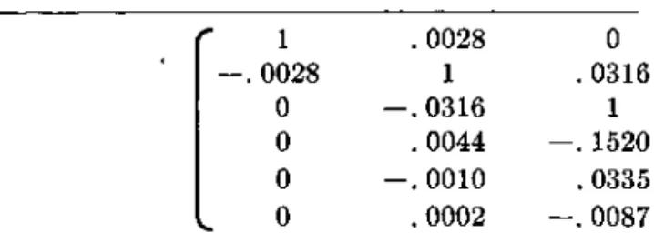
The successive orthogonal transformation ma-trices (98) show likewise strong convergence. We tabulate here only the last computed trans-formation matrix (rounded off to four decimal places), which expresses the first six eigenvectors

U\, . . ., u& in terms of the first six nor-malized bi/-\lcri vectors, making use of the roots of p6(u)=0. The diagonal elements are

nor-malized to 1: 1 0028 0 0 0 0 .0028 1 -.0316 .0044 -.0010 .0002 0 .0316 1 -. 1520 .0335 -.0087 0 .0004 . 1497 1 -. 2793 .0779 0 0 .0081 .2693 1 -.3816 0 0 0 . 0249 .4033 1

We notice how quickly the elements fall off to zero as soon as we are beyond one element to the right and one to the left of the main diagonal. The orthogonal reference system of the bt and the orthogonal reference system of the ut are thus in close vicinity of each other.

The obtained five vibrational modes ux . . ., u5

(u6 being omitted since the lack of the neigh-bour on the right side of the diagonal makes the approximation unreliable) are plotted graphically in figure 2.

- 5

0 2 4 6 8 10 12 14

FIGURE 2. The first five lateral vibrational modes of the elastic bar, shown in figure 1.

Mi=2256.94; ju2=48.20; ju3=5.36; ^4=1.58; M S = 0 . 5 9

X. The Eigenvalue Problem of Linear

In-tegral Operators

The methods and results of the past sections can now be applied to the realm of continuous operators. The kernel of an integral equation can be conceived as a matrix of infinite order, which may be approximated to any degree of accuracy by a matrix of high but finite order. One method of treating an integral equation is to replace it by an ordinary matrix equation of

sufficiently high order. This procedure is, from the numerical standpoint, frequently the most satisfactory one. However, we can design meth-ods for the solution of integral equations that obtain the solution by purely analytical tools, on the basis of an infinite convergent expansion, such as the Schmidt series, for example. The method we are going to discuss belongs to the latter type. We will find an expansion that is based on the same kind of iterative integrations as the Liouville-Neumann series, but avoiding the convergence difficulties of that expansion. The expansion we are going to develop converges

under all circumstances and gives the solution of

any Fredholm type of integral equation, no matter how defective the kernel of that integral equation may be.17

Let us first go back to our earlier method of solving the Fredholm problem. The solution was obtained in form of the S-expansion (17). The difficulty with this solution is that it is based on the linear identity that can be established between the iterated vectors bt. That identity

is generally of the order n; if n grows to infinity, we have to obtain an identity of infinite order before our solution can be constructed. That, however, cannot be done without the proper adjustments.

The later attempt, based on the method of minimized iterations, employs more adequate principles. We have seen that to any matrix,

A, a biorthogonal set of vectors bt and b] can

be constructed by successive minimizations. The set is uniquely determined as soon as the first trial vectors b0 and b*0 are given. In the case A

of the inhomogeneous equation (1) the right side

b may be chosen as the trial vector b0, while b*Q is still arbitrary.

i7 The Volterra type of integral equations, which have no eigenvalues and eigensolutions, are thus included in our general considerations.

The construction of these two sets of vectors is quite independent of the order n of the matrix. If the matrix becomes an integral operator, the

bt and b] vectors are transformed into a

bior-thogonal set of functions:

(100) <t>*o(x),

which are generally present in infinite number. The process of minimized iterations assigns to

any integral operator such a set, after <j>0(x) and

<l>*o(x) have been chosen.

Another important feature of the process of minimized iterations was the appearance of a successive set of polynomials Pi(y), tied together by the recurrence relation

pi+1(») = (v — (101)

This is again entirely independent of the order n of the matrix A and remains true even if the matrix A is replaced by a Fredholm kernel K(x,£). We can now proceed as follows. We stop at an arbitrary pm(x) and form the reversed set of polynomials pi(/x), defined by the process (88). Then we construct the expansion:

(102) This gives a successive approximation process that converges well to the solution of the Fredholm integral equation y(x)—\Ky(x)=<t>Q(x). In other words: (x) = \imym(x). (103) (104) By the same token we can obtain all the eigen-values and eigensolutions of the kernel K(x}£),

if such solutions exist. For this purpose we obtain the roots /** of the polynomial pm(ix) by

solving the algebraic equation

2>m(/0=0. (105) The exact eigenvalues nt of the integral operator

K(x£) are obtained by the limit process:

(106)

where the largest root is called nlf and the sub-sequent roots are arranged according to their absolute values. The corresponding eigenfunc-tions are given by the following infinite expansion:

M«(aO = lim

(107) where yn is the ith root of the polynomial jpm(/x).18

As a trial function #0(#) we may choose for

example

o—const. = 1. (108) However, the convergence is greatly speeded up if we first apply the operator K to this function, and possibly iterate even once more. In other words, we should choose <I>O—K-1, or even <J>Q=--K2-1 as the basic trial function of the expansion (107).

We consider two particularly interesting ex-amples that are well able to illustrate the nature of the successive approximation process here dis-cussed.

(A) The vibrating membrane. In the problem of the vibrating membrane we encounter the fol-lowing self-adjoint differential operator:

This leads to the eigenvalue problem

dO9)

), (HO)

with the boundary condition

2/(l)=0. (HI) The solution of the differential equation (110) is y = J0( 2 V t a ) , (112)

where Jo(x) is the Bessel-function of the order zero. The boundary condition (111) requires that X shall be chosen as follows:

(113) where £* are the zeros of JQ(X).

i8 This expansion is not of the nature of the Neumann series, because the coefficients of the expansion are not rigid but constantly changing with the number m of approximating terms.

Now the Green's function of the differential equation (110) changes the differential operator (109) to the inverse operator, which is an integral operator of the nature of a symmetric Fredholm kernel function K(x, £). Our problem is to obtain the eigenvalues and eigenfunctions of this kernel. If we start out with the function 0o(#) = l, the operation K<j)Q gives

l-x,

and repeating the operation we obtain

and so on. The successive iterations will be

polynomials in x. Now the minimized iterations

are merely some linear combinations of the ordi-nary iterations. Hence the orthogonal sequence

<t>i{x) will become a sequence of polynomials of

constantly increasing order, starting with the constant <£0=l- This singles out the <t>k{x) as the

Legendre polynomials Pk(x), but normalized to

the range 0 to 1, instead of the customary range — 1 to + 1 . The renormalization of the range transforms the polynomials Pk(x) into Jacobi polynomials Gk(p, q; x), with p=g=l [8], which

again are special cases of the Gaussian hypergeo-metric series F(a, (3, y; x), in the sense of F(k-\-\,

—k, 1; x); hence, we get:

(114)

The associated polynomials pt(x) can be obtained

on the basis of the relation:

This gives: Pu = 1 Vl(x)=2x-1 (116) p2(x)=24x2- l&c+l #3(z)=720r3-600;z2+72;z-l

In order to obtain the general recurrence relation for these polynomials it is preferable to follow the example of the algorithm (60) and introduce the "half-columns" in addition to the full columns. Hence, we define a second set of polynomials qk(x)

and set up the following recurrence relations: (117)

pn (x) =nxqn_1 (x) —pn-i (x)

qn(x)=2(2n+ l)pn(x) -qn-i{x)

We thus obtain, starting with po=l and qo=2,

and using successive recursions: 2o=2 p1(x)=2x-l p2(x)=24:X2~lSx+l ps(x)=720x3 -600z2+72z-l 8 q2(x)=24:0x2—l92x + 18 1200x-32 (118) The zeros of the pm(x) polynomials converge to

the eigenvalues of our problem, but the conver-gence is somewhat slow since the original function 0o=l does not satisfy the boundary conditions and thus does not suppress sufficiently the eigen-functions of high order. The zeros of the qt poly-nomials give quicker convergence. They are tabulated as follows, going up to q5(x):

(119)

The last row contains the correct values of the eigenvalues, computed on the basis of (113):

M<=p- (120) We notice the excellent convergence of the scheme. The question of the eigenfunctions of our prob-lem will not be discussed here.

(B) The vibrating string. Even modes. Another interesting example is provided by the vibrating string. The differential operator here is

Ml 0. 6667 . 69155 . 69166016 . 6916602716 . 6916602760 . 6916602761 M2 0.1084 .130242 .1312564 .13127115 .13127123 M3 . 035241 .051130 .0532914 . 0534138 .014842 .025582 . 028769 M5 \~00729 ' . 01794 274

d2

~W

2

'

with the boundary conditions

sK±i)=o.

The solution of the differential equation

d2

(121)

(122)

(123) under the given boundary conditions is:

yi=cos (2i+l) -^ x (evenmodes). (124)

^ = s i n JTX (odd modes). (125) This gives the eigenvalues:

(

2i-\-l V

—s— 7r j (even modes), (126)

X,= (JTT)2 (odd modes). (127)

and

If we start with the trial function 0O=1, we will

get all the "even vibrational modes of the string, while cl>o=x will give all the odd vibrational modes. We first choose the previous alternative.

Successive iterations give

^2__1 x4_x^ 5_ = 24 4i~ 2 4 .

(128)

and we notice that the minimized iterations will now become a sequence of even polynomials. The transformation x2 = £ shows that these polynomials

are again Jacobi polynomials Gk(p, q; a:2), but now

p=q=±i and we obtain the hypergeometric

func-tions F(Jc+\,-k, i ; z2) :

02(x)—3—30a:2+35x4

03 (x) = 5 — 105x2+315x4—231x6

(129)

Once more we can establish the associated polynomials Pi(x), and the recurrence relation by which they can be generated. In the present case the recurrence relations come out as follows:

pn(x) = (An—

starting with po=l,

(130) This yields

2o=l (131)

The successive zeros of the qt(x) polynomials,

up to qs(x), are tabulated as follows:

Mi 0.40000 . 405059 . 405284733 . 4052847346 . 4052847346 . 4052847346 M2 0.02351 . 044856 . 04503010 . 0450316322 . 0450316371 M3 0.011397 . 015722 .016192 . 016211 M4 0.00455 .00752 . 00827 M5 0.00216 .00500

The last row contains the correct eigenvalues, calculated from the formula:

(132) The convergence is again very conspicuous.

(C) The vibrating string. Odd modes. In the case of the odd modes of the vibrating string, the orthogonal functions of the minimized itera-tions are again related to the Jacobi polynomials

Gk(p,q;x), but now with £>=g=3/2. Expressedin terms of the hypergeometric series we now get the polynomials of odd orders

| , - i f c , | ;